Indicators and trends for EU urban areas - JRC Publications ...

Indicators and trends for EU urban
areas
 Data and methods in the
 LUISA platform in support to
 EU Urban and Regional Policy

 Ricardo Ribeiro Barranco, Jean-Philippe Aurambout, Filipe
 Batista e Silva, Mario Marin Herrera, Christiaan Jacobs,
 Carlo Lavalle

 2014

 Report EUR 27006 EN

European Commission

Joint Research Centre

Institute for Environment and Sustainability

Contact information

Carlo Lavalle

Address: Joint Research Centre, Via Enrico Fermi 2749, TP 270, 21027 Ispra (VA), Italy)

E-mail: carlo.lavalle@jrc.ec.europa.eu

39 0332 78 5231

https://ec.europa.eu/jrc

Legal Notice

This publication is a Science and Policy Report by the Joint Research Centre, the European Commission’s in-house science
service. It aims to provide evidence-based scientific support to the European policy-making process. The scientific output
expressed does not imply a policy position of the European Commission. Neither the European Commission nor any person
acting on behalf of the Commission is responsible for the use which might be made of this publication.

All images © European Union 2015,

JRC93888

EUR 27006 EN

ISBN 978-92-79-44673-3 (PDF)

ISSN 1831-9424 (online)

doi: 10.2788/627179

Luxembourg: Publications Office of the European Union, 2015

© European Union, 2015

Reproduction is authorised provided the source is acknowledged

Abstract

This report covers two elements of work that are part of a wider framework aiming to support the evaluation and
sustainability assessment of territorial cohesion and urban development in Europe.

The first element concerns the creation of an urban historical time series, using two European-wide geo-databases
(MOLAND and Urban Atlas). The second element is a new methodological approach to calculate and quantify urban sprawl
based upon the definition of the Weighted Urban Proliferation Index (WUP). The two elements contribute to the further
development of the structured database and methodological framework of Land Use-based Sustainability Assessment
(LUISA) platform, which is developed by the JRC to contribute to the territorial Impact Assessment of EU policies in an
integrated manner with coherent and consistent assumptions.

The work on MOLAND, Urban Atlas and WUP that are presented in this report contribute to the preparation of the EC/UN-
Habitat report “The State of European Cities 2016”.

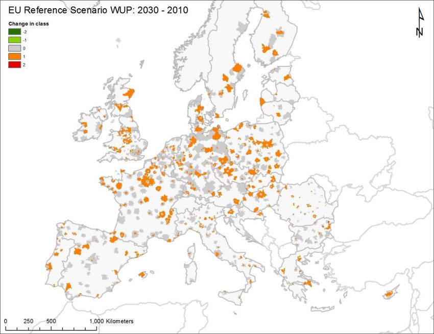
Table of Contents .......................................................................................................................................... 1
1. Introduction .......................................................................................................................................... 3
2. The MOLAND and the Urban Atlas geo-databases ............................................................................... 4
 2.1. Revisiting the MOLAND Data set ....................................................................................................... 5
 2.2. Urban Atlas: A systematic way of mapping ....................................................................................... 7
 2.3. Bottom-line: the compromise against the dream of the cartographer ............................................. 8
3. Integrating the MOLAND and the Urban Atlas geo-databases ............................................................. 8
4. Urban expansion in European cities. Exploring the MOLAND-UATL time series .................................... 15
5. Discussion and conclusions regarding the generation of urban historical time series data .................. 21
6. Weighted Urban Proliferation Index ....................................................................................................... 22
 6.1 Methods ............................................................................................................................................ 23
 6.2 Preliminary results and interpretation ............................................................................................. 25
7. Conclusions and future steps .................................................................................................................. 28
8. References .............................................................................................................................................. 29

 1

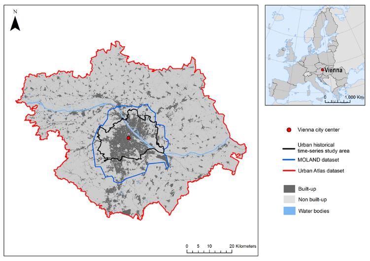
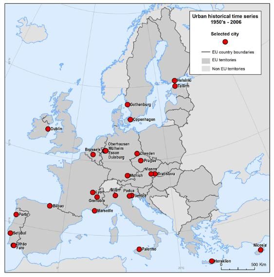
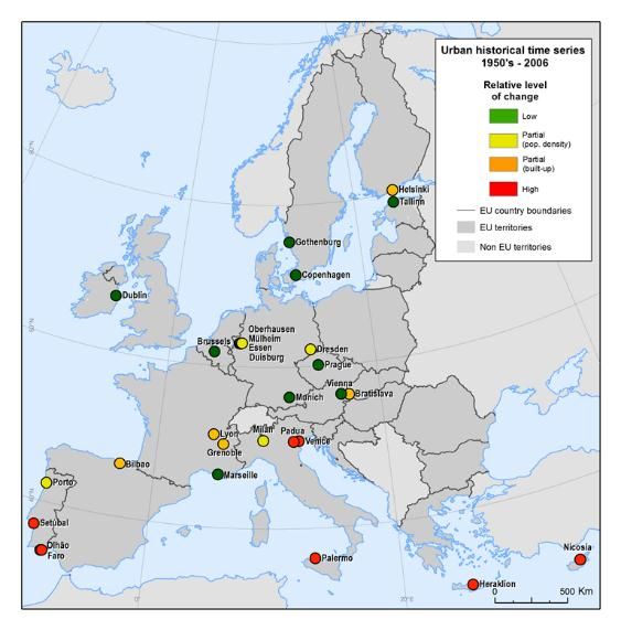
Figures
Figure 1. Work flow to combine MOLAND and the Urban Atlas. ................................................................. 9
Figure 2. Selection of cities available in both MOLAND and the Urban Atlas. ........................................... 10
Figure 3. Vienna: Urban Atlas mapping extent (in red), MOLAND mapping extent (in blue), and urban
cluster (black line) ....................................................................................................................................... 11
Figure 4. Example of thematic and spatial harmonization between the MOLAND and UA data sets for a
specific site in Vienna, Austria. ................................................................................................................... 13
Figure 5. Structure of the final geo-database. ............................................................................................ 14
Figure 6. Urban expansion in Vienna, Prague, Palermo, and Helsinki between 1950 and 2006. ............... 16
Figure 7. Share of different land use/cover types for Vienna, Prague, Palermo, and Helsinki between 1950
and 2006. .................................................................................................................................................... 17
Figure 8. Population and built-up growth between 1950 and 2006........................................................... 19
Figure 9. Increase in built-up areas and decrease in population density between 1950 and 2006............ 20
Figure 10. Typology of cities according to the scatter-plot classification................................................... 20
Figure 11. Illustration of the cell distance calculation procedure. .............................................................. 24
Figure 12: Pixel WUP for 2010 reference scenario for W. Vienna, in Austria. ............................................ 25
Figure 13: WUP aggregated for large urban zone of changes in WUP between 2010 and 2030 under a
reference policy scenario. ........................................................................................................................... 27
Figure 14: WUP aggregated at country level and representing changes in WUP between 2010 and 2030
under a reference policy scenario. .............................................................................................................. 28

Tables
Table 1. Urban Areas mapped by the MOLAND project............................................................................... 5
Table 2. Main characteristics of the MOLAND and the Urban Atlas land use/cover datasets. .................... 8
Table 3. Land use classification used in the combined geo-database. ....................................................... 12
Table 4. Population, built-up area and population density in 1950 and 2006 for the cities mapped in the
combined geo-database. ............................................................................................................................ 18

 2

1. Introduction
Due to their importance and role as primary ‘human ecosystems’, cities have always attracted great
attention from researchers from both social and earth sciences. Cities played a key role in human and
social development over History, and continue to do so, as they draw vast numbers of people into a
safe, organized and culturally-rich environment, enabling creative interaction, developing critical mass
and generating economies of scale (Bettencourt, Lobo, Helbing, Kuhnert, and West. 2007; Bettencourt,
2013; Batty, 2013).

Although cities have been studied from almost every perspective throughout the centuries, the interest
on their impact on the environment is more recent. It has been observed that urbanization processes
are drivers of economic growth (Bloom, Canning, and Fink, 2008), but extreme urbanization rates can
also generate crowding (Bettencourt, 2013), environmental degradation, and other impediments to
well-being and productivity (Bai, Chen, and Shi, 2012).

European Union (EU) cities continue to hold an ever increasing share of EU’s population and expand
their physical boundaries. Recent assessments show that land taken for built-up areas increases more
rapidly than the population in many European countries (OECD, 2012). Many underlying factors have
been attributed to the different pace of growth of population and urban extent. Wide access to
automobiles and mass transportation allows people to live away from where they work, which may lead
to more widespread, dispersed urban areas (Ewing, 1997; Burchell et al., 1998)—a trend already noted
by Webber (1964). In addition, increases in GDP per capita and the fragmentation of households have
been leading to higher per capita demand for residential space.

Despite the important economic, social, and cultural role of cities, their ever increasing size has been
raising concerns over environmental degradation, such as increased pollution, disruption of ecosystems,
and destruction of soils and cultivable areas that otherwise could be used for purposes such as
agriculture (Seto, Woodcock, Song, Huang, Lu, and Kaufmann, 2002; Seto, Guneralp, and Hutyra, 2012).
The expansion of built-up areas, in effect, constitutes an important change in the local environmental
conditions and landscape, and these changes are often extremely costly to reverse (Seto, Fragkias,
Guneralp, and Reilly. 2011). Moreover, recent forecasts of urban expansion reveal that globally, urban
extent in 2030 may be as much as three times that in 2000 if current trends in population density
continue (Seto et al., 2012).

This report covers two elements of work that are part of a wider framework aiming to support the
evaluation and sustainability assessment of territorial cohesion and urban development in Europe.

The first element concerns the creation of an urban historical time series, using two European-wide geo-
databases (MOLAND and Urban Atlas, Barranco et al, 2014). The second element is a new
methodological approach to calculate and quantify urban sprawl based upon the definition of the
Weighted Urban Proliferation Index (WUP)..The two elements contribute to the further development of
the structured database and methodological framework of Land Use-based Sustainability Assessment
(LUISA) platform, which is developed by the JRC to contribute to the territorial Impact Assessment of EU

 3

policies in an integrated manner with coherent and consistent assumptions. The creation of the urban
historical time series will be explained in sections 2 to 5, elaborating on the used databases in section 2,
the method to integrate those databases in section 3, descriptive results of the historical time series in
section 4 and some concluding thoughts in section 5. An explanation of the WUP indicator and an
exploration of WUP values in the just presented historical time series is given in section 6. Some
concluding remarks on the value of the presented work are finally given in section 7.

Last but not least, the work on MOLAND, Urban Atlas and WUP that are presented in this report
contribute to the preparation of the EC/UN-Habitat report “The State of European Cities 2016”.

 2. The MOLAND and the Urban Atlas geo-databases
Long aware of the issues urban areas face, the European Commission has been interested in promoting
more sustainable cities (CEC, 1990). One important approach includes promoting the efficient use of
land, thus avoiding costs related to uncontrolled sealing of soil (EC, 2011) and sprawling cities. Before
addressing the sustainability issues of cities, it is important to acquire knowledge about and understand
the nature of the challenge (Batista e Silva and Marques 2010). Several actions have therefore been
promoted to assess the state of European cities. The project, Monitoring Urban Dynamics and the
follow-up project, Monitoring Land Use/Cover Dynamics (MOLAND), are two well-known initiatives
spearheaded by the European Commission since 1998. These projects, hereinafter denoted simply as
MOLAND, are intended to monitor the development of European urban areas. The MOLAND approach
was in fact threefold: mapping the past land use changes in cities, understanding the observed urban
dynamics, and forecasting future urban land use changes (Lavalle, Niederhuber, McCormick, and
Demicheli, 2000; EEA, 2002). As a result of the first mapping stage, land use and land use changes were
mapped for a sample of more than 30 European cities and regions covering the period of the 1950s to
the late 1990s. This mapping effort yielded a valuable digital geo-database that has been used in
numerous assessments (McCormick, Lavalle, Niederhuber, and Demicheli, 2000; Demicheli et al., 2001;
Barredo, Kasanko, McCormick, and Lavalle, 2003; Kasanko, Barredo, Lavalle, McCormick, Demicheli,
Sagris, and Brezger, 2006). Late in the decade 2001–2010, the European Commission, through the
program, Global Monitoring for Environment and Security (GMES), began funding the Urban Atlas (UA),
which consists of a series of detailed land use maps for 2006 (± one year), covering more than 300 large
urban zones across the European Union.

Whereas both geo-databases are compatible with the CORINE Land Cover nomenclature, the MOLAND
and the UA geo-databases are not directly nor easily interchangeable because of various differences in
cartographic specifications. In this paper, we aim to revamp the MOLAND database from the digital
archives and integrate the newly available data from the UA, thus adding an extra time step to the
MOLAND time series. As it has gained form, integration of the two geo-databases has revealed some
technical challenges, but it also turned out to be a promising effort that would allow the reuse and
expansion of a valuable historical time series of urban land use/cover for a representative sample of
nearly 30 European urban areas.

 4

The following sections describes in more detail the MOLAND and Urban Atlas geo-databases. In the next
section, we define a methodological workflow to combine both data sets into a single, consistent, and
extended time series of urban land use for the set of selected cities. In the section following, some basic
results and indicators yielded from the newly combined geo-database are presented, with a focus on
urban growth and urban land use intensity measures and maps. The concluding section discusses both
the potentialities and limitations of the integrated geo-database and points toward future work.

2.1. Revisiting the MOLAND Data set

The MOLAND geo-database consists of a time series of land use maps, transport network data, and
statistical data for a set of European cities and regions. In this report we primarily focus on the land use
data for each city or region.

MOLAND land use data was built upon coordination of information on the environment (CORINE) Land
Cover (CLC) map specifications (EEA, 2002; Kasanko et al., 2006). CLC is an ongoing mapping project that
has mapped the pan-European land use for circa 1990, 2000, and 2006. The nominal spatial scale of CLC
is 1:100,000, and it has a minimum mapping unit of 25 hectares and a thematic resolution of forty-four
land use/cover classes organized in a three-tier hierarchical structure. MOLAND intended to monitor the
land use/cover classes at city level, and so it required significant additional detail. It was therefore
designed with a nominal scale of 1:25,000, a minimum mapping unit of 1 hectare for artificial land
covers, and 3 hectares for non-artificial land covers. The land use/cover nomenclature was built upon
that of CLC. Two additional hierarchical levels were added to those of CLC, reaching nearly 100 land use
classes, thus substantially increasing the thematic detail of the original CLC land use/cover
nomenclature. The selection of the cities was determined to guarantee a satisfactory representativeness
of European mid- to large-sized cities from all corners of Europe. In total, approximately 30 urban areas
were mapped. In most cases, the mapped areas corresponded to individual cities, but some transport
corridors and other more extended urban areas were included as well (Table 1).

To allow for comparison between cities, the mapped extent of each city was delineated in a similar way.
Initially the historical and morphological core of the city was taken from the CLC 1990, and a buffer area
was constructed around it. The buffer’s width was equal to 0.25 x √A, where ‘A’ denotes the area of the
city’s core. Then, the actual mapping area was adapted to existing administrative areas, or adjusted to
include relevant neighbouring towns or other relevant infrastructures. On the other hand, the mapping
extent of the transport corridors and the extended urban areas was delineated independently and
according to the each case’s specificities.

Table 1. Urban Areas mapped by the MOLAND project

Mapped Area Country Type of Area
Belgrade Serbia City
Bilbao Spain City
Bratislava Slovakia City

 5

Brussels Belgium City
Copenhagen Denmark City
Dublin Ireland City
Essen Germany City
Gothenburg Sweden City
Grenoble France City
Helsinki Finland City
Iraklion Greece City
Istanbul Turkey City
Lyon France City
Marseille France City
Milan Italy City
Munich Germany City
Nicosia Cyprus City
Palermo Italy City
Porto Portugal City
Setubal Portugal City
Sunderland United Kingdom City
Vienna Austria City
Algarve Portugal Extended urban area
Friuli Venezia Giulia Italy Extended urban area
Harjumaa Estonia Extended urban area
Leinster Ireland Extended urban area
Northern Ireland United Kingdom Extended urban area
Padua-Venice Italy Transport corridor
Prague-Dresden Czech Republic–Germany Transport corridor

Because MOLAND was meant to capture city development over the second half of the 20 th century, it
contains an unusually long time-series of land use data, with the following time-steps: early-1950s, late
1960s, mid-1980s, and late 1990s. The mapping effort was coordinated by the Joint Research Centre and
supported by specialised mapping organisations, usually from the same country of each mapped urban
area in order to take advantage of local expertise and data. The first mapping stage was carried out for
late 1990s (typically 1997-1998). It was performed through visual interpretation of high resolution
satellite imagery (panchromatic images from the Indian IRS-1C satellite, with 5.8 m resolution), using the
same land use/cover nomenclature for all cities, and CLC-compliant interpretation rules and procedures.
A wealth of ancillary data for each urban area was used in order to distinguish specific land uses that
cannot be recognized from the satellite images alone. Local thematic and base/topographic maps were
used, and field trips were carried out as needed. The resulting land use/cover map served as the basic
structure for the (re)construction of the preceding time-steps. Historical base/topographic and aerial
photography underpinned this task.

 6

All in all, MOLAND presents a series of unique features in respect to other land use/cover oriented
databases. It includes an unusually long time-series covering 40 to 50 year of urban land use
development, and it has a considerably high spatial and thematic resolution. On the other hand,
MOLAND is only available for a small sample of European urban areas, and the actual mapping area for
each city is, most cases, constrained to the core city and a slim buffer around.

2.2. Urban Atlas: A systematic way of mapping
The Urban Atlas (UA) is a large set of high-resolution digital land use/cover maps, covering more than
300 European Union Larger Urban Zones (LUZ) with more than 100,000 inhabitants. The LUZs were
defined by Eurostat in an attempt to harmonize the definition of city boundary. LUZ approximate the
functional area of a city, including the main core of the city as well as the surrounding hinterland which
was delimited by the analysis of commuting patterns1.
The Urban Atlas project was launched by the European Commission and funded by the GMES
programme. The methodology and the work were coordinated by the European Environment Agency
and the European Commission’s Directorate-General for Regional and Urban Policy.
The Urban Atlas maps contain land use/cover information derived mainly from Earth observations with
support of other ancillary data, namely: base and topographic maps, city maps, the soil sealing layer and
‘out-of-the-shelf’ transport network and points of interest (GMES/DG Regio 2011). Google Earth was
used as well to assist interpretation. The mapping procedure was quite innovative, as it consisted in a
semi-automated procedure, with a logical sequence of decision rules to distinguish between different
land use/covers. For example, linear transport features were automatically integrated in the land use
maps from the ‘out-of-the-shelf’ transport network, to form the main spatial backbone of the database.
The classification of the urban residential areas from high to low density was done automatically by
overlaying the soil sealing degree, which served as a proxy for the built-up density.
The maps depict the land use circa 2006 (± 1 year). The reference scale of UA is 1:10,000, and the MMU
is 0.25 hectares for artificial surfaces and 1 hectare for all other classes. The positional accuracy is ± 5
meters and the minimum reported thematic accuracy is 80%. The nomenclature of the Urban Atlas is
based on the one of CLC, with some adaptations. Urban Atlas’ legend is more detailed for artificial
classes than for non-artificial ones. Whereas the artificial class group is disaggregated in 17 classes (11
classes in CLC), the non-artificial class groups are only described as either agriculture/semi-
natural/wetland areas; forests; or water. No further breakdown is provided for these classes.
The Urban Atlas is an interesting cartographic product, as it combines an effective, semi-automated
mapping methodology with high spatial resolution for a very large and representative set of European
urban areas. The use of the LUZ as the mapping extent provides, in most cases, an excellent
geographical context encompassing the main city core and far beyond (sometimes whole metropolitan
areas). However, and unlike the MOLAND project, the Urban Atlas did not privilege the thematic detail,

1
 For more information on the Larger Urban Zone definition, consult:
http://epp.eurostat.ec.europa.eu/statistics_explained/index.php/European_cities_-_spatial_dimension

 7

and so the land use/cover nomenclature is unfortunately much poorer. By the time of writing, an update
of the Urban Atlas is being constructed for the reference year 2012, with similar characteristics.

2.3. Bottom-line: the compromise against the dream of the cartographer

The table 2 summarizes the main characteristics of the MOLAND and the Urban Atlas geo-databases.
Although meant for similar purposes (i.e. monitoring the development of European cities), both datasets
present different characteristics, and so different advantages and disadvantages. When analysing the
characteristics of Urban Atlas, it almost seems that it was unaware of its predecessor MOLAND, as it
privileged the completeness and spatial resolution over the thematic detail. While the dream of the
cartographer and urban analyst would be a combination of the best of the two worlds (i.e. the spatial
detail and the completeness from Urban Atlas, and the thematic detail from the MOLAND), the reality
imposed a tough trade-off between cost and benefit.

In the following section, a methodology is proposed to address those differences, merge MOLAND and
Urban Atlas, and achieve a single, expanded geo-database.

Table 2. Main characteristics of the MOLAND and the Urban Atlas land use/cover datasets.

 MOLAND Urban Atlas
Thematic resolution 99 land use/cover classes 20 land use/cover classes
Minimum mapping unit for 1 hectare 0.25 hectares
artificial land use/covers
Minimum mapping unit for 3 hectares 1 hectare
natural land use/covers
Temporal coverage Four time steps between 1950s Circa 2006. New version
 and late 1990s foreseen for reference year
 2012.
Spatial coverage + 30 European cities + 300 European cities
Unit of analysis Ad-hoc city delimitations Larger Urban Zones

 3. Integrating the MOLAND and the Urban Atlas geo-databases
The combination of MOLAND and Urban Atlas provides a unique historical digital database for a set of
European urban areas, covering a time span from about 1950 to 2006. The integration of both datasets
implied addressing some inconsistencies that stem from their specific characteristics. The most relevant
inconsistencies concerned the coordinate systems, and spatial extent of the mapped areas, the different

 8

minimum mapping units and the land use/cover nomenclatures. The general approach to make both
datasets comparable was to find agreements between the two datasets. This typically implied reducing
the spatial and thematic resolution of one or both datasets. The scheme in figure 1 shows the general
workflow followed to merge MOLAND and the Urban Atlas geo-databases, and achieve a consistent and
comparable time-series that can be used for visualization and analytical purposes.

Figure 1. Work flow to combine MOLAND and the Urban Atlas.

In the very first place we had to select which cities to merge. Whenever MOLAND and Urban Atlas data
were available for a city, then it was possible to include it in the subsequent workflow. A total of 29
cities from 16 European countries were selected, representing a wide geographical scope
(Mediterranean, West, East/Central, and Northern Europe) (see figure 2).

 9

Figure 2. Selection of cities available in both MOLAND and the Urban Atlas.

The second step involved projecting all MOLAND data into the European Terrestrial Reference System
1989, and Lambert Azimuthal Equal Area coordinate system (ETRS89-LAEA), to be compliant with the
European INSPIRE Directive (Hansen et al. 2008). The mapped cities in the MOLAND geo-database were
normally found in different national coordinate systems, while the Urban Atlas was already projected in
ETRS89-LAEA.

Another problem was related to the different mapping extents used for the same city in the two
datasets. This was solved by finding the intersected area between the two. In the vast majority of the
cases, the extent from Urban Atlas was far greater than the one from MOLAND. In such cases, the

 10

intersected area corresponds directly to the mapped extent in MOLAND. This allowed keeping the
original MOLAND extent in most cases. Figure 3 shows the overlap between MOLAND and the Urban
Atlas for Vienna. When the ‘Urban Cluster’, as defined in Dijkstra and Poelman (2012), fell completely
inside the overlapping area, the ‘Urban Cluster’ was used as the main unit of analysis for the calculations
and indicators presented in section 4.

Figure 3. Vienna: Urban Atlas mapping extent (in red), MOLAND mapping extent (in blue), and urban cluster (black
line)

The thematic harmonization involved finding a common and comparable land use/cover nomenclature
for the merged geo-database. As seen already, the two datasets have a very different thematic detail,
with much less detail in Urban Atlas. The approach was to find agreements, and this often involved using
the first hierarchical levels of the respective classifications to find matches. For example, while the
MOLAND legend has 17 sub-classes of agricultural areas, 20 sub-classes of natural and semi-natural
areas, and 10 sub-classes of wetland areas, the Urban Atlas merges all these land covers in one huge
class named ‘Agricultural areas, semi-natural, and wetlands’. The forest areas in MOLAND are broken
down in 10 sub-classes, but in Urban Atlas ‘Forest’ has no further breakdowns. Similarly, the water
bodies are disaggregated in 7 sub-classes in MOLAND, but only one class in Urban Atlas. This meant that
the merged geo-database could only keep the coarser detail available in Urban Atlas. Regarding the
artificial land covers, more matches were possible. Table 3 shows the final land use nomenclature used

 11

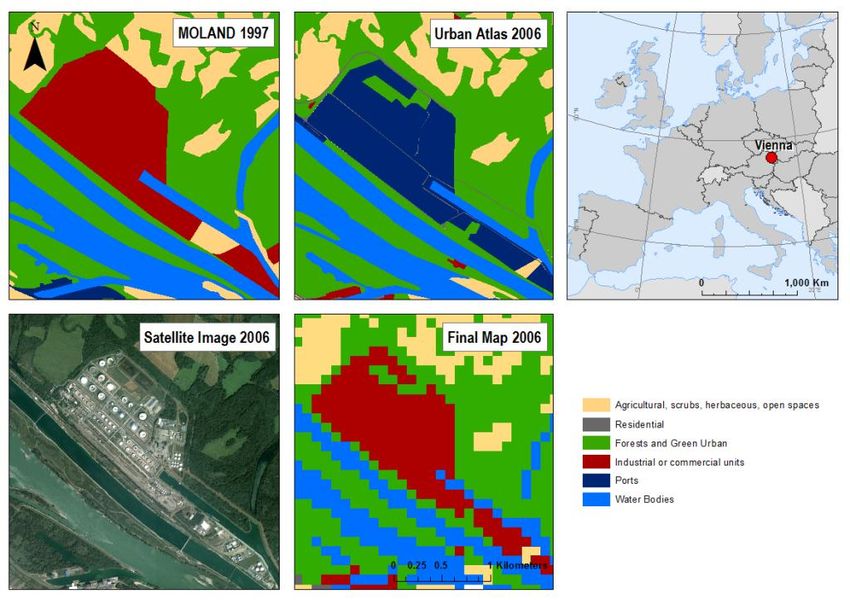
in the merged geo-database. The land use/cover classifications in both datasets were re-classified
accordingly.

Table 3. Land use classification used in the combined geo-database.

 Code Description
 1 Urban residential
 2 Ports
 3 Airports
 121 Industrial or commercial units
 99 Agricultural, scrubs, herbaceous, open spaces
 431 Forests and Green Urban
 5 Water Bodies

Despite the common interpretation guidelines between MOLAND and Urban Atlas (both based on CLC),
some classification inconsistencies were detected. A complete correction of such inconsistencies would
require a thorough check of each land use polygon of each city. Because such manual check was
unfeasible due to time and resource constraints, a semi-automatic verification procedure was
implemented in order to remove the major classification inconsistencies between the two input
datasets.

The verification procedure included two main screenings implemented for each city. At first, the land
use shares were calculated for each time step, and then plotted as stacked bar charts against time. This
allowed to visually perceive trends in land use changes for each city (e.g. steady increase of urban areas
while decreasing agricultural areas), and detect anomalous peaks or dips in land use shares over time.
Second, eventual peaks or dips in land use shares were further inspected on the map, thus allowing to
check whether such ‘anomalies’ were the result of actual land use changes or, on the contrary, the
result of classification inconsistencies. Few major inconsistencies were detected, and in all cases
occurring in the transition between late-1990s (MOLAND) and 2006 (Urban Atlas). Land use polygons
with inconsistent classification were checked against ancillary information from available web sources
(Google Maps, Open Street Maps) in order to determine the most plausible classification according to
the CLC mapping guide (Büttner et al. 2006). Figure 4 depicts an example of a particular site in Vienna
where a large infrastructure was classified as ‘industrial or commercial unit’ in the MOLAND dataset and
as ‘port’ in the Urban Atlas dataset. A closer inspection revealed that the site was in fact used as an oil
refinery with some docking facilities for ships. Thus, the original classification from the MOLAND dataset
was kept.

The figure also reveals a higher degree of geometrical generalization of the land use polygons pertaining
to the MOLAND dataset. This stems from the different minimum mapping units used in both datasets: as
already mentioned, MOLAND has a minimum mapping unit of 1 hectare for artificial surfaces and 3
hectares for all other land use/cover types, while the Urban Atlas uses 0.25 and 1 hectares respectively.

 12

An additional pre-processing procedure was therefore carried out in order to harmonize as most as
possible the spatial resolution in an automated way. The information from the Urban Atlas had to be
generalized to fit the coarser resolution of the MOLAND dataset, as the inverse is conceptually not
possible. All maps were converted from the native vector data format to raster format at 100x100 meter
resolution (1 hectare). In the case of the Urban Atlas, the artificial land cover polygons of less than 1
hectare were filtered out prior to ‘rasterization’. Then, the polygons were converted to raster format
ensuring that in each 1 hectare pixel the land use class with more than 50% of the land share was
recorded. In all other cases, the land use class was determined by the dominant surrounding land use, or
majority rule (i.e. the land use class with highest number of surrounding pixels). This ensured a full
match of minimum mapping units for artificial land uses between the two data sources.

Finally, the raster map for 2006 was again processed in order to remove non-artificial patches of less
than 3 hectares (i.e. three pixels). This was done by applying a raster function which groups all
contiguous pixels of the same land use class. All the groupings of one or two pixels were removed and
replaced by the dominant surrounding land use class using, again, the majority rule.

This processing chain removed most of the noise and mapping artefacts that often result when data at
different resolutions are mixed. It also guaranteed that the minimum mapping unit of 1 and 3 hectares
were respected, allowing more smooth and plausible land use transitions for the whole time-series.

Figure 4. Example of thematic and spatial harmonization between the MOLAND and UA data sets for a specific site
in Vienna, Austria.

 13

All the land use/cover data were compiled in a geo-database which was structured in a simple way to
allow easy and quick querying by different users (figure 5). The data are organized per city and per year,
and available in both raster and vector versions. In the raster files, only the land use/cover categories as
found in table 3 are recorded. The vector files, in addition to the land use/cover categories, contain
information on the area and perimeter of each polygon feature. Representation files with colour scheme
were prepared and complement the geo-database.

The final pre-processing step consisted of adding an estimate of total population for each city and time-
step. Population was therefore estimated based on data of population at commune level for a long time-
series (1960-2010, in ten-year intervals) that has been recently generated internally at the European
Commission. The adequate calculations were performed in order to adjust the original population data
to the spatial and temporal mapping coverage of each city. For example, linear interpolation was applied
to infer population for inter-decennial time-steps whenever the MOLAND and Urban Atlas land
use/cover maps did not match temporally the original population data source.

Subsequent post-processing and analytical operations, such as the ones presented in following section
of this paper, build upon this geo-database and associated population data.

Figure 5. Structure of the final geo-database.

 14

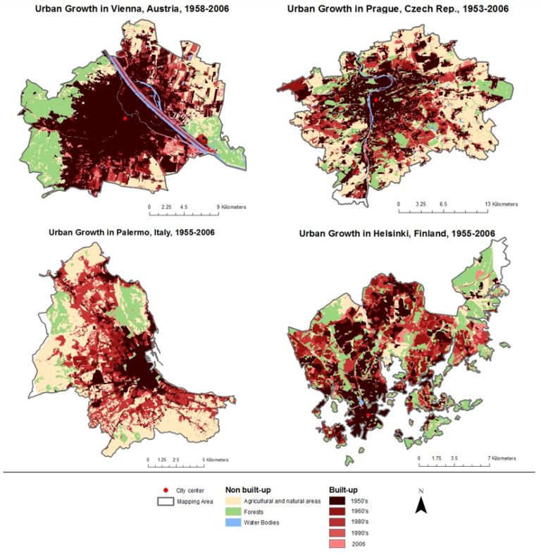
4. Urban expansion in European cities. Exploring the MOLAND-UATL
time series
The results presented in this section are shown mainly as example of what can be retrieved from the
new geo-database. For illustration purposes, figures 6 and 7 depict the urbanization process since the
mid-20th century for Vienna (Austria), Prague (Czech Republic), Palermo (Italy) and Helsinki (Finland). As
it can be observed, the four cities show very different urban morphology and growth dynamics. For
example, Vienna has been expanding at a steady pace, as opposed to Prague, Helsinki and Palermo
which had an early fast growth period followed by lower pace.

Table 4 shows a brief characterization of 29 cities under the focus of this paper. It summarizes the
mapping area per city, the population, population density and built-up area for 1950’s and 2006 and
corresponding percentage change. Copenhagen, Dublin, Duisburg, Essen, Milano, Mulheim, Nicosia,
Oberhausen, and Porto reveal a population decrease. Overall, population density in Europe is
decreasing. This phenomenon had been already observed by Ingram in 1998.

There are various types of density as well as many ways and scales to measure it (Burton 2000; Chin
2002; Churchman 1999). Having the land use per year and the corresponding population, it was then
possible to calculate the ‘net population density’, as suggested by Frenkel (2008). This means that only
artificial areas, and in particular the ones associated with residential uses, were used as denominator for
population density. This provides a more accurate and realistic figure of the actual population density
because it is not biased by size of the study area.

As demonstrated by Kasanko et al. in 2006, when plotting population and built-up areas in relative
terms, all cities are above the blue diagonal line (see figure 8). This line represents a situation of even
growth of population and built-up, that is, built-up areas growing at the same pace as population. Cities
above that have experienced faster growth of built-up areas in respect to the growth of population. The
further the city is located above the line, the larger is the gap in between the two growth rates. The
black diagonal line indicates the ordinary least square between the two variables. With a Pearson’s R-
squared of 0.43 and a p-value of 0.0001, there is a clear positive effect of population growth in the built-
up growth. The slope of 1.64 indicates that for each additional percent point of population, an additional
1.64 percent point of built-up growth can be expected. Even in the cases where population decreased,
built-up change was always positive. Haase (2013) also found this growth difference across European
cities.

 15

Figure 6. Urban expansion in Vienna, Prague, Palermo, and Helsinki between 1950 and 2006.

 16

Figure 7. Share of different land use/cover types for Vienna, Prague, Palermo, and Helsinki between 1950 and 2006.

The dotted lines in figure 8 reflect the median for each of the variables, being 15.5% for population and
102.6% for built-up. This last value is mainly driven by Southern cities. Cities belonging to other
geographical blocks show a much less pronounced urban expansion in the 1950’s – 2006 period, with
the exceptions of Grenoble and Bratislava. The latter cities and those from the South block may be
experiencing a fast built-up growth due to a lower than average starting point, in which case they have
been catching up with the overall trend. Rising living standards, changing of habitation preferences
(single houses preferred over blocks or flats), and reduction of the average household sizes (smaller
families) all contribute to more space per person required. Land use policies (attitude towards
compact/sprawled urbanization, etc.) are known to be an important factor as well (Kasanko et al. 2006).
Higher motorization levels (more private motor vehicles and extended road infrastructure) have been
contributing directly to ease of access to and from city centres, allowing people to spread spatially to
suburban areas (Huang et al. 2007; Aguayo et al. 2007), where price of land is lower.

 17

Table 4. Population, built-up area and population density in 1950 and 2006 for the cities mapped in the combined geo-database.

City Block Mapping Population Population Change Urban Urban Urban Population Population Change Pop.
 2
 Area (km ) 1950’s 2006 Pop. 1950- residential residential residential Density Density Density
 (habitants) (habitants) 2006 1950’s 2006 1950’s – 1950’s 2006 1950-2006
 2 2 2 2 2 2
 (habitants) (km ) (km ) 2006 (km ) (habs/km ) (habs/km ) (habs/km )
Bilbao South 38.55 205,174 351,443 146,269 5.87 12.27 6.40 34,981 28,642 -6339
Bratislava East 352.34 206,165 420,450 214,285 27.59 68.11 40.52 7,473 6,173 -1300
Brussels West 162.34 441,436 506,703 65,267 75.19 95.64 20.45 5,871 5,298 -573
Copenhagen North 98.36 897,297 604,952 -292,345 53.80 54.35 0.55 16,679 11,130 -5549
Dresden East 326.57 530,403 500,433 -29,971 58.35 96.54 38.19 9,091 5,184 -3907
Dublin West 117.53 423,956 498,826 74,870 43.39 69.95 26.57 9,772 7,131 -2641
Duisburg West 117.61 392,872 280,936 -111,937 39.43 47.60 8.17 9,964 5,902 -4062
Essen West 130.80 538,302 403,836 -134,467 56.07 70.15 14.09 9,601 5,756 -3844
Faro* South 103.55 15,863 29,398 13,535 3.18 9.28 6.10 4,983 3,168 -1815
Gothenburg North 54.34 85,320 103,763 18,443 19.75 26.78 7.03 4,321 3,874 -446
Grenoble West 195.14 131,918 385,547 253,629 20.74 15.54 -5.20 6,360 5,915 -445
Helsinki North 204.33 389,445 572,012 182,567 40.38 86.97 46.59 9,644 6,577 -3067
Heraklion South 29.33 69,364 102,407 33,044 4.31 65.19 60.88 16,103 6,591 -9512
Lyon West 310.00 793,421 1,088,733 295,312 80.33 151.96 71.63 9,878 7,165 -3175
Marseille South 237.94 673,104 831,362 158,259 54.38 90.33 35.95 12,379 9,204 -3175
Milan South 181.40 1,450,769 1,253,380 -197,389 60.82 93.85 33.04 23,854 13,354 -10500
Mulheim West 43.99 124,062 118,215 -5,847 19.57 24.60 5.04 6,341 4,805 -1536
Munich West 310.87 975,030 1,281,705 306,674 107.99 156.46 48.47 9,029 8,192 -837
Nicosia South 76.00 19,480 14,567 -4,913 13.62 39.86 26.24 1,431 365 -1065
Oberhausen West 58.23 218,128 179,075 -39,053 25.73 31.93 6.20 8,477 5,608 -2869
Olhao* South 104.77 28,175 43,009 14,834 3.04 12.05 9.01 9,280 3,571 -5710
Padua South 93.00 172,102 205,753 33,651 15.16 38.39 23.23 11,351 5,359 -5993
Palermo South 157.65 545,099 673,411 128,312 18.18 60.39 42.21 29,986 11,151 -18835
Porto South 41.29 302,794 250,978 -51,816 16.88 25.36 8.47 17,933 9,897 -8036
Prague East 491.84 1,126,362 1,201,167 74,806 105.35 155.73 50.38 10,691 7,713 -2978
Setubal South 21.22 18,857 33,656 14,799 1.79 7.89 6.10 10,527 4,265 -6262
Tallinn East 158.98 276,757 397,074 120,318 38.54 55.44 16.90 7,181 7,162 -19
Venice South 126.82 204,946 206,865 1,919 12.64 31.31 18.67 16,211 6,607 -9604
Vienna West 414.85 1,629,460 1,631,943 2,483 139.11 167.10 27.99 11,714 9,766 -1947
Average - 164,125,184 475,630 488,676 13,045 40.04 64.17 24.13 11,879 7,615 -4,264
Minimum - 21,224,698 18,857 14,567 -292,345 1.79 7.89 -5.20 1,431 365 -18,835
Maximum - 491,836,459 1,629,460 1,631,943 306,674 139.11 167.10 71.63 34,981 28,642 -19
Std.Deviation - 120,574,702 418,351 425,145 139,063 34.38 46.12 19.22 7,225 4,803 3,970

* Data refers to 1960 to 2006.

 18

Figure 8. Population and built-up growth between 1950 and 2006.

By plotting the growth of built-up areas against the decrease of population density, cities were classified
in four main groups according to their position above or below the respective means (dotted lines in
figure 9). Similar techniques have been applied in previous attempts to measure urban sprawl using
scatterplots (Frenkel and Ashkenazi 2008; Altieri et al. 2014). In figure 9, cities falling in the upper right
quadrant are characterized by very strong urban dynamics, with high built-up growth rates but great
overall decrease of population density (high change). Cities in the opposite quadrant show a much more
stable behaviour during the same time span (low change). On the upper left quadrant are cities affected
by low degree of built-up growth and relevant decrease of population density, which may indicate a very
low urbanization activity, i.e. few people attracted to the city core (partial change). Finally, remainder
cities in the lower right quadrant show high built-up growth-rates and little population density decrease,
which indicates strong urbanization dynamics and attractiveness (partial change). It is remarkable that
the upper right corner is exclusively composed by cities located in the Southern/Mediterranean area of
Europe, while the cities from the West Europe show the most moderate built-up growth rates. This
confirms what has been already mentioned: cities in the Southern area were catching up the most
developed ones of the West and North during the last quarter of the 20th century. In the map of figure
10 each city is colour-coded according to the classification derived from this analysis.

 19

Figure 9. Increase in built-up areas and decrease in population density between 1950 and 2006.

Figure 10. Typology of cities according to the scatter-plot classification.

 20

5. Discussion and conclusions regarding the generation of urban
historical time series data
Long time-series of land use/cover maps are rare due to various reasons. Efforts to consistently map and
track land use changes intensified only by the end of the 20th century, as interest for landscape,
urbanization and the environment started to gain momentum, and as satellite imagery and Geographical
Information Systems became widespread. Currently, at the European level, there are several initiatives
to monitor land use changes, the CORINE Land Cover project being one of the most acknowledged.
However, to study more long-term dynamics, and learn from more distant past, longer time-series are
essential, yet very little data exist. Even the CLC starts recording land use changes only from 1990
onwards.

The MOLAND geo-database, as thoroughly described earlier in this paper, is a unique project that
allowed to gather data on land use/cover changes for an extended period that spans from circa 1950 to
late-1990s, for a sample of more than 30 urban areas across Europe. Unfortunately this remarkable
initiative was not continued (let alone expanded, as it fully deserved). More recently, the Urban Atlas
project mapped the land use in 2006 for over 300 European cities with considerable spatial resolution,
but with low thematic detail.

In this paper we identified the opportunity to merge both geo-datasets to create an extended urban
time-series covering the period 1950-2006. Such effort revealed a number of challenges that had to be
tackled and which related to spatial and thematic inconsistencies between MOLAND and Urban Atlas. A
workflow and methodology were set-up in order to harmonize both datasets and make them consistent
and comparable. This required a number of trade-offs which resulted in a loss of some thematic detail
from MOLAND, and a decrease of the spatial resolution from Urban Atlas. Besides this unavoidable
trade-off, other limitations of the final product are referred next.

As described in section 3, a set of semi-automatic verifications and GIS procedures were applied to
harmonize both the thematic and spatial detail of the two datasets. A screening and correction of the
major thematic inconsistencies (e.g. the same land feature classified differently in MOLAND and Urban
Atlas datasets) were implemented, ensuring that the recorded land use changes between late-1990s
and 2006 are actual land use changes and not the result of issues with image interpretation rules.
Nonetheless, because not every polygon was checked, smaller inconsistencies might still be present. In
addition, a set of generalization rules were as well applied to the Urban Atlas in order to adjust it to the
coarser minimum mapping units of the MOLAND dataset. While the applied GIS procedures ensured a
nominal compliance with the minimum mapping units, those rules were applied automatically, without
actual checking of the satellite imagery of 2006. In fact, whenever a land use feature from the Urban
Atlas was below the minimum mapping unit, it was filtered out and replaced by the dominant
surrounding land use class. This sensible rule should apply in the vast majority of the cases, but might
not fit in all situations, thus adding to overall uncertainty. For example, when several land use classes
are in the vicinity of a removed land use feature, closer inspection of the neighbouring land uses and
their spatial arrangements would guarantee an even more pondered and accurate decision regarding
the actual dominant land use. The highly aggregated land use nomenclature used (with only 7 broad

 21

land use classes), reduced considerably the thematic detail, but also limited a great deal of uncertainty.
In any case, due to the mentioned potential sources of uncertainty, the merged time-series is not
recommended to pixel by pixel analysis. Change detection, for instance, should be done at larger scale.

Despite the above mentioned trade-offs and limitations, this project resulted in a new, integrated geo-
database comprised of a long historical time-series of urban land uses for nearly 30 European cities. This
dataset was further enriched by including population data for each time-step. A first, exploratory
analysis of the results demonstrated the usefulness and relevance of this mapping product for urban
studies. The covered cities were classified according to their long-term record of land use changes,
allowing the identification of trends and patterns in urbanization.

The work here presented is part of a broader line of research. Following stages will include more in-
depth study of past and future urbanization processes and dynamics, for which some concrete technical
challenges lie ahead: new and more robust indicators for characterizing urban growth are being
developed; finer population maps will be produced by downscaling population counts to grid level. In
addition, the information compiled and structured in this geo-database could be used to improve the
calibration of land use models at EU-level (Lavalle et al. 2011). Finally, the upcoming update of Urban
Atlas, covering 2012, can be integrated as an additional new time-step in MOLAND-Urban Atlas geo-
database.

This work permitted as well to highlight the importance of the availability of long and consistent land
use time-series data, which are still lacking worldwide, and would definitely contribute to the land
change science (Rindfuss et al. 2004). The harmonization effort herein presented could only be carried
out at the cost of detail, and for a relatively small sample of cities. This should therefore serve as a
reminder of what could have been done if, in the past, more had been invested into mapping. To avoid
such regrets in the future, systematic and consistent tracking of land use changes should be a concern of
researchers and authorities.

6. Weighted Urban Proliferation Index
Weighted Urban proliferation (WUP) is an index, proposed by Jaeger and Schwick (2014) to quantify
urban sprawl. It is based on the following definition of urban sprawl: “the more area built over in a given
landscape (amount of built-up area) and the more dispersed this built-up area in the landscape (spatial
configuration), and the higher the uptake of built-up area per inhabitant or job (lower utilization
intensity in the built-up area), the higher the degree of urban sprawl”. The WUP is calculated as a
combination of three different elements taking into consideration (1) the degree of urban penetration
(incorporating the distance between built-up cells), (2) the density of built-up area and (3) the
population present in this built-up area.

 22

6.1 Methods

The calculation of the weighted urban proliferation (WUP), as a quantification of urban sprawl, was
adapted from the method published by Jaeger and Schwick (2014). The WUP indicator was calculated,
for each urban pixel (i) of EU-wide maps at a 100 * 100 meter resolution, by making use of the equations
below.

 = × 1 × 2 

  Calculation of the degree of urban permeation (UP)

 ∗ 2
 = ×
 TLA
Where TLA is the total landscape area

 Cs: cell size of the raster (100m)

 ni: number of built in cell surrounding cell i within the specified horizon of perception

  Calculation of the degree of urban dispersion (DIS)
 
 + ∑ (√2.0 × + 1.0 − 1.0)
 =0
 =
 
Where = √0.97428 − + 1.046 − 0.996249

And = √( − )2 + ( − )2 × 

Where Dij : is the distance from cell i to cell j

 Xi abscissa raster coordinate of cell i

 Yi ordinate raster coordinate of cell i

Figure 11 illustrates the computations performed in the calculations of the distance between urban cells
within the horizon of perception.

 23

Figure 11. Illustration of the cell distance calculation procedure.

  Calculation of W2 (scaling function based on population):
 1
 2 =
 2.8912029
 1 + ( )

Where: Popi: population at cell i

 UD = 67.065

  Calculation of W1 (scaling function based on the density of built-up area):
 0.5 − 1.5
 1 = 1.5 +
 11.02135
 1 + 44.97

The approach differed from (Jaeger & Schwick, 2014) in the following points:

The WUP was calculated for each 100*100 meter pixel of urban land-use (rather than aggregated at a
broader regional level). As the value of WUP depends on the “Area Built-up / Area Reporting Unit” ratio
(which differs greatly from our study to the one of Jaeger) a parameter adjustment was made to scale
the WUP to a value range similar to that of Jaeger’s.

Here a horizon of perception of 10 km was used, rather than the 2km used in the Jaeger and Schwick
(2014) study. This distance was selected to take into account larger commuting distances.

 24

Due to the lack of spatially explicit EU wide employment data, population density was substituted for
the “inhabitants + jobs” variable that Jaeger & Schwick use to compute Utilization density.

The calculation of W2 and W1 were simplified into four parameters logistics regressions to allow for
easier customizations by the user.

To deal with the very large number of computations associated with the calculation of the weighted
urban proliferation at the EU 28 scale, a set of computer scripts were developed to “smart tile” the
dataset into smaller samples more easy to handle.

6.2 Preliminary results and interpretation

The WUP was calculated for the year 2010, 2020 and 2030 for the reference (Lavalle, 2013) and compact
policy scenario (Batista e Silva, 2013).

A preliminary “visual analysis” of the results at pixel level (see Figure 112) suggests that the calculated
WUP values follow a spatial pattern and value range similar to that of Jaeger and Schwick (2014).
Densely populated area display low WUP values (green color in figure 12) while less dense more sparsely
populated area display higher values (red color).

 WUP (UPU/m2)

Figure 112: Pixel WUP for 2010 reference scenario for W. Vienna, in Austria.

 25

An application of the UP and DIS component of the WUP indicator to historical time series (Figure 13) of
the development of European city also provided results in par with the observed specific development
of urban sprawl for each city

 UP Historical Timeseries
 35

 30

 25

 20

 15

 10

 5

 0
 1940 1950 1960 1970 1980 1990 2000 2010

 Vienna Porto Bilbao Bratislava
 a)

 DIS Historical Timeseries
 49
 48.5
 48
 47.5
 47
 46.5
 46
 45.5
 45
 44.5
 44
 43.5
 1940 1950 1960 1970 1980 1990 2000 2010

 Vienna Porto Bilbao Bratislava
 b)
Figure 13: Time series of changes in UP (a) and DIS (b) aggregated at city level for 4 European cities.

 26

An application of the WUP indicator, aggregated at the scale of large urban zone (Figure 113 and Figure
14) can be used to estimate the potential effectiveness of policies to influence future urban sprawl.
Figure 14 and 15 provide an illustration of changes in WUP from 2010 to 2020 for 2 policy scenarios at
the EU 28 scale.

Figure 113: WUP aggregated for large urban zone of changes in WUP between 2010 and 2030 under a reference
policy scenario.

 27

Figure 114: WUP aggregated at country level and representing changes in WUP between 2010 and 2030 under a
reference policy scenario.

Such outputs have the potential be used to evaluate the impact of different policies on the structure of
cities, define urban sprawl thresholds, special intervention and restricted building areas. Further testing
of this approach is ongoing.

7. Conclusions and future steps

The work herein presented is part of a wider framework that is set up to examine policy impacts and
evaluate options to improve the effectiveness of EU action. The core of the framework is an integrated
modelling platform – called LUISA (Land Use-based Integrated Sustainability Assessment modelling
platform) – that is based upon the integration of coherent databases and interconnected models. The
development of European wide databases which are thematically and cartographically consistent is a
crucial element for the evaluation of historical trends and evolutions of urban areas. The merging of the
MOLAND and Urban Atlas datasets provides a unique and inestimable source of information on the
status of European cities. The development of indicators and indexes of urban development that are
able to describe complex processes with intuitive representation is a further key element of the
framework. The here described WUP indicator is an example of one of those indicators, which is now
fully and dynamically integrated in LUISA and will be employed for the evaluation of past and future
trends of urbanisation in Europe.

 28

8. References
Aguayo, MI, Wiegand T, Azócar GD, Wiegand K, Vega CE. 2007. Revealing the Driving Forces of Mid-
Cities Urban Growth Patterns Using Spatial Modeling: a Case Study of Los Ángeles, Chile. Ecology &
Society 12(1): 13.

Altieri L, Cocchi D, Pezzi G, Scott EM, Ventrucci M. 2014. Urban sprawl scatterplots for Urban
Morphological Zones data. Ecological Indicators 36: 315-323.

Bai X, Chen J, Shi P. 2012. Landscape urbanization and economic growth in China: positive feedbacks and
sustainability dilemmas. Environmental Science & Technology 46: 132-139.

Barranco RR, Batista e Silva F, Marin Herrera M, Lavalle C. 2014. Integrating the MOLAND and the Urban
Atlas Geo-databases to Analyze Urban Growth in European Cities, Journal of Map & Geography Libraries:
Advances in Geospatial Information, Collections & Archives, 10:3, 305-328

Barredo JI, Kasanko M, McCormick N, Lavalle C. 2003. Modelling dynamic spatial processes: simulation
of urban future scenarios through cellular automata. Landscape and Urban Planning, 64(3): 145-160.

Batista e Silva F, Marques TS. 2010. The Study of Urban Growth through Multi‐temporal Cartography
and Spatial Indicators: the case of Porto Region, Portugal. 17th Conference International Seminar on
Urban Form (ISUF), 20 -23 August 2010, Hamburg and Lubeck, Germany.

Batista E Silva F, Lavalle C, Jacobs C, Ribeiro Barranco R, Zulian G, Maes J, Baranzelli C, Perpiña Castillo C,
Vandecasteele I, Ustaoglu E, Lopes Barbosa A, Mubareka S. 2013. Direct and Indirect Land Use Impacts
of the EU Cohesion Policy. Assessment with the Land Use Modelling Platform. EUR 26460 EN.
Luxembourg (Luxembourg): Publications Office of the European Union; JRC87823

Batty M. 2013. A Theory of City Size. Science 340(6139): 1418-1419.

Bettencourt LMA. 2013a. The origins of scaling in cities. Science 340(6139): 1438-1441.

Bettencourt, LM, Lobo J, Helbing D, Kühnert C, West GB. 2007. Growth, innovation, scaling, and the pace
of life in cities. Proceedings of the National Academy of Sciences, 104(17): 7301-7306.

Bloom DE, Canning D, Fink G. 2008. Urbanization and the wealth of nations. Science 319(5864): 772-775.

Burchell RW, Shad NA, Listokin D, Phillips H, Downs A, Seskin S, Davis J, Moore T, Helton D, Gall M. 1998.
The costs of sprawl-revisited. Report 39, Transit Cooperative Research Program (TCRP) Transportation
Research Board, National Research Council, Washington, DC. pp. 83-125.

Burton E. 2000. The compact city: just or just compact? A preliminary analysis. Urban studies 37(11):
1969-2006.

Büttner G, Feranec G, Jaffrain G. 2006. CORINE Land Cover Nomenclature Illustrated Guide – Addendum
2006. Unpublished Report. 84 p.

 29