Insights into atmospheric oxidation processes by performing factor analyses on subranges of mass spectra - ACP
←
→
Page content transcription
If your browser does not render page correctly, please read the page content below
Atmos. Chem. Phys., 20, 5945–5961, 2020
https://doi.org/10.5194/acp-20-5945-2020
© Author(s) 2020. This work is distributed under
the Creative Commons Attribution 4.0 License.

Insights into atmospheric oxidation processes by performing factor
analyses on subranges of mass spectra
Yanjun Zhang1 , Otso Peräkylä1 , Chao Yan1 , Liine Heikkinen1 , Mikko Äijälä1 , Kaspar R. Daellenbach1 , Qiaozhi Zha1 ,
Matthieu Riva1,2 , Olga Garmash1 , Heikki Junninen1,3 , Pentti Paatero1 , Douglas Worsnop1,4 , and Mikael Ehn1
1 Institute for Atmospheric and Earth System Research/Physics, Faculty of Science,
University of Helsinki, Helsinki, 00014, Finland
2 Univ. Lyon, Université Claude Bernard Lyon 1, CNRS, IRCELYON, 69626, Villeurbanne, France
3 Institute of Physics, University of Tartu, Tartu, 50090, Estonia
4 Aerodyne Research, Inc., Billerica, MA 01821, USA

Correspondence: Yanjun Zhang (yanjun.zhang@helsinki.fi)

Received: 18 September 2019 – Discussion started: 28 November 2019
Revised: 23 March 2020 – Accepted: 26 March 2020 – Published: 19 May 2020

Abstract. Our understanding of atmospheric oxidation              is included for PMF analysis. In addition to the main findings
chemistry has improved significantly in recent years, greatly     listed above, several other benefits compared to traditional
facilitated by developments in mass spectrometry. The gen-        methods were found.
erated mass spectra typically contain vast amounts of infor-
mation on atmospheric sources and processes, but the identi-
fication and quantification of these is hampered by the wealth
of data to analyze. The implementation of factor analysis         1   Introduction
techniques have greatly facilitated this analysis, yet many at-
mospheric processes still remain poorly understood. Here,         Huge amounts of volatile organic compounds (VOCs) are
we present new insights into highly oxygenated products           emitted to the atmosphere every year (Guenther et al., 1995;
from monoterpene oxidation, measured by chemical ioniza-          Lamarque et al., 2010), which play a significant role in at-
tion mass spectrometry, at a boreal forest site in Finland in     mospheric chemistry and affect the oxidative ability of the
autumn 2016. Our primary focus was on the formation of            atmosphere. The oxidation products of VOCs can contribute
accretion products, i.e., dimers. We identified the formation     to the formation and growth of secondary organic aerosols
of daytime dimers, with a diurnal peak at noontime, despite       (Kulmala et al., 2013; Ehn et al., 2014; Kirkby et al., 2016;
high nitric oxide (NO) concentrations typically expected to       Troestl et al., 2016), affecting air quality, human health, and
inhibit dimer formation. These dimers may play an impor-          climate radiative forcing (Pope et al., 2009; Stocker et al.,
tant role in new particle formation events that are often ob-     2013; Zhang et al., 2016; Shiraiwa et al., 2017). Thanks to
served in the forest. In addition, dimers identified as com-      the advancement in mass spectrometric applications, like the
bined products of NO3 and O3 oxidation of monoterpenes            aerosol mass spectrometer (AMS) (Canagaratna et al., 2007)
were also found to be a large source of low-volatility vapors     and chemical ionization mass spectrometry (CIMS) (Bertram
at night. This highlights the complexity of atmospheric oxi-      et al., 2011; Jokinen et al., 2012; Lee et al., 2014), our capa-
dation chemistry and the need for future laboratory studies on    bility to detect these oxidized products, as well as our under-
multi-oxidant systems. These two processes could not have         standing of the complicated atmospheric oxidation pathways
been separated without the new analysis approach deployed         in which they take part, has been greatly enhanced.
in our study, where we applied binned positive matrix fac-           Monoterpenes (C10 H16 ), one major group of VOCs emit-
torization (binPMF) on subranges of the mass spectra rather       ted in forested areas, have been shown to be a large source
than the traditional approach where the entire mass spectrum      of atmospheric secondary organic aerosol (SOA). The ox-
                                                                  idation of monoterpenes produces an abundance of differ-

Published by Copernicus Publications on behalf of the European Geosciences Union.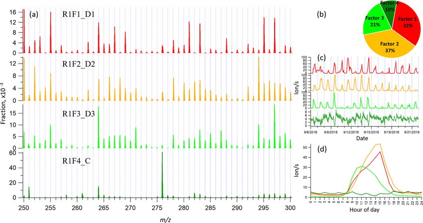
5946                                                              Y. Zhang et al.: Insights into atmospheric oxidation processes

ent oxidation products (oxygenated VOC, OVOC), includ-                monoterpene ozonolysis) depending on the application and
ing highly oxygenated organic molecules (HOMs) with mo-               ability to identify spectral signatures (Yan et al., 2016; Zhang
lar yields in the range of a few percent, depending on the spe-       et al., 2017).
cific monoterpene and oxidant (Ehn et al., 2014; Bianchi et              In the vast majority of these PMF applications to mass
al., 2019). Recent chamber studies have greatly advanced our          spectra, the mass range of ions has been maximized in order
knowledge of formation pathways for monoterpene HOM                   to provide as much input as possible for the algorithm. This
products, e.g., monomers (typically C9−10 H12−16 O6−12 ) and          approach was certainly motivated in the early application of
dimers (typically C19−20 H28−32 O8−18 ). Dimers, as shown by          PMF by, for example, offline filters, with chemical informa-
previous studies, can contribute to new particle formation            tion of metals, water-soluble ions, and organic carbon and el-
(NPF) (Kirkby et al., 2016; Troestl et al., 2016; Lehtipalo           emental carbon (OC and EC), where the number of variables
et al., 2018), and they are thus of particular interest.              is counted in tens, and the number of samples in tens or hun-
   In nearly all atmospheric oxidation chemistry, peroxy rad-         dreds (Zhang et al., 2017). However, with gas-phase CIMS,
icals (RO2 ) are the key intermediates (Orlando and Tyndall,          we often have up to a thousand variables, with hundreds or
2012). They form when VOCs react with oxidants like ozone,            even thousands of samples, meaning that the amount of data
or the hydroxyl (OH) or nitrate (NO3 ) radicals, while their          itself is unlikely to be a limitation for PMF calculation. In this
termination occurs mainly by bimolecular reactions with ni-           work, we aimed to explore potential benefits of dividing the
tric oxide (NO), hydroperoxyl (HO2 ), and/or other RO2 .              spectra into subranges before applying factorization analy-
RO2 + R0 O2 reactions can form ROOR0 dimers (Berndt et                sis. This approach was motivated by several issues, which we
al., 2018a, b), and this pathway competes with RO2 + NO               expected to be resolvable by analyzing several mass ranges
reactions, meaning that NO, formed by photolysis of NO2 ,             separately. Firstly, the loss rate of OVOCs by condensation
can efficiently suppress dimer formation, as also seen from           is strongly coupled to the molecular mass (Peräkylä et al.,
atmospheric HOM observations (Ehn et al., 2014; Yan et al.,           2020), likely giving very different behaviors for the high and
2016). Mohr et al. (2017) also reported daytime dimers in the         low mass ranges, even when produced by the same source.
boreal forest in Finland, coinciding with NPF events. A bet-          Second, dimers are a product of two RO2 radicals, which can
ter understanding of the formation of these daytime dimers            have different sources, meaning that they may have temporal
would assist elucidating NPF and particle growth mecha-               profiles unlike anything observable for monomers. Finally, if
nisms.                                                                one mass range contains much less signal than another, it will
   At night, nitrogen oxides can also impact the oxidation            have very little impact on the final PMF results.
pathways when NO2 and O3 react to form NO3 radicals that                 In this study, we applied PMF analysis on three differ-
can oxidize monoterpenes. NO3 radicals are greatly reduced            ent mass ranges of mass spectra of OVOCs measured by a
during daytime due to photolysis and reactions with NO re-            chemical ionization atmospheric pressure interface time-of-
ducing their lifetime to a few seconds (Ng et al., 2017). Yan         flight (CI-APi-TOF; Jokinen et al., 2012) mass spectrometer
et al. (2016) reported nighttime HOMs initiated by NO3 in             in the Finnish boreal forest. We utilized our recently pro-
the boreal forest in Finland, but to our knowledge there have         posed new PMF approach, binPMF, to include as much of
been no laboratory studies on HOM formation from NO3 ox-              the high-resolution information in the mass spectra as possi-
idation of monoterpenes. However, there have been several             ble in a robust way (Zhang et al., 2019). We show the bene-
studies looking into the SOA formation in these systems,              fits of the subrange PMF approach to better separate chemi-
finding that certain monoterpenes, like β-pinene, have very           cal sources by reducing disturbance from variable loss terms
high SOA yields, while the most abundant monoterpene, α-              of the OVOCs. Much of the analysis focuses on dimer for-
pinene, has negligible SOA forming potential. It remains an           mation pathways and the role of different nitrogen oxides in
open question as to what the role of NO3 radical oxidation of         these pathways. We find that both daytime dimers and dimers
monoterpenes, and the observed NO3 -derived HOMs, in the              resulting from the combination of different oxidants can be
nighttime boreal forest is. Identification of these processes         separated with the subrange approach but not with the PMF
in the ambient environment is fundamental for better under-           applied to the full mass range. We believe that this study will
standing of NPF and SOA.                                              provide new perspectives for future studies analyzing gas-
   The recent development of CIMS techniques has allowed              phase CIMS data.
researchers to observe unprecedented numbers of OVOCs in
real time (Riva et al., 2019). This ability to measure thou-
sands of compounds is a great benefit, but it is also a large         2   Methodology
challenge for the data analyst. For this reason, factor analyt-
ical techniques have often been applied to reduce the com-            The focus of this work is on retrieving new information
plexity of the data (Huang et al., 1999), e.g., positive ma-          from mass spectra by applying new analytical approaches.
trix factorization, PMF (Paatero and Tapper, 1994; Zhang et           Therefore, we chose a dataset that has been presented earlier,
al., 2011). The factors have then been attributed to sources          though without PMF analysis, by Zha et al. (2018) and was
(e.g., biomass burning organic aerosol) or processes (e.g.,           also used in the first study describing the binPMF method

Atmos. Chem. Phys., 20, 5945–5961, 2020                                                 https://doi.org/10.5194/acp-20-5945-2020
Y. Zhang et al.: Insights into atmospheric oxidation processes                                                              5947

(Zhang et al., 2019). The measurements are described in           2.2   Positive matrix factorization (PMF)
more details below in Sect. 2.1, while the data analysis tech-
niques used in this work are presented in Sect. 2.2.              After the model of PMF was developed (Paatero and Tapper,
                                                                  1994), numerous applications have been conducted with dif-
2.1     Measurements                                              ferent types of environmental data (Song et al., 2007; Ulbrich
                                                                  et al., 2009; Yan et al., 2016; Zhang et al., 2017). By reducing
2.1.1    Ambient site                                             the dimensionality of the measured dataset, the PMF model
                                                                  greatly simplifies the data analysis process with no require-
The ambient measurements were conducted at the Station            ment for prior knowledge of sources or pathways as essential
for Measuring Ecosystem–Atmosphere Relations (SMEAR)              input. The main factors can be further interpreted with their
II in Finland (Hari and Kulmala, 2005) as part of the In-         unique or dominant markers (elements or masses).
fluence of Biosphere-Atmosphere Interactions on the Reac-            The basic assumption for PMF modeling is mass balance,
tive Nitrogen budget (IBAIRN) campaign (Zha et al., 2018).        which assumes that ambient concentration of a chemical
Located in the boreal environment in Hyytiälä, SMEAR II           component is the sum of contributions from several sources
is surrounded by coniferous forest and has limited anthro-        or processes, as shown in Eq. (1).
pogenic emission sources nearby. Diverse measurements of          X = TS × MS + R                                             (1)
meteorology, aerosol, and gas-phase properties are continu-
ously conducted at the station. Details about the meteorolog-     In Eq. (1), X stands for the time series of measured concen-
ical conditions and temporal variations of trace gases during     tration of different variables (m/z in our case), TS represents
the IBAIRN campaign are presented by Zha et al. (2018) and        the temporal variation of factor contributions, MS stands for
Liebmann et al. (2018).                                           factor profiles (mass spectral profiles), and R is the resid-
                                                                  ual as the difference of the modeled and the observed data.
2.1.2    Instrument and data                                      The matrices TS and MS are iteratively calculated by a least-
                                                                  squares algorithm utilizing uncertainty estimates to pursue a
Data were collected with a nitrate (NO−      3 )-based chemi-
                                                                  minimized Q value as shown in Eq. (2), where Sij is the es-
cal ionization atmospheric pressure interface time-of-flight      timated uncertainty, an essential input in the PMF model.
mass spectrometer (CI-APi-TOF, Jokinen et al., 2012) with               X X  Rij 2
about 4000 Th Th−1 mass-resolving power at ground level in        Q=                                                          (2)
                                                                                   Sij
September 2016. In our study, the mass spectra were aver-
aged to 1 h time resolution from 6 to 22 September for fur-       The PMF model was conducted by multilinear engine (ME-
ther analysis. We use the thomson (Th) as the unit for mass-      2) (Paatero, 1999) and interfaced with Source Finder (SoFi,
to-charge ratio, with 1 Th = 1 Da/e, where e is the elemen-       v6.3) (Canonaco et al., 2013). Signal-to-noise ratio (SNR)
tary charge. As all the data discussed in this work are based     was calculated as SNRij = abs (Xij )/abs (Sij ). When the
on negative ion mass spectrometry, we will use the absolute       signal-to-noise ratio (SNR) is below 1, the signal of Xij
value of the mass-to-charge ratio, although the charge of each    will be down-weighted by replacing the corresponding un-
ion will be negative. The masses discussed in this work in-       certainty Sij by Sij /SNRij (Visser et al., 2015). Future stud-
clude the contribution from the nitrate ion, 62, unless specif-   ies should pay attention to the potential risk when utilizing
ically mentioned. Furthermore, as the technique is based on       this method since down-weighting low signals element-wise
soft ionization with NO− 3 ions, any multiple charging effects    will create a positive bias in the data. Robust
                                                                                                                mode was  cho-
are unlikely, and therefore the reported mass-to-charge val-                                                      Rij
                                                                  sen in the PMF modeling, where outliers | Sij | > 4 were
ues in thomson can be considered equivalent to the mass of        significantly down-weighted (Paatero, 1997).
the ion in dalton (Da).
   The forest site of Hyytiälä is dominated by monoterpene        2.3   binPMF
emissions (Hakola et al., 2006). The main feature of previ-
ous CI-APi-TOF measurements in Hyytiälä (Ehn et al., 2014;        As a newly developed application of PMF for mass spec-
Yan et al., 2016) has been a bimodal distribution of HOMs,        tral data, binPMF has no requirement for chemical compo-
termed monomers and dimers, as they are formed of either          sition information while still taking advantage of the high-
one or two RO2 radicals, respectively. For the analysis in this   resolution (HR) mass spectra, saving effort and time (Zhang
study, we chose three mass-to-charge (m/z) ranges of 50 Th        et al., 2019). To explore the benefits of analyzing sepa-
each (Fig. 1), corresponding to regions between which we          rated mass ranges, we applied binPMF to the three sepa-
expect differences in formation or loss mechanisms. In addi-      rated ranges. The three ranges were also later combined for
tion to regions with HOM monomers and HOM dimers, one             binPMF analysis as a comparison with the previous results.
range was chosen at lower masses, in a region presumably          The PMF model requires both data matrix and error matrix
mainly consisting of molecules that are less likely to con-       as input, and details of the preparation of data and error ma-
dense onto aerosol particles (Peräkylä et al., 2020).             trices are described below.

https://doi.org/10.5194/acp-20-5945-2020                                           Atmos. Chem. Phys., 20, 5945–5961, 2020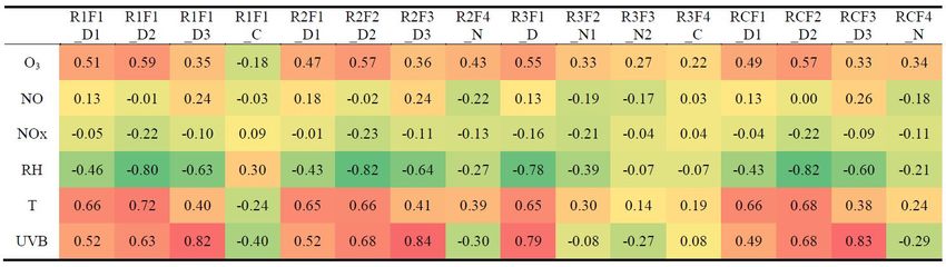
5948 Y. Zhang et al.: Insights into atmospheric oxidation processes
2.3.1 Data matrix 3 Results
Unlike normal unit mass resolution (UMR) or HR peak fit- 3.1 General overview of the dataset and spectrum
ting, in binPMF, the mass spectra are divided into small bins
after baseline subtraction and mass axis calibration. Linear During the campaign, in autumn 2016, the weather was over-
interpolation was first conducted on the mass spectra with all sunny and humid with average temperature of 10.8 ◦ C and
a mass interval of 0.001 Th. Then the interpolated data were relative humidity (RH) of 87 % (Zha et al., 2019). The av-
averaged into bins of 0.02 Th width. We selected three ranges erage concentrations of NOx and O3 were 0.4 and 21 ppbv,
for further analysis based on earlier studies (Ehn et al., 2014; respectively. The average total HOM concentration was ∼
Yan et al., 2016; Bianchi et al., 2019; Peräkylä et al., 2020). 108 molecules cm−3 .
– Range 1, m/z 250–300 Th, 51 unit masses ×25 bins per Figure 1 shows the 1 h averaged mass spectrum taken at
unit mass = 1275 bins/variables, consisting mainly of 18:00 LT (all times in this paper are in Finnish local time
molecules with five to nine carbon atoms and four to (UTC+2) unless stated otherwise) on 12 September, as an
nine oxygen atoms in our dataset. example of the analyzed dataset. In addition to exploring the
benefits of this type of subrange analysis in relation to dif-
– Range 2, m/z 300–350 Th, 51×25 = 1275 bins, mainly ferent formation or loss pathways, separating into subranges
corresponding to HOM monomer products, with 9 to 10 may also aid factor identification for low-signal regions. As
C atoms and 7 to 10 O atoms. shown in Fig. 1, there is a difference of 1–2 orders of mag-
nitude in the signal intensity between Range 3 and Range 1–
– Range 3, m/z 510–560 Th, 51×30 = 1530 bins, mainly
Range 2. If all ranges are run together, we would expect
corresponding to HOM dimer products, with carbon
that the higher signals from Range 1 and Range 2 will drive
numbers of 16 to 20 and 11 to 15 O atoms.
the factorization. While if run separately, separating forma-
To avoid unnecessary computation, only signal regions with tion pathways of dimers in Range 3 will likely be easier. As
meaningful signals in the mass spectra were binned (Zhang et dimers have been shown to be crucial for the formation of
al., 2019). For a nominal mass N, the signal region included new aerosol particles from monoterpene oxidation (Kirkby
in further analyses was between N − 0.2 and N + 0.3 Th for et al., 2016; Troestl et al., 2016; Lehtipalo et al., 2018), this
Range 1 and Range 2 and between N − 0.2 and N + 0.4 Th information may even be the most critical in some cases, de-
for Range 3. The wider signal regions in Range 3 are due to spite the low contribution of these peaks to the total measured
wider peaks at higher masses. The data were averaged into signal.
1 h time resolution, and in total we had 384 time points in the binPMF was separately applied to Range 1, Range 2,
data matrix. Range 3, and a “Range combined” which comprised all three
subranges. All the PMF runs for the four ranges were con-
2.3.2 Error matrix ducted from 2 to 10 factors and repeated 3 times for each
factor number, to assure the consistency of the results. Fac-
The error matrix represents the estimated uncertainty for torization results and evolution with increasing factor num-
each element of the data matrix, and it is crucial for itera- ber are briefly described in the following sections, separately
tive calculation of the Q minimum. Equation (3) is used for for each range (Sect. 3.2–3.5). It is worth noting that the fac-
error estimation (Polissar et al., 1998), tor order in factor evolution does not necessarily correspond
Sij = σij + σnoise , (3) to that of the final results. The factor orders displayed in
Figs. 2–5 have been modified for further comparison between
where Sij represents the uncertainty of m/z j at time i and different ranges. More detailed discussion and comparisons
σij stands for counting statistics uncertainty and is estimated between the results are presented in Sect. 4.
as follows:
p
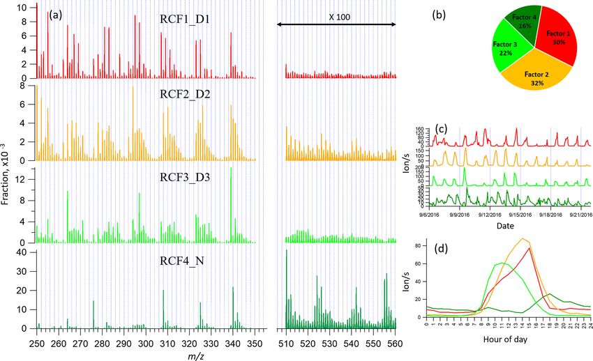
Iij 3.2 binPMF on Range 1 (250–300 Th)
σij = a × √ , (4)
ts
As has become routine (Zhang et al., 2011; Craven et al.,
where I is the signal intensity term, in unit of counts per sec- 2012), we first examined the mathematical parameters of our
ond (cps); ts stands for length of averaging in seconds, and solutions. From 2 to 10 factors, Q/Qexp decreased from 2.8
a is an empirical coefficient to compensate for unaccounted to 0.7 (Fig. S1 in Supplement), and after three factors the de-
uncertainties (Allan et al., 2003; Yan et al., 2016) and is 1.28 creasing trend was gradually slowing down and approaching
in our study as previously estimated from laboratory exper- 1, which is the ideal value for Q/Qexp as a diagnostic param-
iments (Yan et al., 2016). The σnoise term was estimated as eter. The unexplained variation showed a decline from 18 %
the median of the standard deviations from signals in the bins to 8 % from 2 to 10 factors.
in the region between nominal masses, where no physically In the two-factor results, two daytime factors were sepa-
meaningful signals are expected. rated, with peak time both at 14:00–15:00. One factor was
Atmos. Chem. Phys., 20, 5945–5961, 2020 https://doi.org/10.5194/acp-20-5945-2020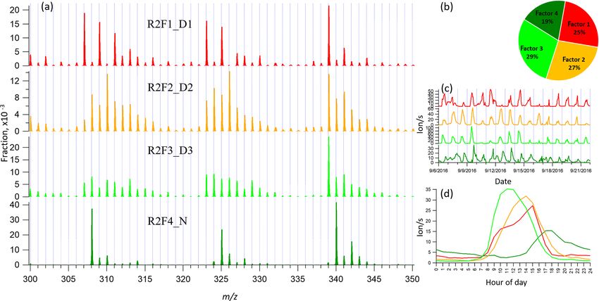
Y. Zhang et al.: Insights into atmospheric oxidation processes                                                                      5949

Figure 1. Example of mass spectrum with 1 h time resolution measured from a boreal forest environment during the IBAIRN campaign (at
18:00 LT, Finnish local time, UTC+2). The mass spectrum was divided into three parts, and three subranges were chosen from different parts
for further analysis in our study. The nitrate ion (62 Th) is included in the mass.

characterized by large signals at m/z 250, 255, 264, 281,              cycle but a distinct sawtooth shape. Factor 4 comes from a
283, 295, and 297 Th. The other factor was characterized               contamination of perfluorinated acids from the inlet’s auto-
by large signals at m/z 294, 250, 252, 264, 266, 268, and              mated zeroing every 3 h during the measurements (Zhang et
297 Th. In Hyytiälä, as reported in previous studies, odd              al., 2019). The zeroing periods have been removed from the
masses observed by the nitrate CI-APi-TOF are generally                dataset before binPMF analysis, but the contamination factor
linked to monoterpene-derived organonitrates during the day            was still resolved. This factor is discussed in more detail in
(Ehn et al., 2014; Yan et al., 2016). When the factor num-             Sect. 4.1 and 4.4.
ber increased to three, the two earlier daytime factors re-
mained similar to the previous result, while a new factor              3.3   binPMF on Range 2 (300–350 Th)
appeared with a distinct sawtooth shape in the diurnal cy-
cle. The main marker in the spectral profile was m/z 276 Th,           This range covers the monoterpene HOM monomer range,
with a clear negative mass defect. When one more factor was            and binPMF results have already been discussed by Zhang et
added, the previous three factors remained similar as in the           al. (2019) as a first example of the application of binPMF on
three-factor solution, and a new morning factor was resolved,          ambient data. Our input data here are slightly different. In the
with m/z 264 and 297 Th dominant in the mass spectral pro-             previous study, the 10 min automatic zeroing every 3 h was
file and a diurnal peak at 11:00.                                      not removed before averaging to 1 h time resolution, while
   As the factor number was increased, more daytime fac-               here we have removed these data. Overall, the results are sim-
tors were separated, with similar spectral profiles to existing        ilar as in our earlier study, and therefore the results are just
daytime factors and various peak times. No nighttime fac-              briefly summarized below for further comparison and discus-
tors were found in the analysis even when the factor number            sion in Sect. 4. Similar to Range 1, both the Q/Qexp (2.2 to
reached 10. We chose the four-factor result for further dis-           0.6) and unexplained variation (16 % to 8 %) declined with
cussion, and Fig. 2 shows the result of Range 1, with spectral         the increased factor number from 2 to 10.
profile, time series, diurnal cycle, and averaged factor contri-          When the factor number was two, one daytime factor and
bution during the campaign. As shown in Fig. 2d, factors 1–            one nighttime factor were separated, with diurnal peak times
3 are all daytime factors, while factor 4 has no clear diurnal         at 14:00 and 17:00, respectively. The nighttime factor was
                                                                       characterized by masses at 340, 308, and 325 Th (HOM

https://doi.org/10.5194/acp-20-5945-2020                                                 Atmos. Chem. Phys., 20, 5945–5961, 2020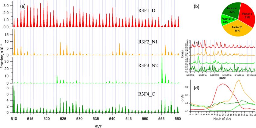
5950                                                                 Y. Zhang et al.: Insights into atmospheric oxidation processes

Figure 2. Four-factor result for Range 1 for (a) factor spectral profiles, (b) averaged factor contribution during the campaign, (c) time series,
and (d) diurnal trend. Details on the naming schemes for the factors are shown in Table 1.

monomers from monoterpene ozonolysis; Ehn et al., 2014)                    number (2–10). As can be seen from Fig. 1, data in Range
and remained stable throughout the factor evolution from 2                 3 had much lower signals compared to those of Range 1
to 10 factors. With the addition of more factors, no more                  and Range 2, explaining the higher unexplained variation for
nighttime factors got separated, while the daytime factor was              Range 3.
further separated and more daytime factors appeared, peak-                    In the two-factor result for Range 3, one daytime factor
ing at various times in the morning (10:00), at noon, or in                and one nighttime factor appeared, with diurnal peak times
the early afternoon (around 14:00 and 15:00). High contri-                 at noon and 18:00, respectively. The nighttime factor was
bution of m/z 339 Th can be found in all the daytime factor                characterized by ions at m/z 510, 524, 526, 542, 555, and
profiles. As the factor number reached six, a contamination                556 Th, while the daytime factor showed no dominant marker
factor appeared, characterized by large signals at m/z 339                 masses, yet with relatively high signals at m/z 516, 518,
and 324 Th, showing negative mass defects (Fig. S2). The                   and 520 Th. As the number of factors increased to three,
factor profile is nearly identical to the contamination factor             one factor with almost flat diurnal trend was separated, with
determined in Zhang et al. (2019), where the zeroing peri-                 dominant masses of 510, 529, and 558 Th. Most peaks in
ods were not removed, causing larger signals for the con-                  this factor had negative mass defects, and this factor was
taminants. In our dataset, where the zeroing periods were re-              again linked to a contamination factor. The four-factor re-
moved, no sawtooth pattern was discernible in the diurnal                  sult resolved another nighttime factor with a dominant peak
trend, yet it could still be separated even though it only con-            at m/z 555 Th and effectively zero contribution during day-
tributed 3 % to Range 2. More about the contamination fac-                 time. As the factor number was further increased, the new
tors from different ranges will be discussed in Sect. 4.4. We              factors seemed like splits from previous factors with simi-
chose to show the four-factor result below, to simplify the                lar spectral profiles. We therefore chose the four-factor result
later discussion and comparison. Figure 3 shows four-factor                also for Range 3 (results shown in Fig. 4) for further discus-
result of Range 2, with spectral profile, time series, diurnal             sion.
cycle, and averaged factor contribution during the campaign.
                                                                           3.5   binPMF on Range combined (250–350 and
3.4    binPMF on Range 3 (510–560 Th)                                            510–560 Th)

Range 3 represents mainly the monoterpene HOM dimers                       As a comparison to the previous three ranges, we conducted
(Ehn et al., 2014). Similar to Range 1 and Range 2, both                   the binPMF analysis on Range combined, which is the com-
the Q/Qexp (1.5 to 0.6) and unexplained variation (18 %                    bination of the three ranges. The results of this range are
to 15 %) showed decreasing trend with the increased factor                 fairly similar to those of Range 1 and Range 2, as could

Atmos. Chem. Phys., 20, 5945–5961, 2020                                                       https://doi.org/10.5194/acp-20-5945-2020
Y. Zhang et al.: Insights into atmospheric oxidation processes 5951 Figure 3. Four-factor result for Range 2 for (a) factor spectral profiles, (b) averaged factor contribution during the campaign, (c) time series, and (d) diurnal trend. Details on the naming schemes for the factors are shown in Table 1. Figure 4. Four-factor result for Range 3 for (a) factor spectral profiles, (b) averaged factor contribution during the campaign, (c) time series, and (d) diurnal trend. Details on the naming schemes for the factors are shown in Table 1. be expected since the signal intensities in these ranges were tor. In contrast, in the daytime factor, most masses were ob- much higher than in Range 3. As the number of factors served at odd masses and the fraction of signal in Range 3 increased (2–10), both the Q/Qexp (1.3 to 0.6) and unex- was much lower. During the day, photochemical reactions plained variation (16 % to 8 %) showed a decreasing trend. as well as potential emissions increase the concentration of In the two-factor result, one daytime factor and one night- NO, which serves as peroxy radical (RO2 ) terminator and of- time factor were separated. In the nighttime factor, most ten outcompetes RO2 cross reactions in which dimers can be masses were found at even masses, and the fraction of masses formed (Ehn et al., 2014). Thus, the production of dimers is in Range 3 was much higher than that in the daytime fac- suppressed during the day, yielding instead a larger fraction https://doi.org/10.5194/acp-20-5945-2020 Atmos. Chem. Phys., 20, 5945–5961, 2020
5952                                                                 Y. Zhang et al.: Insights into atmospheric oxidation processes

Figure 5. Four-factor result for Range combined for (a) factor spectral profiles, (b) averaged factor contribution during the campaign, (c) time
series, and (d) diurnal trend. Details on the naming schemes for the factors are shown in Table 1.

of organic nitrates, as has been shown also previously (Yan               resolved. The R2F4_N factor was characterized by signals at
et al., 2016).                                                            m/z 308 Th (C10 H14 O7 · NO−                                 −
                                                                                                        3 ), 325 Th (C10 H15 O8 · NO3 ),
                                                                                                        −
   With the increase in the number of factors, more daytime               and 340 Th (C10 H14 O9 · NO3 ), and they can be confirmed
factors were resolved with different peak times. When the                 as monoterpene ozonolysis products (Ehn et al., 2014; Yan
factor number reached seven, a clear sawtooth-shape diur-                 et al., 2016). With the increase in factor number to six, the
nal cycle occurred, i.e., the contamination factor caused by              contamination factor was separated also in this mass range.
the zeroing. As more factors were added, no further night-                In Range 3, one daytime factor, two nighttime factors, and a
time factors were separated, and only more daytime factors                contamination factor were separated. The first nighttime fac-
appeared. To simplify the discussion and inter-range com-                 tor (R3F2_N1) had large peaks at m/z 510 Th (C20 H32 O11 ·
parison, we also here chose the four-factor result for further            NO−                                      −
                                                                              3 ) and 556 Th (C20 H30 O14 · NO3 ), representing dimer
analysis. Figure 5 shows the four-factor result of Range com-             products that have been identified during chamber studies
bined, with spectral profile, time series, diurnal cycle, and             of monoterpene ozonolysis (Ehn et al., 2014). The molecule
averaged factor contribution during the campaign. The sig-                observed at m/z 510 Th has 32 H-atoms, suggesting that
nals in the range of 510–560 Th were enlarged 100-fold to be              one of the RO2 involved would have been initiated by OH,
visible.                                                                  which is formed during the ozonolysis of alkenes such as
                                                                          monoterpenes at nighttime (Atkinson et al., 1992; Paulson
                                                                          and Orlando, 1996). The other nighttime factor (R3F3_N2)
4   Discussion                                                            was dominated by ions at m/z 523 Th (C20 H31 O8 NO3 ·NO−     3)
                                                                          and 555 Th (C20 H31 O10 NO3 · NO−   3 ), representing nighttime
In Sect. 3, results by binPMF analysis were shown for Range
                                                                          monoterpene oxidation involving NO3 . As these dimers con-
1, Range 2, Range 3, and Range combined. In this section,
                                                                          tain only one N-atom, and 31 H-atoms, we can assume that
we discuss and compare the results from the different ranges.
                                                                          they are formed from reactions between an RO2 formed from
To simplify the inter-range comparison, we chose four-factor
                                                                          NO3 oxidation and another RO2 formed by ozone oxidation.
results for all four ranges, with the abbreviations shown in
                                                                          These results match well with the profiles in a previous study
Table 1. From Range 1, three daytime factors and a contami-
                                                                          by Yan et al. (2016). The results of Range combined are very
nations factor were separated. In Range 2, three daytime fac-
                                                                          similar to Range 2, with one nighttime factor and three day-
tors and one nighttime factor (abbreviated as R2F4_N) were

Atmos. Chem. Phys., 20, 5945–5961, 2020                                                       https://doi.org/10.5194/acp-20-5945-2020
Y. Zhang et al.: Insights into atmospheric oxidation processes 5953
time factors. The contamination factor was separated with combined (RCF1_D1) which did not show a clear correlation
increase in factor number to seven. with R3F1_D from Range 3 (Fig. 6e).
The second and third daytime factors in Range 1 and
4.1 Time series correlation Range 2, R1F2_D2, R1F3_D3, R2F2_D2, R2F3_D3, had
high correlations with R3F1_D in Range 3. Daytime factors
In Fig. 6, the upper panels show the time series correlations in Range combined (RCF2_D2 and RCF3_D3) also showed
among the first three ranges. As expected based on the results good correlation with R3F1_D in Range 3. However, if we
above, generally the daytime factors, and the two nighttime compare R3F1_D and the mass range of m/z 510–560 Th
monoterpene ozonolysis factors (R2F4_N and R3F2_N1), of the daytime factors in Range combined, just with a quick
correlated well. However, the contamination factors did not look, we can readily see the difference. The daytime factor
show a strong correlation between different ranges, even separated in Range 3 (R3F1_D) has no obvious markers in
though they are undoubtedly from the same source. More the profile. With the increase in factor number (up to 10 fac-
about the contamination factors will be discussed in Sect. 4.4. tors), no clearly new factors were separated in Range 3, but
The lower panels in Fig. 6 display the correlations between instead the previously separated factors were seen to split
into several factors. However, the spectral pattern in R3F1_D
the first three ranges and the Range combined, and they
clearly demonstrate that the results of Range combined are is different from that in the mass range of 510–560 Th in
mainly controlled by high signals from Range 1 and 2. More RCF2_D2. The factorization of Range combined was mainly
detailed aspects of the comparison between factors in differ- controlled by low masses due to their high signals. The sig-
ent ranges is given in the following sections. The good agree- nals at high masses were forced to be distributed according to
ments between factors from different subranges also help to the time series determined by small masses. Ultimately, this
verify the robustness of the solutions. will lead to failure in factor separation for this low-signal
range.
4.2 Daytime processes 4.2.2 Daytime dimer formation
4.2.1 Factor comparison Dimers are primarily produced during nighttime, due to NO
suppressing RO2 + RO2 reactions in daytime (Ehn et al.,
As mentioned above, with increasing number of factors, 2014; Yan et al., 2016). However, in this study, we found
more daytime factors will usually be resolved, reflecting the one clear daytime factor in Range 3 (R3F1_D, peak at local
complicated daytime photochemistry. The three daytime fac- time 12:00, UTC+2) by subrange analysis. With high load-
tors between Range 1 and Range 2 agreed with each other ings from even masses including 516, 518, 520, 528, and
quite well (Fig. 6a). However, R1F1_D1 and R2F1_D1 did 540 Th, this only daytime factor in dimer range correlated
not show strong correlations with the only daytime factor very well with two daytime factors in Range 1 and Range 2
in Range 3 (R3F1_D), while the other two daytime factors (R1F2_D2, R1F3_D3, R2F2_D2, R2F3_D3) (Fig. 6b and c).
in both Range 1 and Range 2, i.e., R1F2_D2, R1F3_D3, Table 2 includes the correlation matrix of all PMF and fac-
and R2F2_D2, R2F3_D3, correlated well with R3F1_D from tors and selected meteorological parameters. Strong correla-
Range 3. tion between R3F1_D with solar radiation was found, with
The first daytime factors from Range 1 and Range 2, R = 0.79 (Table 2). This may indicate involvement of OH
R1F1_D1 and R2F1_D1, were mainly characterized by odd oxidation in producing this factor.
masses: 255, 281, 283, 295, 297, 307, 309, 311, 323, 325, As previous studies have shown, dimers greatly facilitate
and 339 Th. The factors are dominated by organonitrates. Or- new particle formation (NPF) (Kirkby et al., 2016; Troestl et
ganic nitrate formation during daytime is generally associ- al., 2016; Lehtipalo et al., 2018), and this daytime dimer fac-
ated with the termination of RO2 radicals by NO. This ter- tor may represent a source of dimers that would impact the
mination step is mutually exclusive with the termination of initial stages of NPF in Hyytiälä. Mohr et al. (2017) reported
RO2 with other RO2 , which can lead to dimer formation. If a clear diel pattern of dimers (sum of about 60 dimeric com-
the NO concentration is the limiting factor for the forma- pounds of C16−20 H13−33 O6−9 ) during NPF events in 2013 in
tion of these factors, the low correlations between the NO- Hyytiälä, with minimum at night and maximum after noon,
terminated monomer factors and the dimer factors are to be and they estimated that these dimers can contribute ∼ 5 % of
expected. In contrast, if the other daytime factors mainly de- the mass of sub-60 nm particles. The link between the dimers
pend on oxidant and monoterpene concentrations, some cor- presented in that paper and those reported here will require
relation between those, and the daytime dimer factor, is to be further studies, as will the proper quantification of the dimer
expected, as shown in Fig. 6b and c. factor identified here.
All the spectral profiles resolved from Range combined
binPMF analysis inevitably contained mass contributions
from m/z 510 to 560 Th, even the daytime factor from Range
https://doi.org/10.5194/acp-20-5945-2020 Atmos. Chem. Phys., 20, 5945–5961, 20205954 Y. Zhang et al.: Insights into atmospheric oxidation processes
Table 1. Summary of PMF results for the different mass ranges.
Range Factor number Factor namea Dominant peaks Peak time
Range 1 (250–300 Th) 1 R1F1_D1 250, 255, 295, 297 15:00
2 R1F2_D2 250, 252, 294 15:00
3 R1F3_D3 264, 297 11:00
4 R1F4_C 276 –b
Range 2 (300–350 Th) 1 R2F1_D1 307, 309, 323, 325, 339 15:00
2 R2F2_D2 310, 326, 339 14:00
3 R2F3_D3 339 11:00
4 R2F4_N 308, 325, 340 18:00
Range 3 (510–560 Th) 1 R3F1_D 516, 518, 520, 528, 540 12:00
2 R3F2_N1 510, 524, 542, 556 18:00
3 R3F3_N2 523, 555 22:00
4 R3F4_C 510, 558 –b
Range combined (1, 2, 3) 1 RCF1_D1 250, 255, 295, 339 15:00
2 RCF2_D2 250, 252, 294, 339 14:00
3 RCF3_D3 264, 297, 339 11:00
4 RCF4_N 308, 340, 510, 524, 555, 556 18:00
a Factor name is defined with range name, factor number, and name. For example, Rx Fy represents factor y in range x . RC stands for Range
combined. For the factor name, D is short for daytime, N for nighttime, and C for contamination. b The contamination factor in Range 1
shows a sawtooth pattern, while Range 3 shows no diurnal pattern.
Figure 6. Time series correlations among Range 1, Range 2, Range 3 (a–c), and between the first three ranges and the Range combined (d–f).
The abbreviations for different factors are the same as in Table 1, with F for factor, D for daytime, N for nighttime, and C for contamination,
e.g. F1D1 for factor 1 daytime 1. The coefficient of determination, R 2 , is marked in each subplot by a number shown in the right upper
corners and by the blue colors, with stronger blue indicating higher R 2 .
Atmos. Chem. Phys., 20, 5945–5961, 2020 https://doi.org/10.5194/acp-20-5945-2020Y. Zhang et al.: Insights into atmospheric oxidation processes 5955
Table 2. Correlation between factors and meteorological parameters and gases.
4.3 Nighttime processes tween the spring dataset by Yan et al. (2016) and the au-
tumn dataset presented here is that nighttime concentrations
4.3.1 Factor comparison of HOMs were greatly reduced during our autumn campaign.
The cause may have been fairly frequent fog formation dur-
ing nights and also the fact that the concentration of ozone
Since high-mass dimers are more likely to form at night due
decreased nearly to zero during several nights (Zha et al.,
to photochemical production of NO in daytime, which in-
2018). It is also possible that the NO3 radical-related factor
hibits RO2 + RO2 reactions, Range 3 had the highest fraction
by Yan et al. (2016) is probably a mixture of NO3 and O3
of nighttime signals of all the subranges. While Range 3 pro-
radical chemistry, while the monomer may thus be attributed
duced two nighttime factors, Range 2 and Range combined
to the O3 part. Alternatively, the different conditions during
showed one, and Range 1 had no nighttime factor. The dif-
the two measurement periods, as well as seasonal difference
ference between the two results also indicates the advantage
in monoterpene mixtures (Hakola et al., 2012), caused varia-
of analyzing monomers and dimers separately.
tions in the oxidation pathways.
The two nighttime factors in Range 3 can be clearly iden-
tified as arising from ozonolysis (R3F2_N1) and a mix of
ozonolysis and NO3 oxidation (R3F2_N2) based on the mass 4.3.2 Dimers initiated by NO3 radicals
spectral profiles, as described above. The organonitrate at
m/z 555 Th, C20 H31 O10 NO3 · NO− 3 , is a typical marker for Previous studies show that NO3 oxidation of α-pinene, the
NO3 radical-initiated monoterpene chemistry (Yan et al., most abundant monoterpene in Hyytiälä (Hakola et al.,
2016). However, several interesting features become evident 2012), produces fairly little SOA mass (yields < 4 %), while
when comparing to the results of Range 2 and Range com- β-pinene shows yields of up to 53 % (Bonn and Moorgat,
bined. Firstly, only one nighttime factor (R2F4_N, RCF4_N) 2002; Nah et al., 2016). The NO3 + β-pinene reaction re-
was separated in each of these ranges, and that shows a clear sults in low-volatility organic nitrate compounds with car-
resemblance with ozonolysis of monoterpenes as measured boxylic acid, alcohol, and peroxide functional groups (Fry
in numerous studies, e.g., Ehn et al. (2012, 2014). Secondly, et al., 2014; Boyd et al., 2015), while the NO3 + α-pinene
the high correlation found in Fig. 6b between the ozonoly- reaction will typically lose the nitrate functional group and
sis factors (i.e., R2F4_N, R3F2_N1, RCF4_N) further sup- form oxidation products with high vapor pressures (Spittler
ports the assignment. However, factor R2F4_N is the only et al., 2006; Perraud et al., 2010). Most monoterpene-derived
nighttime factor in the monomer range, suggesting that NO3 HOMs, including monomers, are low-volatility molecules
radical chemistry of monoterpenes in Hyytiälä does not form (Peräkylä et al., 2020), and thus a low SOA yield indicates
substantial amounts of HOM monomers. The only way for a low HOM yield. Thus, while there are to our knowledge
the CI-APi-TOF to detect products of monoterpene-NO3 rad- no laboratory studies on HOM formation from NO3 oxida-
ical chemistry may thus be through the dimers, where one tion of α-pinene, a low yield can be expected based on SOA
highly oxygenated RO2 radical from ozonolysis reacts with studies.
a less oxygenated RO2 radical from NO3 oxidation. As discussed above, a dimer factor (R3F2_N2) was iden-
In the results by Yan et al. (2016) the combined UMR- tified as being a crossover between RO2 radicals initiated
PMF of monomers and dimers did yield a considerable by NO3 radicals and O3 . Figure 7 shows the time se-
amount of compounds in the monomer range also for the ries of this factor, as well as the products of [NO3 ]2 ×
NO3 radical chemistry factor. There may be several reasons [monoterpene]2 , [O3 ]2 × [monoterpene]2 , and [NO3 ] × [O3 ]
for this discrepancy. One major cause for differences be- × [monoterpene]2 . These products are used to mimic the for-
https://doi.org/10.5194/acp-20-5945-2020 Atmos. Chem. Phys., 20, 5945–5961, 20205956 Y. Zhang et al.: Insights into atmospheric oxidation processes Figure 7. Time series of the NO3 oxidation dimer factor (blue line) and the products of (a) [NO3 ]2 × [monoterpene]2 , (b) [O3 ]2 × [monoterpene]2 , and (c) [NO3 ] × [O3 ] × [monoterpene]2 , where [] represents concentration in units of pptv for NO3 radicals and monoter- pene and ppbv for O3 , while the scatter plots are shown as inserts, (d), (e), and (f), respectively. The scatter plots and correlation coefficients, R, are only calculated from nighttime data, which is selected based on solar radiation, to eliminate the influence from daytime oxidation processes. mation rates of the RO2 radicals reacting to form the dimers, surement (Liebmann et al., 2018), which in turn was some either from pure NO3 oxidation (Fig. 7a), pure O3 oxida- tens of meters away from the HOM measurements. Thus, this tion (Fig. 7b), or the mixed reaction between RO2 from the analysis should be considered qualitative only. two oxidants (Fig. 7c). The NO3 concentration was estimated The nitrate dimer factor (R3F2_N2) was dominated by the in Liebmann et al. (2018) for the same campaign. Monoter- organonitrate at m/z 555 Th, C20 H31 O10 NO3 · NO− 3 . How- penes were measured using a proton transfer reaction time- ever, unlike the pure ozonolysis dimer factor which had of-flight mass spectrometer (PTR-TOF-MS). More details on a corresponding monomer factor (R = 0.86 between factor measurement of NO3 proxy and monoterpene can be found R2F4_N and R3F2_N1), this NO3 -related dimer factor did in Liebmann et al. (2018). not have an equivalent monomer factor. This suggests that the As shown in Fig. 7, the time series of the dimer fac- NO3 oxidation of the monoterpene mixture in Hyytiälä does tor tracks those of [NO3 ]2 × [monoterpene]2 and [O3 ]2 × not by itself form much HOMs, but, in the presence of RO2 [monoterpene]2 reasonably well, but it shows the highest cor- from ozonolysis, the RO2 from NO3 oxidation can take part relation with the product of [NO3 ] × [O3 ] × [monoterpene]2 . in HOM dimer formation. This further implies that, unlike This further supports this dimer formation as a mixed pro- previous knowledge based on single-oxidant experiments in cess of ozonolysis and NO3 oxidation. The heterogeneity of chambers, NO3 oxidation may have a larger impact on SOA the monoterpene emissions in the forest, and the fact that no formation in the atmosphere where different oxidants exist dimer loss process is included, partly explains the relatively concurrently. This highlights the need for future laboratory low correlation coefficients. The sampling inlets for PTR- studies to consider systems with multiple oxidants during TOF were about 170 m away from the NO3 reactivity mea- monoterpene oxidation experiments to truly understand the Atmos. Chem. Phys., 20, 5945–5961, 2020 https://doi.org/10.5194/acp-20-5945-2020
Y. Zhang et al.: Insights into atmospheric oxidation processes                                                                 5957

role and contribution of different oxidants and NO3 in par-           4.5    Atmospheric insights
ticular.
                                                                      Based on the new data analysis technique, binPMF, applied
4.4   Fluorinated compounds                                           to subranges of mass spectra, we were able to separate two
                                                                      particularly intriguing atmospheric processes, the formation
During the campaign, an automated instrument zeroing ev-              of daytime dimers and dimer formation involving NO3 rad-
ery 3 h was conducted. While the zeroing successfully re-             icals, which otherwise could not have been identified in our
moved the low-volatility HOMs and H2 SO4 , the process also           study.
introduced contaminants into the inlet lines, e.g., perfluori-           With a diurnal peak around noontime, the daytime dimers
nated organic acids from Teflon tubing. Each zeroing pro-             identified in this study correlate very well with daytime
cess lasted for 10 min. In the data analysis, we removed all          factors in the monomer range. Strong correlation between
the 10 min zeroing periods, and averaged the data to 1 h time         this factor and solar radiation indicates the potential role of
resolution, but contaminants were still identified in all ranges      OH oxidation in the formation of daytime dimers. By now,
by binPMF. However, the correlation between contamination             very few studies have reported the observations of daytime
factors from different ranges is low (Fig. 6c).                       dimers. As dimers are shown to be able to take part in new
   To further investigate the low factor correlations of              particle formation (NPF) (Kirkby et al., 2016), this daytime
the same source, three fluorinated compounds with                     dimer may contribute to the early stages of NPF in the boreal
different volatilities, (CF2 )3 CO2 HF · NO−   3 (275.9748 Th),       forest.
(CF2 )5 C2 O4 H− (338.9721 Th), and (CF2 )6 CO2 HF · NO−         3       The second process identified in our study is the forma-
(425.9653 Th), were examined in fine time resolution, i.e.,           tion of dimers that are a crossover between NO3 and O3
1 min. The time series and 3 h cycle of the three fluorinated         oxidation. Such dimers have been identified before (Yan et
compounds were shown in Figs. S3 and S4. The correlation              al., 2016). However, we were not able to identify corre-
coefficients dropped greatly before and after the zero period         sponding HOM monomer compounds. This finding indicates
was removed: from 0.9 to 0.3 for R 2 between m/z 276 and              that while NO3 oxidation of the monoterpenes in Hyytiälä
339 Th and 0.8 to 0.1 between m/z 276 and 426 Th (Fig. S5a,           may not undergo autoxidation to form HOMs by themselves,
b). A similar effect is also found with the 1 h averaged data         they can contribute to HOM dimers when the NO3 -derived
(Fig. S5c, d). It is evident that the three fluorinated com-          RO2 reacts with highly oxygenated RO2 from other oxidants.
pounds were from the same source (zeroing process), but due           Multi-oxidant systems should be taken into consideration in
to their different volatilities, they were lost at different rates.   future experimental studies on monoterpene oxidation pro-
This, in turn, means that the spectral signature of this source       cesses.
will change as a function of time, at odds with one of the
basic assumptions of PMF.
   The analysis of the fluorinated compounds in our system            5     Conclusions
was here merely used as an example to show that volatil-
ity can impact source profiles over time. In Fig. S5, it can          The recent developments in the field of mass spectrometry,
be clearly seen that the profile of Range combined is noisier         combined with factor analysis techniques such as PMF, have
than that of Range 3, probably due to the varied fractional           greatly improved our understanding of complicated atmo-
contributions of contamination compounds to the profile. In           spheric processes and sources. In this study, we applied the
ambient data, products from different sources can have un-            new binPMF approach (Zhang et al., 2019) to separate sub-
dergone atmospheric processing, altering the product distri-          ranges of mass spectra measured using a chemical ioniza-
bution. This analysis highlighted the importance of differ-           tion mass spectrometer in the Finnish boreal forest. By using
ences in the sink terms due to different volatilities of the          this method, we were able to identify a daytime dimer fac-
products. This may be an important issue for gas-phase mass           tor, presumably initiated by OH/O3 oxidation of monoter-
spectrometry analysis, potentially underestimated by many             penes, forming from RO2 + RO2 reactions despite compe-
PMF users, as it is likely only a minor issue for aerosol data,       tition from daytime NO. This compound group, showing a
for which PMF has been applied much more routinely. If fail-          diurnal peak around noon, may contribute to new particle
ing to achieve physically meaningful factors using PMF on             formation at the site. In addition, we successfully separated
gas-phase mass spectra, our recommendation is to try apply-           NO3 -related dimers which would not have been identified
ing PMF to subranges of the spectrum, where intermediate-             from this dataset without utilizing the different subranges.
volatility organic compounds (IVOCs), semivolatile organic            The NO3 -related factor was consistent with earlier obser-
compounds (SVOCs), and (extremely) low volatility organic             vations (Yan et al., 2016), with the exception that we did
compounds ((E)LVOCs) could be analyzed separately.                    not observe any corresponding monomer factor. This may
                                                                      be explained by the observed nitrate-containing dimers being
                                                                      formed from two RO2 radicals, where one is initiated by ox-
                                                                      idation by O3 and the other by NO3 . If the NO3 -derived RO2

https://doi.org/10.5194/acp-20-5945-2020                                               Atmos. Chem. Phys., 20, 5945–5961, 2020
5958 Y. Zhang et al.: Insights into atmospheric oxidation processes
radicals are not able to form HOMs by themselves, there will Financial support. This research has been supported by the Euro-
not be any related monomers observed. To validate this hy- pean Research Council (grant no. 638703-COALA), the Academy
pothesis, future laboratory experiments that target more com- of Finland (grant nos. 317380 and 320094), and the Swiss National
plex oxidation systems will be useful in order to understand Science postdoc mobility grant (grant no. P2EZP2_181599).
the role of NO3 oxidation in SOA formation under different
Open access funding provided by Helsinki University Library.
atmospheric conditions.
Apart from these two major findings, we also found sev-
eral other benefits of applying PMF on separate subranges
Review statement. This paper was edited by James Allan and re-
of the mass spectra. First, different compounds from the
viewed by two anonymous referees.
same source can have variable loss rates due to differences
in volatilities. This leads to increased difficulty for PMF to
separate this source, but if the PMF analysis is run sepa-
rately on lighter masses (with higher volatility) and heavier References
masses (with lower volatility), the source may become easier
to distinguish. Secondly, chemistry or sources contributing Allan, J. D., Jimenez, J. L., Williams, P. I., Alfarra, M. R., Bower,
K. N., Jayne, J. T., Coe, H., and Worsnop, D. R.: Quantitative
only to one particular mass range, e.g., dimers, can be better
sampling using an Aerodyne aerosol mass spectrometer 1. Tech-
separated. Thirdly, mass ranges with small, but informative, niques of data interpretation and error analysis, J. Geophys. Res.-
signals can be more accurately assigned as their contribu- Atmos., 108, https://doi.org/10.1029/2002JD002358, 2003.
tion becomes larger than if the entire mass range was ana- Atkinson, R., Aschmann, S. M., Arey, J., and Shorees, B.: For-
lyzed at once. Finally, running PMF on separate mass ranges mation of OH radicals in the gas phase reactions of O3
also allows for comparing the factors between the different with a series of terpenes, J. Geophys. Res., 97, 6065–6073,
ranges, helping to verify the results. In summary, while we https://doi.org/10.1029/92jd00062, 1992.
do not suggest that this type of subrange analysis should al- Berndt, T., Mentler, B., Scholz, W., Fischer, L., Herrmann,
ways be utilized, we recommend other analysts of gas-phase H., Kulmala, M., and Hansel, A.: Accretion Product For-
mass spectrometer data to test this approach in order to see mation from Ozonolysis and OH Radical Reaction of α-
whether additional useful information can be obtained. In Pinene: Mechanistic Insight and the Influence of Isoprene
and Ethylene, Environ. Sci. Technol., 52, 11069–11077,
our dataset, this method was crucial for identifying different
https://doi.org/10.1021/acs.est.8b02210, 2018a.
types of dimers and dimer formation pathways, which are of
Berndt, T., Scholz, W., Mentler, B., Fischer, L., Herrmann, H., Kul-
great importance for the formation of both new particles and mala, M., and Hansel, A.: Accretion Product Formation from
SOA. Self- and Cross-Reactions of RO2 Radicals in the Atmosphere,
Angewandte Chemie International Edition in English, 57, 3820–
3824, https://doi.org/10.1002/anie.201710989, 2018b.
Data availability. The data used in this study are available from Bertram, T. H., Kimmel, J. R., Crisp, T. A., Ryder, O. S., Yatavelli,
the first author upon request: please contact Yanjun Zhang (yan- R. L. N., Thornton, J. A., Cubison, M. J., Gonin, M., and
jun.zhang@helsinki.fi). Worsnop, D. R.: A field-deployable, chemical ionization time-
of-flight mass spectrometer, Atmos. Meas. Tech., 4, 1471–1479,
https://doi.org/10.5194/amt-4-1471-2011, 2011.
Supplement. The supplement related to this article is available on- Bianchi, F., Kurtén, T., Riva, M., Mohr, C., Rissanen, M. P., Roldin,
line at: https://doi.org/10.5194/acp-20-5945-2020-supplement. P., Berndt, T., Crounse, J. D., Wennberg, P. O., Mentel, T. F.,
Wildt, J., Junninen, H., Jokinen, T., Kulmala, M., Worsnop, D.
R., Thornton, J. A., Donahue, N., Kjaergaard, H. G., and Ehn,
Author contributions. ME and YZ designed the study. QZ and MR M.: Highly Oxygenated Organic Molecules (HOM) from Gas-
collected the data; data analysis and article writing were done by Phase Autoxidation Involving Peroxy Radicals: A Key Con-
YZ. All coauthors discussed the results and commented on the arti- tributor to Atmospheric Aerosol, Chem. Rev., 119, 3472–3509,
cle. https://doi.org/10.1021/acs.chemrev.8b00395, 2019.
Bonn, B. and Moorgat, G. K.: New particle formation during
a- and b-pinene oxidation by O3 , OH and NO3 , and the in-
fluence of water vapour: particle size distribution studies, At-
Competing interests. The authors declare that they have no conflict
mos. Chem. Phys., 2, 183–196, https://doi.org/10.5194/acp-2-
of interest.
183-2002, 2002.
Boyd, C. M., Sanchez, J., Xu, L., Eugene, A. J., Nah, T., Tuet, W.
Y., Guzman, M. I., and Ng, N. L.: Secondary organic aerosol
Acknowledgements. We thank the tofTools team for providing tools formation from the β-pinene+NO3 system: effect of humidity
for mass spectrometry data analysis. The personnel of the Hyytiälä and peroxy radical fate, Atmos. Chem. Phys., 15, 7497–7522,
forestry field station are acknowledged for help during field mea- https://doi.org/10.5194/acp-15-7497-2015, 2015.
surements. Canagaratna, M., Jayne, J., Jimenez, J., Allan, J., Alfarra, M.,
Zhang, Q., Onasch, T., Drewnick, F., Coe, H., and Middle-
Atmos. Chem. Phys., 20, 5945–5961, 2020 https://doi.org/10.5194/acp-20-5945-2020You can also read