Model-free estimation of available power using deep learning - WES
←
→
Page content transcription
If your browser does not render page correctly, please read the page content below
Wind Energ. Sci., 6, 111–129, 2021
https://doi.org/10.5194/wes-6-111-2021
© Author(s) 2021. This work is distributed under
the Creative Commons Attribution 4.0 License.

                             Model-free estimation of available
                                power using deep learning
                     Tuhfe Göçmen, Albert Meseguer Urbán, Jaime Liew, and Alan Wai Hou Lio
                           Department of Wind Energy, DTU, Technical University of Denmark,
                                    Frederiksborgvej 399, 4000 Roskilde, Denmark
                                     Correspondence: Tuhfe Göçmen (tuhf@dtu.dk)

                                Received: 28 October 2019 – Discussion started: 7 November 2019
                         Revised: 29 July 2020 – Accepted: 8 December 2020 – Published: 18 January 2021

       Abstract. In order to assess the level of power reserves during down-regulation, the available power of a
       wind turbine needs to be estimated. The current practice in available power estimation is heavily dependent
       on the pre-defined performance parameters of the turbine and the curtailment strategy followed. This paper
       proposes a single-input model-free approach dynamic estimation of the available power using recurrent neural
       networks. Accordingly, it combines wind turbine control considerations and modern forecasting methodologies
       for a model-free, single-input estimation of available power. It enables a robust real-time implementation of
       dynamic delta control, as well as higher-accuracy provision of the reserves to the system operators.
          The model-free approach requires only 1 Hz wind speed measurements as input and estimates 1 Hz available
       power as output. The neural network is trained, tested and validated using the DTU 10 MW reference wind
       turbine HAWC2 model under realistic atmospheric conditions. The unsteady patterns in the turbulent flow are
       represented via long short-term memory (LSTM) neurons which are trained during a period of normal operation.
       The adaptability of the network to changing inflow conditions is ensured via transfer learning, where the last
       LSTM layer is updated using new measurements. It is seen that the sensitivity of the networks to changing
       wind speed is much higher than that of turbulence, and the updates are to be implemented solely based on the
       altering inflow velocity. The validation of the trained LSTM networks on time series with 7, 9 and 11 m s−1
       mean wind speeds demonstrates high accuracy (less than 1 % bias) and capability of transfer-learning online.
       Including highly turbulent inflow cases, the networks have shown to comply with the most recent grid codes,
       which require the quality of the available power estimations to be evaluated with high accuracy (less than 3.3 %
       standard deviation of the error around zero bias) at 1 min intervals.

1   Introduction                                                     The curtailment of wind turbines can be implemented both
                                                                  as balance control, where the turbine power output is reduced
As the share of wind energy increases in power systems            to a constant value, and as delta control, where the output is
around the world, new challenges regarding the control and        reduced by a certain percentage of the available power (Attya
operations of wind power plants are encountered. In order to      et al., 2018; Fleming et al., 2016; Hansen et al., 2006). Ad-
maintain power system stability, transmission system opera-       ditionally, the active power reduction for both strategies can
tors (TSOs) are developing new grid codes requiring contri-       be achieved by adjusting the rotor blade pitch angles and/or
butions not only from conventional generators, but also from      operating at a sub-optimal rotor speed compared to the maxi-
wind power plants, globally. In this context, here we focus       mum energy capture value (Wilches-Bernal et al., 2016). Al-
on the active power contribution of wind turbines to provide      though modern turbines are capable of implementing both
frequency support and power reserves via down-regulation          balance and delta control, due to the uncertainties in the esti-
(also referred to as curtailment, de-rating or de-loading).       mated available power (Göçmen et al., 2016; Göçmen and
                                                                  Giebel, 2018; Göçmen et al., 2019; Pinson, 2006; Pinson

Published by Copernicus Publications on behalf of the European Academy of Wind Energy e.V.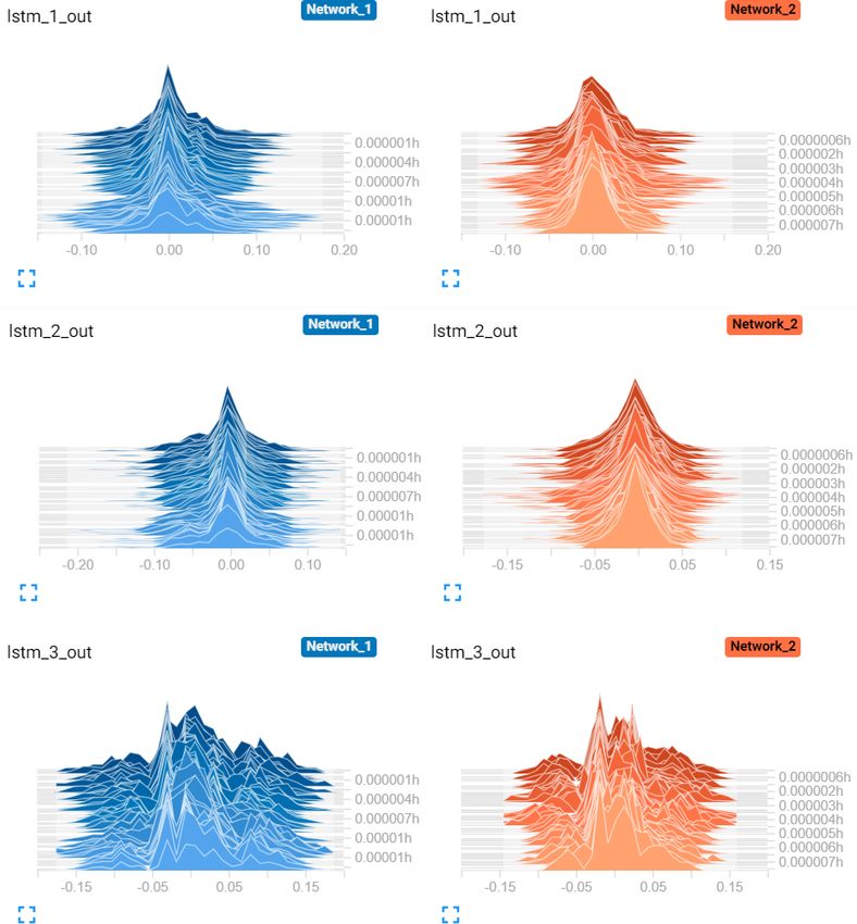
112                                           T. Göçmen et al.: Model-free estimation of available power using deep learning

et al., 2007), balance control is the preferred industrial appli-   tion, which is widely adopted in the wind turbine industry as
cation as its set point is independent of the available power       well as the wind research community (e.g. van der Hooft and
(Kristoffersen, 2005). The amount of power reserves how-            van Engelen, 2004; Göçmen et al., 2014). More details on the
ever, which is defined as the difference between the available      approach are provided in Sect. 2. Ma et al. (1995) demon-
and the produced power under curtailed operation, does de-          strate that directly mapping the static relation does not give
pend on the available power in the wind for both delta and          satisfactory performance and concludes that the inclusion of
balance control. This is particularly critical for compensa-        dynamic models can significantly improve the wind speed
tion schemes under mandatory down-regulation, as well as            estimate. Thus, an increasing number of studies (e.g. Øster-
(existing and expected) flexible balancing market structures,       gaard et al., 2007; Meng et al., 2016) began to utilize ob-
where the reserve power is traded at different timescales de-       server theory, in particular, Kalman filtering. For example,
pending on the regional balancing market schemes (Chinmoy           in Østergaard et al. (2007), the aerodynamic torque is con-
et al., 2019).                                                      sidered a system disturbance state, and it is estimated by the
   Generally, trading in the electricity markets is performed       use of an observer-based system on a simple drivetrain model
in advance with a given forecast horizon. Depending on the          with pre-defined dynamics for the aerodynamic torque. Sub-
bidding structure, the available power production of an as-         sequently, the calculation of the wind speed is done by inver-
set is to be predicted sometimes as shortly as 5 min ahead          sion of the static mapping between the aerodynamic torque
(e.g. Rana and Koprinska, 2016). The forecasting tools can          and wind speed. One of the drawbacks of searching through
be based on physical or statistical modelling, as well as           the static relation, to find the wind speed estimate, is its com-
the combination of both. Many perform post-processing via           putational cost, where a Newton–Raphson method is often
model output statistics to reduce the remaining error. Some         employed to find the corresponding wind speed given the
approaches focus on the best possible estimate of the local         turbine measurement on a discrete power coefficient CP of
wind speed while some directly extract the wind power gen-          surface. On the other hand, some methods do not require the
eration potential. Statistical models use explanatory variables     use of iterative gradient methods, for example, by consid-
and historical/online information (measurements, log-data,          ering the wind speed directly as a state to the system, and
etc.), generally implementing recursive techniques, such as         such a wind state can be estimated via an observer Kalman
recursive least-squares or artificial neural networks (or deep      filter. In Selvam (2007), the wind dynamics are modelled as
learning) (Wang et al., 2016). In fact, forecasting is the field    a random walk and augmented with a linear turbine model
with the most deep-learning (and broadly artificial intelli-        including a simple drivetrain and tower dynamic model. A
gence) applications in wind energy, e.g. Ghaderi et al. (2017),     linear Kalman filter is then employed to estimate the wind
Chen et al. (2018) and Mujeeb et al. (2019). For a recent re-       speed for feed-forward control purpose. Similar techniques
view on deep-learning-based wind speed forecasting for sev-         have also been utilized in Stol and Balas (2003) and Simley
eral forecast horizons, see Bali et al. (2019). However, while      and Pao (2016). A study by Knudsen et al. (2011) employed
forecasting the available power, the operational status and         a non-linear turbine model including simple drivetrain, tower
potential effects of control scenarios are often overlooked,        and wind speed dynamics where the effective wind speed is
especially for higher (than e.g. 5 min) frequencies at a single     estimated by an extended Kalman filter. Similar methods are
turbine level.                                                      also reported in Henriksen et al. (2012), where the dynamic
   For the operational considerations and higher-frequency          inflow model is included. Besides the Kalman-filter-based
system stability issues, the timescales considered in the           approaches, some studies (Ortega et al., 2011, 2013) used a
market-based forecasting are already long-term ahead. In or-        more advanced state estimation technique of immersion and
der for the balancing responsible parties to be compensated         invariance to construct a wind speed estimation with proof
for during mandatory down-regulation by the TSOs, wind              of global convergence under certain assumptions. For more
power plants are expected to provide information regarding          details and further information on wind speed estimation, see
their power production on much shorter timescales. As stated        Soltani et al. (2013) and references therein.
in the recent grid requirements in Germany (50Hertz, Am-                The state-of-the-art available power estimation is highly
prion, Tennet, TransnetBW, 2016), the available power is            dependent on the considered turbine models, as well as the
to be calculated for 60 s intervals for down-regulated wind         operation strategy for curtailment. More specifically, the ma-
farms. Additionally, the 1 min standard deviation of the per-       jority of the methods rely on the pre-calculated power co-
centage error of the available power is required to be less than    efficient, CP , or the certified nominal power curve to con-
±3.3 % (after the pilot phase). The enforced regulations are        vert (rotor-effective) wind speed to (available) power. How-
difficult to comply with and are subject to penalty if not met.     ever, the varying wind speed and turbulence levels activate
   The current practice in available power estimation is to as-     different dynamics within the turbine structure and cause
sess the incoming wind speed to derive the possible power           different control responses (Murcia et al., 2018). In addi-
output of the turbine via optimum performance curve. One            tion, temporally and spatially local characteristics of the flow
of the most common approaches to approximate the (effec-            (e.g. humidity, temperature) and the condition of the turbine
tive) wind speed is by solving the static wind power equa-          (e.g. blade erosion, dust, component wear or failure) highly

Wind Energ. Sci., 6, 111–129, 2021                                                      https://doi.org/10.5194/wes-6-111-2021
T. Göçmen et al.: Model-free estimation of available power using deep learning                                                    113

                                                                  sults are publicly available1 . First, the sensitivity of the state-
                                                                  of-the-art available power predictions to the curtailment op-
                                                                  eration strategy is briefly discussed and quantified in Sect. 2.
                                                                  To address the issue, a detailed analysis of LSTM neural net-
                                                                  works and the potential of transfer learning to adapt to chang-
                                                                  ing inflow conditions is presented throughout Sect. 3. This
                                                                  research focus is highly important for the individual turbine
                                                                  control and its role in the power system stability, as well as
                                                                  the business case of wind energy in the existing and upcom-
                                                                  ing market scenarios.
Figure 1. Flow diagram of the model-free approach to estimating
available power.                                                  2   Wind speed to power via turbine model

                                                                  As stated earlier, current methods for estimating available
                                                                  power typically make use of pre-defined power curves or
                                                                  power coefficient calculations. Here in this section, we dis-
affect the CP and the power curve behaviour. Therefore, these     cuss the assessment of wind speed and the sensitivity of the
generally deterministic approaches fail to represent the de-      model-dependent approaches to the implemented curtailment
tailed dynamics required to produce high-frequency available      strategy.
power signal accurately (Jin and Tian, 2010), and they are an        Point measurements of the wind speed using, for example,
important source of uncertainty (Lange, 2005). In order to        cup or sonic anemometers, are often unreliable at estimating
tackle the inadequacy of the turbine models to fully repre-       the potential power production of a wind turbine as the spa-
sent the dynamic power output of a turbine under turbulent        tial variations in the wind field are not captured. For example,
inflow, a model-free approach to transfer the wind speed to       a naive approach at estimating available power is
power is a strong alternative.
                                                                                1
   Therefore in this study, the aim is to consider the wind       Pavail (U ) = ρπ R 2 CP U 3 ,                               (1)
turbine generator (WTG) control and modern forecasting                          2
methodologies for a model-free, single-input estimation of        where the air density, ρ; rotor radius, R; and power coef-
available power. It enables a robust real-time implementa-        ficient, CP , are assumed to be constant with variable (effec-
tion of dynamic delta control, as well as the provision of the    tive) wind speed, U . Equation (1) presents a number of weak-
reserves to the system level within the frame of (strictest)      nesses, namely the inability to capture the dynamic response
European grid regulations. In the model-free estimation of        of the wind turbine to changing wind speeds, or the spatial
available power, the unsteady patterns in the turbulent flow      variations in the wind field. For this reason, the rotor effec-
are represented via long short-term memory (LSTM) neu-            tive wind speed, which is defined as the spatial average wind
rons (Hochreiter and Schmidhuber, 1997), which is a special       speed over the rotor plane, is preferred in terms of power
building unit for recurrent neural networks (RNNs). The pro-      estimation. Although there are numerous methods for esti-
posed method for integrating an LSTM network in a curtail-        mating rotor effective wind speed, the majority of methods
ment strategy is outlined in Fig. 1. During a period of nor-      use operating data of the wind turbine to create the estimate
mal operation of a WTG, wind speed and power output time          (Jena and Rajendran, 2015). A simple strategy is to estimate
series data are collected for at least an hour to establish a     the wind speed for a given power output using a polynomial
training dataset. Next, the network is trained on the collected   fit (Thiringer and Petersson, 2005). This method can be ex-
data which, depending on the available processing power, can      tended by including the rotor speed and blade pitch angle in
be performed within seconds. Accordingly, the wind turbine        conjunction with a CP look-up table to infer the wind speed
operator can announce its participation in the reserve market     as shown in Bhowmik et al. (1998). For derated operation,
online or ahead of time with the intention of performing delta    these methods are problematic as the dependency between
or balance control for curtailment. Down-regulation is then       the wind speed and a turbine’s operating points varies based
performed using the LSTM predictor which provides the set         on the desired level of down-regulation. The use of a prede-
point based on the available power. The model-free estima-        fined CP curve to estimate available power therefore becomes
tion approach can be rapidly retrained with newly collected       unreliable. However, state space approaches where the con-
data using transfer learning, where the last LSTM layer of        vergence of the wind estimation error is analysed systemati-
the network is updated using the new information.                 cally can potentially respond to that problem.
   The synthetic time series used in this study is generated          1 The      generated     time      series     can     be      ac-
using the DTU 10 MW reference wind turbine (Bak et al.,           cessed           here:         https://gitlab.windenergy.dtu.dk/tuhf/
2013) with the aeroelastic code HAWC2 (Bak et al., 2012)          deep-learning-for-available-power-estimation/tree/master/data
under realistic atmospheric conditions, and the simulation re-    (last access: 29 July 2020).

https://doi.org/10.5194/wes-6-111-2021                                                      Wind Energ. Sci., 6, 111–129, 2021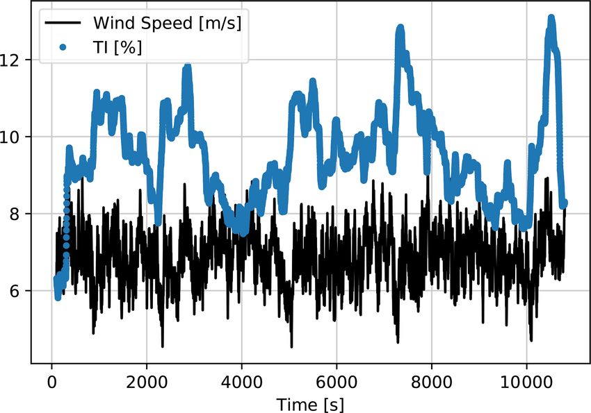
114 T. Göçmen et al.: Model-free estimation of available power using deep learning
∂h xk−
There are several benefits of formulating a wind speed es- Pk+ = (I − Lk Hk ) Pk− , Hk := (3b)
timation as a system state estimation problem compared to ∂x
methods that use static relation mapping the power or aero-
Here Lk ∈ Rnx ×ny is the filter gain and it is computed as fol-
dynamic torque to wind speed. For example, a substantial
lows:
body of mature and sophisticated state estimation theory can
immediately be brought to bear upon the design of the wind Lk = Pk− HkT (Hk Pk− HkT + Rk )−1 , (3c)
estimator. Moreover, in an observer design where the wind
speed is considered a system state, the use of slow gradi- where Qk ∈ Rnx ×nx and Rk ∈ Rnu ×nu denote the co-variance
ent methods for solving the static relations can be avoided, matrices of the process and measurement noises, respec-
tively, that can be computed as Qk = E[wn,k wn,k T ], R =
resulting in better computational speed and a smooth wind k
speed estimate. T ]T . The process co-variance Q is chosen by ap-
E[vn,k vn,k k
Typically, to formulate a state estimation problem, a sim- proximating the variance of the modelling error and the typi-
plified model of the non-linear dynamics is required that cal wind speed. In this work, there is no measurement noise;
needs to capture the key dynamics of the turbine. For brevity, thus, the measurement co-variance Rk is chosen as a small
a widely used non-linear turbine system model is employed, value.
including the dynamics of rotor drivetrain, tower and wind One of the weaknesses of the EKF filtering approach is
speed (see Knudsen et al., 2011; Lio et al., 2019): being a model-based method that requires a relatively accu-
rate model of the turbine. Besides, the choice of the model,
xk+1 = f (x k , uk ) + wn,k , (2a) operating conditions and sensor locations also strongly af-
yk = h (x k , uk ) + vn,k , (2b) fects the EKF-based estimator performance (Lio et al., 2019).
Some studies (e.g. Lio et al., 2018) showed that down-
where x k = [ωk , ẋfa,k , xfa,k , vk ]T ∈ Rnx is the system state regulation can be achieved by either modifying the gener-
vector at the sample time k ∈ Z containing the rotor speed, ator torque solely or the combinations of rotor speed and
fore-aft velocity and displacement of the tower-top and torque. The constant and maximum rotation (Const- and
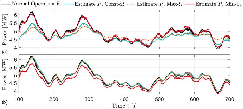
ambient wind speed, whilst the system input uk = [τg,k , Max-) strategies perform down-regulation by setting the
θk ]T ∈ Rnu contains the generator torque and pitch angle, rotor speed to a pre-determined or maximum value whilst the
and yk = [ωk , ẋfa,k , xfa,k ]T ∈ Rny denotes the system out- Min-Ct methods operate the turbine at a minimum thrust co-
put. The state transition and output functions are denoted efficient in down-regulation. The performances of the EKF
as f : Rnx × Rnu → Rnx , h : Rnx × Rnu → Rny . The Gaus- based upon these operations are shown in Fig. 2. The sim-
sian process noise wn,k ∈ Rnx represents the modelling errors ulations are based on the DTU 10 MW reference wind tur-
whilst the Gaussian measurement noise vn,k ∈ Rny represents bine HAWC2 model (Bak et al., 2012) under 9 m s−1 mean
the sensor noise and modelling error of the sensor dynamics. wind speed and 10 % mean turbulence intensity over 700 s.
Since the turbine model is a nonlinear model (Eq. 2a), The turbines are commanded to operate at 40 % and 80 % of
an extended Kalman filter (EKF) is employed to compute the rated power. One clear message from Fig. 2 is that the
estimates of the wind turbine state. A Kalman filter is a performance of the EKF-based wind estimator is highly sub-
computationally efficient and recursive algorithm that pro- jected to the turbine operating conditions; for example, the
vides the optimal state estimates x̂k ∈ Rnx by minimizing the performances were similar for strategies operating at 80 %
mean square state error or the state error covariance matrix but the Max- performed the worst at 40 % down-regulation.
Pk := E[(xk − x̂k )(xk − x̂k )T ]. Kalman filtering approaches Similarly, Min-Ct shows the best agreement with the avail-
have been effectively employed in many examples of wind able power for 40 % down-regulation whereas it performs
energy (e.g. Ritter et al., 2018; Lio, 2018; Annoni et al., the worst for 80 % curtailment. Therefore, Fig. 2 indicates
2018). Typically, in EKF, the estimate of the state x̂k is com- no clear trend and high sensitivity of model-based methods
puted in two-step processes: prediction and measurement up- to the control scenario.
date. The superscripts xk+ and xk− are denoted as the vari- It should be noted that the sensitivity observed in the syn-
able x at sample time k after the measurement update and thetic time series in Fig. 2 is expected to grow under the
before the measurement update, respectively. The hat nota- field conditions. This is due to the fact that the manufacturer-
tion x̂ denotes the estimate of x. calibrated power coefficients cannot account for variability
influenced by local conditions (Bandi and Apt, 2016). Ad-
Prediction : ditionally, the resulting uncertainty of the CP -dependent ap-
x̂k− = f x̂k−1
+
, uk , Pk− = Fk Pk−1
+
FkT + Qk
proaches is likely to also be amplified due to the lack of de-
+ tailed information regarding the pre-defined CP and imple-
∂f x̂k−1
Fk := (3a) mented operation strategy for curtailment caused by the lim-
∂x ited access to the controller in practice. To avoid the depen-
Measurement update : dency on operating point estimations of available power, the
ŷ = h x̂k− , uk , x̂k+ = x̂k− + Lk yk − ŷk
use of wind speed measurements is revisited with the state-
Wind Energ. Sci., 6, 111–129, 2021 https://doi.org/10.5194/wes-6-111-2021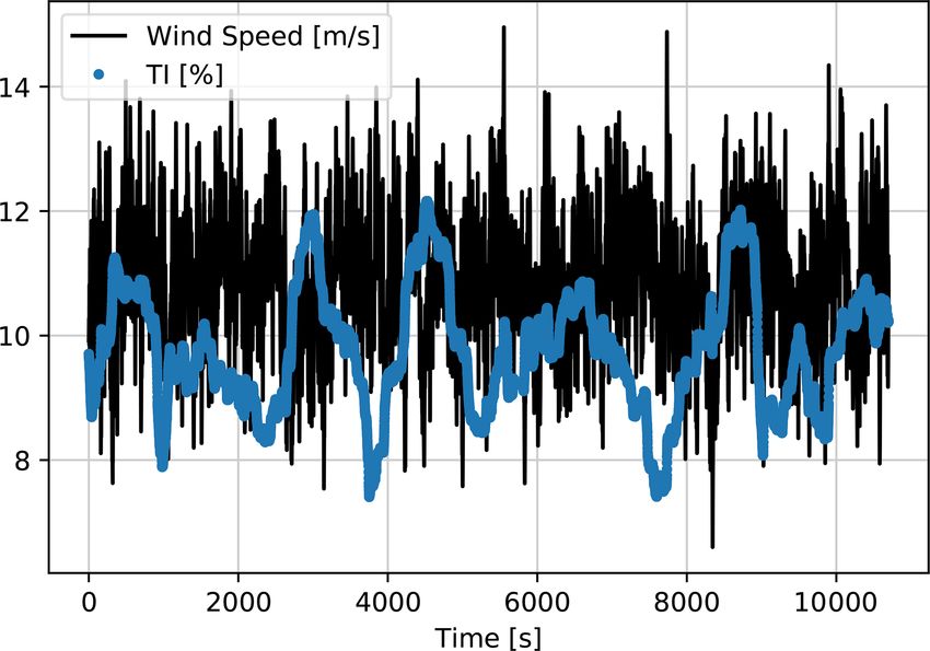
T. Göçmen et al.: Model-free estimation of available power using deep learning                                                      115

Figure 2. Time series of normal power Pn and available power estimation P̂ based upon various down-regulation strategies. (a) and (b) in-
dicate the estimation based on measurements of turbines operating at 40 % and 80 % of the rated power, respectively.

of-the-art deep-learning architecture in the next section. The         the LSTM algorithm. LSTM architecture is a special type of
performance of this model-free approach is then compared               RNN, which is shown to perform faster and better for highly
with the presented wind speed observer, also for the scenario          fluctuating time series than many other RNN architectures.
with limited CP information during down-regulation.                    An LSTM neuron is illustrated in Fig. 3, where there is no di-
                                                                       rect connection between the input it and the output ot gates.
                                                                       All the information flows through the cell state ct , which is
3   Neural networks for available power set point
                                                                       the actual memory of the LSTM neuron, and it is regulated by
For a more robust operation and delta control, the bias and            the forget gate ft to avoid indefinite growth and eventual net-
the uncertainties, which partly originate from the natural             work break down (Gers et al., 2000). Through the calibrated
variability of the flow and turbulence and partly due to the un-       weights, ft decides how much of the previous cell state(s) is
certainty associated with the turbine models, i.e. CP surfaces,        preserved, following Eq. (4).
should be reduced. The former is investigated through a state-         ft = σ Wfi xt0 + Wfo ht1 + bf ,

                                                                                                                                   (4)
space update via Kalman filters in Sect. 2. Here, we imple-
ment a fully data-driven approach, which is purely based on            where σ represents the sigmoid gate, xt is the input tensor of
the atmospheric inputs to eliminate the dependency of the es-          the current state and ht−1 is the output tensor of the previous
timated available power production to the CP surfaces and/or           state of the cell. Wfi and Wfo are the weights applied to input
the control strategy.                                                  and output tensors of the forget gate, and bf is the bias vector.
   Although the deep-learning techniques have been applied             Information is then transferred to the input gate it which is
to numerous engineering fields, their application in wind              then forwarded to the cell state, ct , where it is selectively
farm flow modelling has been rather limited. For the tur-              saved in the long-term memory. The mathematical procedure
bine level power estimation, recently neural networks have             can be written as Eqs. (5) and (6).
been implemented to approximate the power curve mainly
                                                                       it = σ Wii xt0 + Wio ht−1 + bi ,

based on field data (for a detailed review, see e.g. Lydia                                                                           (5)
et al., 2014). Pelletier et al. (2016) applied feed-forward neu-
ral networks (FFNNs) in a steady-state manner with six at-             with Wii and Wio as the weights applied to input and output
mospheric inputs including shear and yaw error of the inves-           tensors of the input gate respectively and bi as the bias vector.
tigated turbine. Ouyang et al. (2017) approached the prob-             The previous cell state, ct−1 , is then updated via
lem by sectioning the regions of the power curve and devel-
oped a support vector machine algorithm for each partition,            ct = σ (ft ct−1 + it ) .                                      (6)
capable of capturing the dynamic response of the turbine.              The updated cell state ct then feeds regulated information to
Manobel et al. (2018) on the other hand underline the im-              the output gate and finally the actual output of the neuron via
portance of data filtering and normal behaviour recognition            Eqs. (7) and (8).
for such problems and also indicate that the architecture of
the neural network needs to be re-optimized for each turbine           ot = σ Woi xt0 + Woo ht−1 + bo

                                                                                                                                   (7)
within a wind farm, to increase accuracy.
   Here in this study, we use the open-source machine learn-           Similarly Woi and Woo are the weights applied to input and
ing repository, TensorFlow (Abadi et al., 2016) to implement           output tensors of the output gate respectively, and bo is the

https://doi.org/10.5194/wes-6-111-2021                                                            Wind Energ. Sci., 6, 111–129, 2021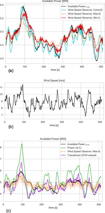
116                                               T. Göçmen et al.: Model-free estimation of available power using deep learning

                                                                         3.1     Data pre-processing and training strategy

                                                                         The investigated case studies for available power estima-
                                                                         tion are generated and implemented using HAWC2 simula-
                                                                         tions with the DTU 10 MW reference wind turbine. For the
                                                                         training of the LSTM models, the high-frequency (100 Hz)
                                                                         wind speed signals from HAWC2 are down-sampled to 1 Hz,
                                                                         which is equivalent to the supervisory control and data ac-
                                                                         quisition (SCADA) system of a wind turbine (Göçmen and
                                                                         Giebel, 2018). The second input to the model is a moving
                                                                         (or rolling) standard deviation of the 1 Hz wind speed, with a
                                                                         10 min rolling window as an indication of inflow turbulence
                                                                         intensity (TI). In contrast to the regular definition, this ap-
Figure 3. LSTM neuron with cell state ct , as well as input it , out-
                                                                         proximation of TI assures the same number of samples for
put ot and forget ft gates. xt0 and ht indicate the inputs and outputs
                                                                         both of the inputs.
of the neuron, respectively. The curves represent sigmoid gates, σ .
                                                                            The two inputs of wind speed and its moving standard de-
                                                                         viation are first normalized between (0, 1) and then fed to the
corresponding bias vector. The final output of the cell is then          LSTM network to predict the power output during normal
defined using ot and ct via the tanh function by                         operation. As an LSTM neuron expects a three-dimensional
                                                                         input shape on the order of samples, lag and features, the in-
ht = ot tanh (ct ) .                                              (8)    put data are shaped accordingly. For the defined architecture
                                                                         with two input features listed above, the hindsight horizon to
                                                                         base the real-time estimations on is another hyper-parameter
   LSTM algorithms are heavily used in a variety of sequen-              to be tuned. The hindsight horizon, or lag, is the number
tial and temporal predictive modelling, from language pro-               of previous time steps that have been taken into account to
cessing (e.g. Gers and Schmidhuber, 2001) to short-term                  predict the power output in the current time step. Note that
forecasting (e.g. Zhang et al., 2019). However, they require             longer lag would increase the initialization period for the
large amounts of data and computational resources to reach               curtailment implementation and could be a limiting factor
their full potential and achieve a generic solution without              if the architecture is to be further adapted for online learn-
over-fitting. Therefore, although RNNs (and LSTMs in par-                ing/training. Accordingly, for the LSTM networks the lags
ticular) have additional capabilities of modelling longer-term           of 4, 9, 29, 59 and 89 s are investigated. Note that since the
temporal properties, they remain highly challenging to train,            model is trained to map the atmospheric inputs to the actual
especially with limited training data. In recent years, the              production data under normal operation, the power predic-
transfer learning (or knowledge transfer) approach that ad-              tions are ensured to follow the normal operation trend that is
dresses such problems (Pan and Yang, 2010) has been in-                  required for the available power estimation and not affected
creasingly popular. The basic idea of the transfer learning is           by the curtailment strategy.
that a well-trained model and its hyper-parameters that in-                 For the preliminary evaluation of the training and hyper-
volve rich knowledge of the target task can be used to guide             parameter tuning of the model, a split validation dataset is
the training of other models.                                            generated. The final test of the model is based on an indepen-
   Throughout the rest of this section, we will firstly present          dent time series with a similar mean wind speed and turbu-
the details of the architecture and the hyper-parameter tuning           lence intensity but covers a shorter time period. Since the tar-
of an LSTM model fully trained on 3 h of HAWC2 simula-                   get application of the model is to estimate real-time available
tions and compare the initial performance of LSTM neurons                power for more certain delta control (or reserve provision),
with simpler perceptrons in FFNN. We will then challenge                 the main criteria of evaluation is the 1 Hz error distribution
our LSTM network to perform on another case with a dif-                  for shorter test cases (10 min), where grid code compliance is
ferent inflow condition than the original training domain. In            tested for longer available periods (1 h) based on 1 min error
pursuit of better performance on a different flow case, we will          distributions.
present the results from blind training as well as the transfer
learning. We will then discuss their behaviour in terms of
both the resulting error distributions and fitted parameters in
                                                                         3.1.1    Training of the first LSTM model: low wind speed,
between the layers. Finally, we will extend the application of
                                                                                  high turbulence intensity
the transfer learning to other flow cases, to demonstrate the
flexibility and automation of the approach.                              The case study to train the first LSTM model consists of a
                                                                         3 h period, where hub-height wind speed and corresponding
                                                                         moving TI are used to estimate the power output of DTU

Wind Energ. Sci., 6, 111–129, 2021                                                           https://doi.org/10.5194/wes-6-111-2021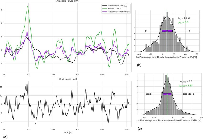
T. Göçmen et al.: Model-free estimation of available power using deep learning 117
Table 1. Representative grid search for best architecture of the first
network using feed-forward neural networks (FFNNs) and LSTM
with lag = 29 s and tanh activation function in between the hidden
layers. Both FFNN and LSTM trained using the Adam optimization
algorithm and mean absolute error loss function. The listed percent-
age error estimation with mean µerr and standard deviation σerr is
y −yobservation
based on the validation dataset where prediction
yobservation × 100.
No. of neurons
Architecture µerr [%] σerr [%]
Layer 1 Layer 2 Layer 3
FFNN 3.1 13.4
50 50 –
LSTM 0.8 10.1
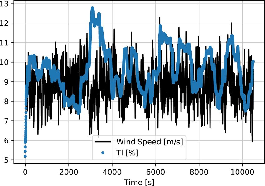
Figure 4. First LSTM model training input time series generated FFNN 1.1 13.3
100 100 –
by HAWC2, down-sampled to 1 Hz. Mean wind speed = 7 m s−1 ; LSTM 0.7 10.1
mean TI = 10 %. FFNN 3.0 13.6
50 50 50
LSTM 0.5 10.0
FFNN 2.0 13.5
50 100 50
LSTM 0.3 10.1
FFNN 1.8 13.7
100 100 50
LSTM 0.3 9.9
ceptrons and LSTM neurons with lag = 29 s. It shows over-
all higher performance for LSTM configurations, indicating
added value of using neurons with memory capabilities. In
fact, LSTM is shown to also outperform more modern ar-
chitectures such as extreme learning machine (ELM) (Saini
et al., 2020) and Gaussian mixture models (GMMs) (Zhang
et al., 2019) for short-term forecasting. Given the best over-
all performance, the final network has three hidden layers
with 100, 100 and 50 LSTM neurons, as detailed in Table 2.
Figure 5. Training history of the first LSTM network with mean The hyperbolic tangent function, tanh, is used as the acti-
wind speed = 7 m s−1 , mean TI = 10 % and time lag = 29 s. The vation function in between the layers. With the listed input
network architecture is presented in Table 2, where batch size = 60 structure, the final architecture corresponds to approximately
with Adam optimization algorithm and mean absolute error (MAE) 7 times more data than the trainable parameters, slightly less
loss function implemented. The training is stopped at epoch = 100, than the general rule of thumb to avoid overfitting; hence
after which the network training starts to show symptoms of overfit. even higher numbers of neurons are avoided. Nevertheless,
the training history in Fig. 5 and the model performance on
the validation dataset do not indicate a clear overfit, increas-
10 MW turbine under nominal operation. The input time se- ing confidence in the training. For the mean absolute error as
ries are presented in Fig. 4. the loss function, the training history on the very first epoch
In order to have an adequate quantity of training sam- for validation data shows “too good” performance of the ini-
ples while assuring a representative test dataset for hyper- tial fit. However, since it clearly does not indicate an overall
parameter tuning, the 3 h period of training and validation higher accuracy, the network is trained further to its fuller
signals is split as 80 % and 20 %, respectively. Since the tar- potential, where the validation loss is expectedly lower and
get available power output is 1 Hz, the final model needs to convergence is achieved around 100 epochs.
be able to handle high-frequency dynamics in the inflow and The first LSTM network is tested on a separate 10 min
successfully map it to the produced power in normal opera- dataset and compared with the true available power (actual
tion, by taking the inertia into account. Given the complex- production of the DTU 10 MW turbine under normal op-
ity the model is required to manage, the minimum number eration) as well as the predecessor method of pre-defined
of neurons per layer is kept at 50 where two to three hid- CP look-up tables of the same turbine. The 1 Hz time series
den layers are evaluated as candidate architectures. Table 1 and the corresponding 1 s percentage error distribution of the
compares the performance of different network configura- direct CP look-up table approach and the LSTM model re-
tions on validation data, for both more traditional FFNN per- sults with lag = 29 s are presented in Fig. 6. The sensitivity of
https://doi.org/10.5194/wes-6-111-2021 Wind Energ. Sci., 6, 111–129, 2021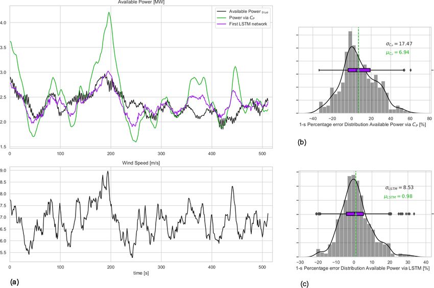
118                                            T. Göçmen et al.: Model-free estimation of available power using deep learning

Figure 6. (a) The 1 Hz time series of available power and wind speed for the first test case: second-wise comparison of the available power
of the 10 MW turbine for mean wind speed = 7 m s−1 and mean TI = 10 % flow case represented in Fig. 4. (b) Available power estimation
error via direct CP curve interpolation of wind speed; (c) error distribution of the first LSTM model with lag = 29 s. µ and σ are the mean
and the standard deviation of the 1 Hz percentage error distributions.

Table 2. Architecture of the first LSTM network with lag = 29 s.        Table 3. Sensitivity of the first LSTM model to the hindsight hori-
Hidden layers: lstm_1, lstm_2, lstm_3. Output layer:                    zon, evaluated based on test dataset.
Dense_1. tanh is used as the activation function in between the
hidden layers.                                                                           Lag      µLSTM [%]     σLSTM [%]
                                                                                         4s            2.52         14.10
 Layer        No. of neurons                   No. of parameters
                                                                                         9s            1.87         14.67
 lstm_1       100                                         41 200                         29 s          0.98          8.53
 lstm_2       100                                         80 400                         59 s         −1.56         12.02
 lstm_3       50                                          30 200                         89 s          0.48         13.21
 Dense_1      1                                               51
              Total parameters: 151 851
              Trainable parameters: 151 851
              Non-trainable parameters: 0                               the mean, µLSTM , and the standard deviation, σLSTM , to the
                                                                        hindsight horizon up to 89 s is listed in Table 3. Due to high-
                                                                        est overall performance, the results from the LSTM model
                                                                        with lag = 29 s will be discussed from now on.
                                                                           Figure 6 shows that the LSTM model significantly im-
                                                                        proves the agreement between the actual and the predicted
                                                                        available power production compared to the direct CP curve
                                                                        interpolation. Since both the trained LSTM model and the
                                                                        CP curve interpolation approach use the same input (hub-

Wind Energ. Sci., 6, 111–129, 2021                                                              https://doi.org/10.5194/wes-6-111-2021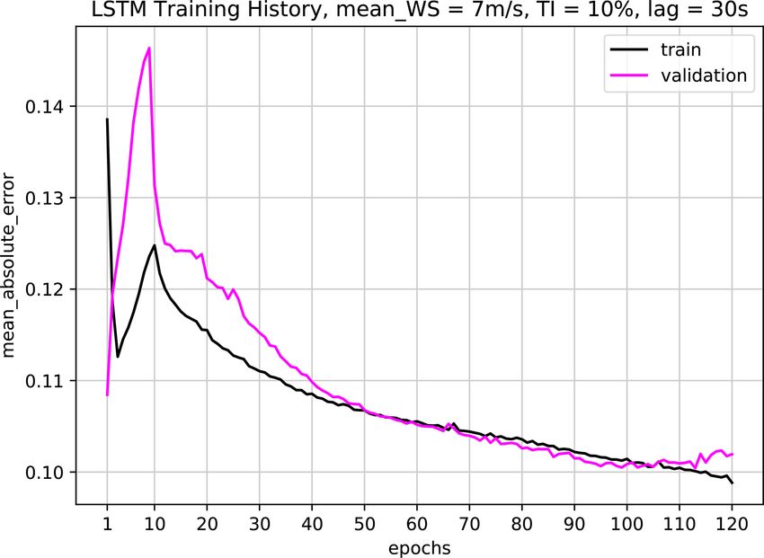
T. Göçmen et al.: Model-free estimation of available power using deep learning                                                 119

height wind speed), it can be said that the described deep-
learning architecture is much more capable of reproducing
the dynamic power curve of the turbine than the steady-state
CP surface, even with limited information. For the investi-
gated 10 min period, the bias in the second-wise LSTM avail-
able power predictions is less than 1 %, as opposed to nearly
7 % observed with the direct CP interpolation approach,
                                              )−y(ti )
where the percentage error is defined as ŷ(tiy(t i)
                                                       × 100 with
y(ti ) being the power produced by DTU 10 MW under nor-
mal operation, i.e. available power, and ŷ(ti ) is the LSTM
model prediction at every time step ti . The standard devia-
tion of the second-wise error distribution, which is regarded
as an indication of uncertainty in the model results for this
                                                                    Figure 7. Second LSTM model training input time series generated
study, is also reduced significantly to 8.5 %. Note that it is      by HAWC2, down-sampled to 1 Hz. Mean wind speed = 9 m s−1 ;
expected to further decrease when the available power pre-          mean TI = 10 %.
diction is to be delivered at larger timescales (e.g. highest
frequency being the 1 min scale as requested by the German
                                                                    Table 4. Sensitivity of the second LSTM model to the hindsight
TSOs; 50Hertz, Amprion, Tennet, TransnetBW, 2016). This             horizon.
will be discussed further for larger evaluation periods later in
the study.                                                                            Lag    µLSTM [%]   σLSTM [%]
                                                                                      4s       3.76            13.45
3.1.2   Training of the second LSTM model: high wind                                  9s       3.85            12.83
        speed, high turbulence intensity                                              29 s     3.83              8.3
                                                                                      59 s     3.15            11.09
One of the most crucial challenges of purely data-driven                              89 s     3.51            12.14
models is the fact that they are not valid for the input vari-
ables outside the training domain, also referred to as the gen-
eralization problem. As seen in Fig. 4 the first LSTM model
is trained for a mean wind speed of 7 m s−1 , where the turbu-      necessarily the best configuration for slightly higher wind
lent fluctuations occasionally reach above 8 m s−1 . However,       speed cases. That trend makes it challenging to develop a
for higher wind speeds, e.g. around 9 m s−1 , the first LSTM        generic network architecture that would successfully repro-
model is expected to perform poorly as it has not been taught       duce the high-frequency available power for all the possible
to map the relationship between wind speed, TI and power            input realizations. It indicates the need to specifically tune
for that inflow.                                                    the hyper-parameters for each separate flow case. It is a
   In order to reduce the effort in hyper-parameter tuning and      cumbersome process with high computational cost. Here in
test the universality of the network architecture for a sim-        this study, the focus is to make the best out of the available
ilar problem, the same configuration as in Table 2 is imple-        dataset, as indicated earlier, as the generation (or collection)
mented with the inflow time series presented in Fig. 7. The fi-     of a comprehensive database is a very demanding task
nal model is referred to as the second LSTM model through-          for high-frequency problems. Additionally, the observed
out this study.                                                     reduction in performance of the same hyper-parameter space
   The performance of the second model is evaluated based           for a different flow case indicates the risk of the approach
on an independent 10 min series with similar mean wind              where a singular “generic” model is fit to estimate the
speed and TI and compared with the direct CP interpolation          high-frequency available power for a variety of inflow cases.
approach. Similar to the first LSTM model, the test results         In other words, a single model to cover the entire domain
are presented for lag = 29 s in Fig. 8.                             might introduce compromises in the model performance at
   Despite the significant performance improvement                  certain inflow cases, where the dynamic accuracy is of the
achieved for the 7 m s−1 case with the first LSTM observed          utmost importance, as framed by the grid codes.
in Fig. 6, the second LSTM network developed using the
same procedure for 9 m s−1 inflow has a considerable bias           3.1.3      Transfer learning from the first model: high wind
of more than 3 % as seen in the 1 Hz percentage error                          speed, high turbulence intensity
distribution in Fig. 8. The mean of the test error seems
to be hardly affected by the changing hindsight horizon             Having trained a well-performing model for the first inflow
listed in Table 4, where the standard deviation is the least at     case with 7 m s−1 mean wind speed and 10 % mean TI, the
lag = 29 s. This clearly implies that the architecture and the      following question arises: can some of the characteristics of
hyper-parameters optimized for the lower wind speed are not         the first model be conveyed to a different flow case to achieve

https://doi.org/10.5194/wes-6-111-2021                                                        Wind Energ. Sci., 6, 111–129, 2021
120 T. Göçmen et al.: Model-free estimation of available power using deep learning Figure 8. (a) The 1 Hz time series of available power and wind speed for the second test case: second-wise comparison of the available power of the 10 MW turbine for mean wind speed = 9 m s−1 and mean TI = 10 % flow case represented in Fig. 7. (b) Available power estimation error via direct CP curve interpolation of wind speed; (c) error distribution of the second LSTM model with lag = 29 s. µ and σ are the mean and the standard deviation of the 1 Hz percentage error distributions. similarly good results? Transfer learning can provide a valu- 0.05 for both. On the other hand, the third and shallower able platform for such model extensions, as it is used to im- layer lstm_3 seems to optimize for significantly different prove a learner from one domain by transferring information weights for different inflow velocities. Therefore, it is con- from a related domain (Weiss et al., 2016). This enables a cluded that the first two LSTM layers are transferable from systematic model update when new data are available from the first LSTM network, where the last LSTM layer as well outside the training domain. Accordingly, part of the first as the output layer need to be re-tuned for changing inflow model with 7 m s−1 mean wind speed would be transferred case(s). The resulting architecture is presented in Table 5 to update some of the parameters for higher wind speed. The where the number of trainable parameters is significantly re- procedure could be repeated for all the changing wind speed duced. Accordingly, the transferred architecture is a much and TI cases, in both HAWC2 platform and field applica- lighter network that ensures fast training, while enclosing a tions. profound amount of information from previous learning(s). To assess the transferability of the parameters, the trends Fewer parameters also enables a robust training with shorter of the weights trained for the first (Network_1) and the Sec- time series. Hence, for the training of the transfer learning ond (Network_2) LSTM networks are compared in Fig. 9. LSTM architecture, 60 % of the dataset (second inflow case, The actual probability seen in the most recent histograms (the presented in Fig. 7) is fed to the network, where 40 % is left lightest shade in the series of distributions) are different for for validation to ensure a more definitive assessment of the all three LSTM layers, with larger tails on Network_1 distri- training. butions. However, the range of values for the output weights Apart from an update of the weights in the last LSTM and of the first layer lstm_1 and the second layer lstm_2 are the output layers (lstm_4 and Dense_2 in Table 5, respec- very similar, with an interquartile range of −0.05 < IQR < tively), none of the other hyper-parameters were changed in Wind Energ. Sci., 6, 111–129, 2021 https://doi.org/10.5194/wes-6-111-2021
T. Göçmen et al.: Model-free estimation of available power using deep learning                                                       121

Figure 9. Distribution of the output tensors of each hidden LSTM layer for the first Network_1 and the second Network_2 LSTM networks,
visualized via TensorBoard. Each slice displays a single histogram updated at each iteration. The “oldest” iterations are further back and
darker, while the “newer” ones are lighter and closer to the front. The y axis indicates the relative time of each update.

Table 5. Architecture of the transferred LSTM network for               the training process of the transferred LSTM network. This
lag = 29 s. Hidden layers: LSTM_1, LSTM_2, LSTM_4. Output               provides a certain repeatability to the training process, where
layer: Dense_2. Frozen layers: LSTM_1, LSTM_2 (same layers              the last two layers can be updated when a new flow case is
as in the first LSTM model in Table 2). Trainable layers: LSTM_4,       encountered by the turbine. It is particularly an important fea-
Dense_2. tanh is used as the activation function in both of the acti-   ture for the control implementation as it enables fast online
vation layers. Training is performed with batch size = 60, the Adam
                                                                        learning and continuous improvement of the model.
optimization algorithm and a mean absolute error loss function over
epoch = 70.
                                                                           To put the performance of the transferred LSTM model to
                                                                        the test, the same test case as in the second LSTM model
 Layer        No. of neurons                      No. of parameters     in Fig. 8 is considered. This time, the estimations from the
                                                                        operation-dependent wind speed observer (WSO) approach
 lstm_1       100                                           41 200
                                                                        (described in Sect. 2) are also compared with the transferred
 lstm_2       100                                           80 400
 lstm_4       50                                            30 200      LSTM model. The time series in Fig. 10a illustrates the sensi-
 Dense_2      1                                                 51      tivity of the WSO estimations to the operation strategy under
              Total parameters: 151 851
                                                                        40 % down-regulation with constant rotational speed, Const-
              Trainable parameters: 30 251                              , and maximum rotational speed, Max-, and following
              Non-trainable parameters: 121 600                         the minimum thrust coefficient, Min-Ct . In Fig. 11a–c, the
                                                                        error distributions of the WSO estimations under those three
                                                                        operational strategies are presented. While the overall perfor-

https://doi.org/10.5194/wes-6-111-2021                                                          Wind Energ. Sci., 6, 111–129, 2021
122 T. Göçmen et al.: Model-free estimation of available power using deep learning
mance of all WSO estimations is highly compelling, the re-
sults also indicate up to 4 % variation in the mean bias of the
WSO model. With the minimum mean error of 0.26 %, WSO
estimations with maximum rotational speed, Max-, are also
compared with the transferred LSTM model in Fig. 10c. For
the investigated setup with the DTU 10 MW reference tur-
bine model fully recognized, the WSO results generally sug-
gest a better agreement with the true available power, quan-
tified in Fig. 11d. However, Figs. 10c and 12 point out that
for a potential mismatch of 5 % in the pre-defined and op-
erational CP surfaces due to several uncertainties listed ear-
lier, model-based WSO results show bias of up to more than
6 % where the model-free LSTM performance remains un-
affected. Note that in these WSO runs, we assume “perfect
knowledge” for normal operation, i.e. for maximum CP , and
5 % uncertainty for the rest of the CP domain. This simu-
lates the field operation where the nominal power curve is
corrected for the site conditions (hence perfect knowledge)
but the information of the rest of the operational CP remains
limited.
It is also seen that the transferred LSTM model outper-
forms the second LSTM model where more than 3 % model
bias is eliminated compared to Fig. 8d. This improvement is
very promising for the implementation of the transfer learn-
ing for modelling high-frequency time series with LSTM net-
works. Furthermore, the results also show the potential of
such a deep-learning approach for avoiding the operational
dependencies of dynamic delta control with relatively low
uncertainties. The adaptation capabilities of transfer learning
are to be tested with additional flow cases in the next sec-
tions.
3.1.4 Further transfer learning to higher wind speed
flows
With the comparable results of the model-free transfer learn-
ing LSTM networks to the model-dependent WSO approach,
even with potentially lower uncertainties in the simulation
environment compared to the field implementation, here we
test the approach for even higher wind speed flows. The first
LSTM predictions were built and tested on 7 m s−1 mean
wind speed, where its information from the first two layers
is then transferred to estimate the available power for the Figure 10. The 1 Hz time series comparison of available power
9 m s−1 mean wind speed case. Here we further update the of DTU 10 MW turbine, estimated by (a) the wind speed observer
LSTM network to extend the training (and validity) domain for the 40 % down-regulation case under three different curtailment
strategies; see Sect. 2. (b) Second-wise wind speed time series of
to the 11 m s−1 mean wind speed range, using the generated
the considered test case with mean wind speed = 9 m s−1 and mean
time series in Fig. 13. Note that for all three steps of the learn-
TI = 10 %. (c) The comparison of the available power estimated via
ing, the mean TI remains 10 % to isolate the effect of wind wind speed observer following the maximum rotational speed con-
speed on the network performance. trol strategy and LSTM network with transfer learning from the
The resulting network with further transfer learning for lower wind speed to higher wind speed cases and direct CP ap-
11 m s−1 mean wind speed (in Fig. 14a) performs similar to proach. The shaded area corresponds to the effects of ±5 % over-
in the 9 m s−1 (in Fig. 11d) and 7 m s−1 (in Fig. 6d) mean and underestimation of CP during curtailment for WSO results. The
wind speed cases with less than 1 % second-wise percentage LSTM network has no dependency on level of curtailment or esti-
error on average. Distinctly from the previous inflow cases, mation of operational CP .
the tail towards the positive percentage error is longer in the
Wind Energ. Sci., 6, 111–129, 2021 https://doi.org/10.5194/wes-6-111-2021T. Göçmen et al.: Model-free estimation of available power using deep learning 123 Figure 11. The 1 Hz percentage error distribution of the available power estimation of the 10 MW turbine for mean wind speed = 9 m s−1 and mean TI = 10 %, the flow case represented in Fig. 7. The presented performances belong to the wind speed observer approach, presented in Sect. 2, under different operational strategies. (a) Constant rotational speed, Const.-; (b) maximum rotational speed, Max-; (c) minimum thrust coefficient, Min-Ct , as 40 % curtailment strategy; (d) LSTM model with transfer learning from lower wind speed to the higher wind speed case (no dependency on the curtailment strategy). Figure 12. (a) Sensitivity of wind speed observer to correct assessment of CP under curtailment. The simulations assume “perfect knowl- edge” of CP for the normal operation and 5 % uniform uncertainty for the rest of the operational range. (a) The 1 Hz percentage error of WSO with Max-: 5 % under-estimation of CP during curtailment. (b) The 1 Hz percentage error of WSO with Max-: 5 % over-estimation of CP during curtailment. final 1 Hz error distribution in Fig. 14a. This is mainly due 1 min scale in Fig. 14b. The results show that the model-free to the fact that the DTU 10 MW reference turbine (with rated transfer learning approach easily complies with the strictest wind speed 11.4 m s−1 ) occasionally enters the rated region TSO requirements in provision of the available power signal; according to the turbulent fluctuations around 11 m s−1 mean i.e. the standard deviation of the 1 min percentage error of the wind speed. Nevertheless, the variability of the model pre- available power is required to be less than ±3.3 % as stated diction error is significantly reduced when averaged for a in 50Hertz, Amprion, Tennet, TransnetBW (2016). https://doi.org/10.5194/wes-6-111-2021 Wind Energ. Sci., 6, 111–129, 2021
124                                          T. Göçmen et al.: Model-free estimation of available power using deep learning

                                                                  shown to comply with the strictest grid code requirements
                                                                  under different turbulence realizations.

                                                                  4   Conclusions

                                                                  The dynamic estimation of available power of a wind turbine
                                                                  is essential for both power system stability and marketabil-
                                                                  ity of the reserve power. The current estimations are highly
                                                                  sensitive to the down-regulation strategy and prone to tur-
                                                                  bine model uncertainties and inadequacies. Here we propose
                                                                  a purely data-driven, model-free methodology based on long
                                                                  short-term memory (LSTM) neural networks. This state-of-
Figure 13. LSTM network training with further transfer learning
                                                                  the-art deep-learning architecture is implemented to map the
input time series generated by HAWC2, down-sampled to 1 Hz.
                                                                  available power of the DTU 10MW reference turbine under
Mean wind speed = 11 m s−1 ; mean TI = 10 %.
                                                                  turbulent inflow generated in HAWC2. The trained networks
                                                                  are adapted to the changes in incoming mean wind speed via
3.1.5   Network performance on higher turbulence                  transfer learning, where only the parameters in the last layer
        intensity                                                 are updated when the new inflow information is available.
                                                                     The first LSTM network has three hidden layers with 100,
As stated earlier, for all three inflow cases where the first     100 and 50 neurons which is trained using 1 Hz power output
LSTM network is generated and extended via transfer learn-        under normal operation with 7 m s−1 mean wind speed and
ing, the mean turbulence intensity remained TI = 10 %. Here       10 % turbulence intensity (TI). A performed test on a sep-
in this section, the models are tested under higher turbu-        arate 10 min flow case with the same mean wind speed and
lence intensity (TI = 20 %) with the same corresponding           TI shows less than 1 % bias and less than 9 % standard devia-
mean wind speed. Note that the generated network structures,      tion. The same architecture is used to train the second LSTM
i.e. the first LSTM model (7 m s−1 mean inflow speed), trans-     network with an increase in mean wind speed to 9 m s−1 and
fer learning LSTM model (9 m s−1 mean inflow speed) and           the same TI level of 10 %. Although the width of the distribu-
further transfer learning LSTM model (11 m s−1 mean inflow        tion is similar, the bias has increased to almost 4 %, indicat-
speed), are not updated for higher-TI cases. In other words,      ing the need to re-tune the hyperparameters of the architec-
here we aim to test the capability of the trained networks un-    ture. In fact, the comparison of the fitted parameters between
der higher TI with the same mean wind speed for the inflow,       the first LSTM and the second LSTM networks for each layer
without further model update.                                     shows analogous distributions of the weights. This further
   Figures 15–17 focus on highly turbulent inflow cases           motivates the transferability of the learnings of the first two
(TI = 20 %) and show the corresponding performance of the         LSTM layers, where only the parameters of the last layer
three neural networks trained and updated for increasing          need to be updated for the changing incoming mean wind
wind speeds via transfer learning. It is seen that the 1 min      speed. With a significant reduction in the number of param-
average prediction errors of the models are consistently low      eters to fit, the transferred LSTM network has the capability
for highly turbulent flows as well; hence further training (or    of faster and more robust training, even with limited data.
model update) is not required. The maximum standard de-           The performance of the transferred LSTM network is also
viation of 1 min averaged percentage error is still less than     evaluated using a separate 10 min time series with 9 m s−1
3.3 % with the largest bias of 1.3 %, which is slightly worse     mean wind speed and 10 % TI. The results are very com-
than the test results in the original domain of the networks.     parable with the outcome of the first LSTM model, which
For the mean wind speeds of 7 and 9 m s−1 , the effect of         demonstrates the adaptability of the network to changing in-
higher turbulence levels is clearer as increasing fluctuations    flow conditions with the update of the last LSTM layer. The
in wind speed are directly correlated to higher variance in       transferred LSTM also outperforms the second LSTM net-
power output. However for the 11 m s−1 case, the fluctua-         work with a significant decrease in bias (around 0.5 %), elim-
tions are partially dampened due to the turbine entering into     inating the need to re-tune the hyperparameters or developing
the rated region. Overall, it can be said that the sensitivity    a new network structure from scratch.
of the networks to changing wind speed is much higher than           The transferred LSTM network is also compared with
the turbulence, and the updates are to be implemented solely      the model- and operation-dependent wind speed ob-
based on the altering inflow velocity, which is likely to re-     server (WSO) approach. For the investigated setup where the
flect a different operational region. The available power pre-    DTU 10 MW reference turbine model is fully transparent or
diction of the described LSTM architecture and the updating       known, the WSO results generally suggest a better agreement
scheme with 2 m s−1 wind speed increase (7–9–11 m s−1 ) is        with narrower 1 Hz percentage error distributions. However,

Wind Energ. Sci., 6, 111–129, 2021                                                   https://doi.org/10.5194/wes-6-111-2021
You can also read