A new dense 18-year time series of surface water fraction estimates from MODIS for the Mediterranean region - HESS
←
→
Page content transcription
If your browser does not render page correctly, please read the page content below
Hydrol. Earth Syst. Sci., 23, 3037–3056, 2019
https://doi.org/10.5194/hess-23-3037-2019
© Author(s) 2019. This work is distributed under
the Creative Commons Attribution 4.0 License.

A new dense 18-year time series of surface water fraction estimates
from MODIS for the Mediterranean region
Linlin Li1 , Andrew Skidmore1,2 , Anton Vrieling1 , and Tiejun Wang1
1 Faculty   of Geo-information Science and Earth Observation, University of Twente, Enschede, the Netherlands
2 Department    of Environmental Sciences, Macquarie University, NSW, Australia

Correspondence: Linlin Li (l.li-1@utwente.nl, jane09gis@gmail.com)

Received: 2 January 2019 – Discussion started: 28 January 2019
Revised: 24 June 2019 – Accepted: 25 June 2019 – Published: 17 July 2019

Abstract. Detailed knowledge on surface water distribution        ment of the seasonal, inter-annual, and long-term variability
and its changes is of high importance for water management        of water resources, inclusive of small water bodies.
and biodiversity conservation. Landsat-based assessments of
surface water, such as the Global Surface Water (GSW)
dataset developed by the European Commission Joint Re-
search Centre (JRC), may not capture important changes in         1   Introduction
surface water during months with considerable cloud cover.
This results in large temporal gaps in the Landsat record that    Terrestrial surface water bodies such as lakes, reservoirs, and
prevent the accurate assessment of surface water dynamics.        rivers cover approximately 3 % of the global land mass. They
Here we show that the frequent global acquisitions by the         play a crucial role in the global hydrological cycle, biodiver-
Moderate Resolution Imaging Spectrometer (MODIS) sen-             sity conservation, and climate process (Chahine, 1992; Tran-
sors can compensate for this shortcoming, and in addition         vik et al., 2009). Detailed knowledge on surface water distri-
allow for the examination of surface water changes at fine        bution, and its seasonal, inter-annual, and long-term variabil-
temporal resolution. To account for water bodies smaller than     ity can serve as an important source for water management
a MODIS cell, we developed a global rule-based regression         (Cole et al., 2007), ecosystem assessment, and biodiversity
model for estimating the surface water fraction from a 500 m      conservation (Turak et al., 2017). Remote-sensing data have
nadir reflectance product from MODIS (MCD43A4). The               increasingly been used to monitor surface water changes, and
model was trained and evaluated with the GSW monthly wa-          powerful methods and tools have been developed for analyz-
ter history dataset. A high estimation accuracy (R 2 = 0.91,      ing Earth observation data. However, existing approaches for
RMSE = 11.41 %, and MAE = 6.39 %) was achieved. We                monitoring the surface water extent are limited either in geo-
then applied the algorithm to 18 years of MODIS data (2000–       graphic scope, temporal extent of the record, or with respect
2017) to generate a time series of surface water fraction maps    to the temporal frequency of observations.
at an 8 d interval for the Mediterranean. From these maps            At the global scale, several static datasets exist that provide
we derived metrics including the mean annual maximum,             information on the spatial extent of water bodies and wet-
the standard deviation, and the seasonality of surface water.     lands. For example, the Global Lakes and Wetlands Database
The dynamic surface water extent estimates from MODIS             (GLWD: Lehner and Doll, 2004) was based on historical
were compared with the results from GSW and water level           maps and has a spatial resolution of 30 arcsec (approx. 1 km).
data measured in situ or by satellite altimetry, yielding simi-   Carroll et al. (2009) combined the Shuttle Radar Topogra-
lar temporal patterns. Our dataset complements surface water      phy Missions (SRTM) Water Body Data (SWBD) with 250 m
products at a fine spatial resolution by adding more tempo-       Moderate Resolution Imaging Spectrometer (MODIS) re-
ral detail, which permits the effective monitoring and assess-    flectance data to produce a global static map of surface water
                                                                  for circa 2000–2002. Global Landsat-based static surface wa-
                                                                  ter datasets include the 3 arcsec (∼ 90 m) Water Body Map

Published by Copernicus Publications on behalf of the European Geosciences Union.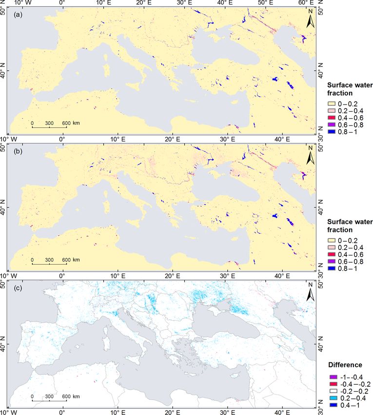
3038                                         L. Li et al.: A new dense 18-year time series of surface water fraction estimates

(G3WBM: Yamazaki et al., 2015) and the Global Land Cover            hanced our understanding of rapid water changes caused by
Facility (GLCF) inland surface water dataset at a 30 m reso-        extreme climate change and human activities. However, like
lution for 2000 (Feng et al., 2015).                                other surface water mapping efforts based on binary classifi-
   Even though static water maps are adequate for some ap-          cation methods (e.g., Khandelwal et al., 2017; Mohammadi
plications there is an increasing demand for information on         et al., 2017), this product omits lakes and narrow rivers that
the spatiotemporal variability of inland water bodies and           only cover a portion of a MODIS resolution cell.
their long-term evolution (Belward, 2016). Dynamic map-                To overcome this limitation and incorporate small water
ping and monitoring of the surface water extent have been           bodies, several researchers have attempted to predict sub-
explored using optical sensors featuring fine (10–30 m) to          pixel surface water estimates of MODIS by providing the
medium (250–500 m) spatial resolutions. At fine spatial reso-       water fraction in each pixel using techniques like linear
lution, several studies have recently presented interesting re-     spectral mixture modeling (e.g., Hope et al., 1999; Li et
sults on long-term variability of surface water with the entire     al., 2013; Olthof et al., 2015) and machine learning (e.g.,
Landsat archive at regional (Halabisky et al., 2016; Heimhu-        Li et al., 2018; Rover et al., 2010; Sun et al., 2012) for
ber et al., 2016), continental (Mueller et al., 2016), and global   small areas. However, the utility and efficiency of these meth-
scales (Donchyts et al., 2016; Pekel et al., 2016). The Eu-         ods have rarely been explored for the estimation of the sur-
ropean Commission Joint Research Centre’s (JRC) Global              face water fraction for larger areas. In our previous work (Li
Surface Water (GSW) dataset (Pekel et al., 2016) quantifies         et al., 2018), we explored the use of rule-based regression
changes in global surface water over the past 32 years with         models over two small areas on the Iberian Peninsula and
a monthly time interval. This product allows for the analy-         concluded that a single global regression model can provide
sis of surface water dynamics over long time periods at fine        accurate surface water estimates across areas with different
spatial resolution, but only provides information on monthly        environmental conditions as long as it is fed with training
changes in surface water. Moreover, the Landsat archive also        data that comprise these various conditions. Consequently,
contains data gaps and temporal discontinuities depending           we concluded that this approach has the potential to be ap-
on the geographical location (Pekel et al., 2016). This is due      plied over much larger areas. Therefore, the aim of this paper
to both the limited number of acquisitions during specific          is to explore the utility and efficiency of a rule-based regres-
time intervals, and the location- and time-dependent persis-        sion model for the estimation of the surface water fraction for
tency of cloud cover. These data gaps affect the accuracy           the Mediterranean region, and to develop a new surface wa-
of the seasonality information (Yamazaki and Trigg, 2016).          ter fraction dataset for the Mediterranean region using fine
To better represent water bodies with short hydroperiods and        temporal resolution MODIS data as input for the effective
short-duration flooding, it is critical to account for such gaps    assessment of seasonal, intra-annual, and long-term surface
when monitoring surface water. In recent years, the revisit         water dynamics inclusive of small water bodies. Our specific
time of fine-resolution sensors has increased (e.g., Sentinel-2     objectives are as follows:
has offered a 5 d repeat since March 2017: Du et al., 2016).
However, these data cannot yet be used to create long-term              1. to develop an approach for the estimation of the sur-
(> 10 year) consistent time series at short time intervals.                face water fraction for the Mediterranean region at a fine
   Moderate resolution imagery derived from satellite sen-                 temporal resolution from MODIS data;
sors such as MODIS provides daily observations over long
                                                                        2. to generate an 8 d interval time series of surface water
time-spans and as such has the potential to construct long-
                                                                           fraction maps for the Mediterranean from 2000 to 2017,
term and dense time series of surface water over large re-
                                                                           and to use that to derive a series of ecologically relevant
gions. Many studies have explored the use of MODIS in
                                                                           metrics;
mapping water body dynamics at regional to continental
scales (Kaptue et al., 2013; Pekel et al., 2014; Sharma et              3. to compare our dataset with an existing dataset (i.e.,
al., 2015) using binary classification methods. At the global              JRC’s GSW) and water level data to assess how they
scale, Khandelwal et al. (2017) used MODIS multispectral                   compare in space and time.
data to map the global extent and temporal variations of
94 large reservoirs at a 500 m resolution and at an 8 d in-
terval from 2000 to 2015. The recent Global Climate Ob-             2    Study area
serving System (GCOS) report states that essential climate
variables (ECVs) need to be established for water extent and        We loosely defined the Mediterranean in this study as the
lake ice cover products, ideally with daily temporal resolu-        region that is contained within 10 MODIS grid tiles, which
tion (Belward, 2016). To address this requirement, the first        together cover all coastal areas of the Mediterranean and the
daily global dataset of inland water bodies at a 250 m spa-         Black Sea, including a significant portion of their inland ar-
tial resolution from 2013 to 2015 was developed by Klein et         eas (Fig. 1). This boundary is defined based on the combina-
al. (2017). This work advanced surface water mapping using          tion of (1) the definition of the Mediterranean region by the
remote sensing, due to its dense temporal resolution, and en-       Mediterranean Wetland Observatory (MWO) project, i.e., 27

Hydrol. Earth Syst. Sci., 23, 3037–3056, 2019                                       www.hydrol-earth-syst-sci.net/23/3037/2019/
L. Li et al.: A new dense 18-year time series of surface water fraction estimates                                            3039

Mediterranean countries are included by MWO; (2) the in-           3.1   MODIS data
clusion of areas with a large amount of Ramsar wetlands; and
(3) the exclusion of southern parts of north African countries     The main input dataset in this study is the MODIS Terra
(i.e., Morocco, Algeria, Libya, and Egypt) that comprise few       and Aqua nadir BRDF-adjusted reflectance (NBAR) prod-
water bodies according to the maximum water extent over            uct (MCD43A4, V006). This product provides 500 m reso-
32 years from JRC’s GSW product.                                   lution surface reflectance data for each of the MODIS bands
   The study region covers 13 climate zones as defined by          (1–7) corrected to a common nadir view geometry at the lo-
Peel et al. (2007) (Fig. 1). Numerous water bodies of dif-         cal solar noon zenith angle using a bidirectional reflectance
ferent types are found in this region, including large coastal     distribution function (BRDF) model (Schaaf, 2015b). Com-
lagoons, fresh, brackish or salt marshes, riverine forests and     pared with the previous collection (V005) that had an 8 d fre-
reed beds, flood plains and wet meadows, mountainous lakes         quency, the V006 collection was retrieved on a daily basis.
and surrounding wetlands, salted lakes, temporary marshes,         Each daily value is a result of compositing information ob-
and streams (Costa et al., 1996). Our study area accounts for      tained during 16 d of observations, which are weighted as
25 % of the world’s Ramsar sites that contain a great eco-         a function of the quality, the observation coverage, and the
logical, social, and economic value, especially as they pro-       temporal distance from the day of interest. Each daily V006
vide habitat, reproduction, and migration stopover sites for       retrieval is the center (i.e., the ninth day) of the moving 16 d
numerous bird species (Galewski, 2012). A good number of           input window (Schaaf, 2015b). We also used the MCD43A2
the water bodies and wetlands in the region are small, shal-       (V006) Bidirectional Reflectance Distribution Function and
low, and highly variable between seasons and years due to          Albedo (BRDF/Albedo) Quality dataset to filter out pixels
weather effects and human activities (Costa et al., 1996).         with snow and ice in the MCD43A4 product. This dataset
   Many Mediterranean water resources are degraded mainly          has the same temporal and spatial resolution as MCD43A4
due to urbanization, agricultural reclamation, increasing wa-      (i.e., daily 500 m resolution), and contains quality informa-
ter use for irrigation, and hydraulic works such as dams,          tion for the corresponding MCD43A4 NBAR product includ-
dikes, river channeling, and drainage and irrigation networks      ing snow and ice presence (Schaaf, 2015a).
(Batalla et al., 2004). A number of projects and programs             For this study, we downloaded the daily files of MCD43A4
have performed monitoring of surface water and wetlands in         and MCD43A2 for 2000, 2003, 2006, 2009, 2012, and 2015.
the Mediterranean region, such as MWO (http://medwet.org/,         As explained in Sect. 4.1, all the available dates (or months)
last access: 10 July 2019) and the GlobWetland initiative          of the GSW monthly water history dataset in these 6 years
(http://webgis.jena-optronik.de/, last access: 10 July 2019),      over the sample locations were used for building training
which highlighted the importance of protecting Mediter-            and validation data. Instead, when producing the surface wa-
ranean water resources. However, these projects either per-        ter fraction time series, we collected the MCD43A4 and
formed wetland mapping for a few moments in time (e.g.,            MCD43A2 files using an 8 d time step from February 2000 to
GlobWetland only covered 1975, 1990, and 2005), or were            December 2017, as processing daily files for the large study
limited to specific water bodies and wetlands instead of the       area and the 18-year time period would become too time-
whole landscape. Although surface water dynamics in the            and memory-consuming. The 8 d repeat coverage is consid-
Mediterranean can be analyzed at fine spatial resolution with      ered to be a minimum for effectively capturing water bod-
JRC’s GSW, it has large spatial and temporal gaps. Figure 2        ies with short hydroperiods while simultaneously accounting
shows the percentage of pixels with valid observations in          for frequent cloud cover (Guerschmann et al., 2011; Wulder
JRC’s GSW monthly water history dataset for each month             et al., 2016). All images were downloaded from the NASA
between January 2000 and October 2015 calculated over the          Earthdata Search website (https://search.earthdata.nasa.gov/
entire Mediterranean area. The figure illustrates that no valid    search, last access: 10 July 2019).
observation exists for December in the years 2000–2015 in
Mediterranean areas according to the GSW monthly water             3.2   Global Surface Water (GSW) dataset
history map. In addition, less than 10 % of the Mediterranean
area has observations for January.                                 To generate training and validation data for modeling the
                                                                   surface water fraction, we used the GSW dataset (Pekel et
                                                                   al., 2016). This dataset provides the global distribution of
3   Data                                                           the surface water extent at a monthly time interval from
                                                                   March 1984 to October 2015 (380 months) at a 30 m spa-
Table 1 summarizes all datasets used in this study. They in-
                                                                   tial resolution, and also includes a series of thematic maps
clude a number of sources used to derive model input vari-
                                                                   summarizing different facets of the spatial and temporal dy-
ables, training data for building the model, validation data for
                                                                   namics of surface water over 32 years. This dataset is de-
model accuracy assessment, and other existing surface water
                                                                   rived from the entire archive of Landsat 5 Thematic Map-
products against which we compared our products. Details
                                                                   per (TM), the Landsat 7 Enhanced Thematic Mapper-plus
are provided in the following sections.
                                                                   (ETM+), and the Landsat 8 Operational Land Imager (OLI).

www.hydrol-earth-syst-sci.net/23/3037/2019/                                     Hydrol. Earth Syst. Sci., 23, 3037–3056, 2019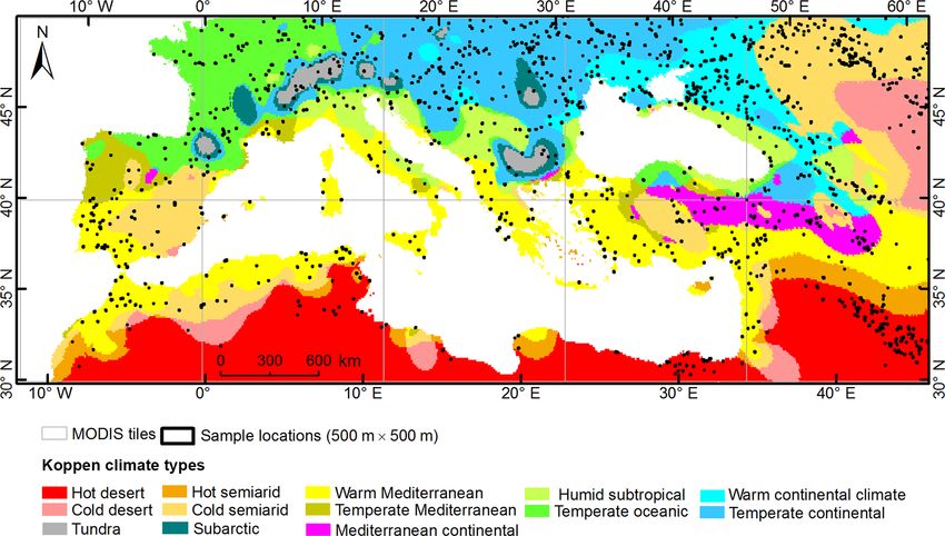
3040                                          L. Li et al.: A new dense 18-year time series of surface water fraction estimates

Figure 1. Study area and sample locations.

                                                                      ping accuracy with a commission accuracy of 99.45 % and
                                                                      an omission accuracy of 97.01 % (Pekel et al., 2016).
                                                                         The GSW monthly water history dataset is available in
                                                                      Google Earth Engine (GEE: Gorelick et al., 2017) as an im-
                                                                      age collection containing 380 images, one for each month be-
                                                                      tween March 1984 and October 2015. Each image provides
                                                                      a binary classification of water presence, or indicates if no
                                                                      valid (cloud-free) Landsat observations were available for a
                                                                      specific pixel and month. For comparison with MODIS data,
                                                                      we used the monthly water history datasets between Febru-
                                                                      ary 2000 and October 2015, which resulted in 189 images.
                                                                         Several GSW thematic maps were derived from the
                                                                      GSW monthly water history dataset (Pekel et al., 2016).
                                                                      In this study, we used two thematic maps, the maxi-
                                                                      mum water extent map and the water transitions map, for
                                                                      the Mediterranean region from the data access website
Figure 2. Percentage of pixels with valid observations in JRC’s       (https://global-surface-water.appspot.com/download, last ac-
Global Surface Water (GSW) monthly water history dataset for each     cess: 10 July 2019). The maximum water extent map indi-
month between January 2000 and October 2015, taken as a spatial       cates whether each 30 m grid cell was ever detected as wa-
average for the entire Mediterranean region as displayed in Fig. 1.   ter over the 32-year period. The transition map contains 10
                                                                      water classes: permanent, new permanent, lost permanent,
                                                                      seasonal, new seasonal, lost seasonal, seasonal to permanent,
Water detection was performed using a dedicated expert sys-           permanent to seasonal, ephemeral permanent, and ephemeral
tem, which was a procedural sequential decision tree that             seasonal. It provides information on both intra- and inter-
used both the multispectral and multitemporal attributes of           annual variability of surface water (Pekel et al., 2016).
the Landsat archive as well as ancillary data layers (Pekel et
al., 2016). Based on a validation with very high resolution
satellite and aerial imagery, the authors reported a high map-

Hydrol. Earth Syst. Sci., 23, 3037–3056, 2019                                      www.hydrol-earth-syst-sci.net/23/3037/2019/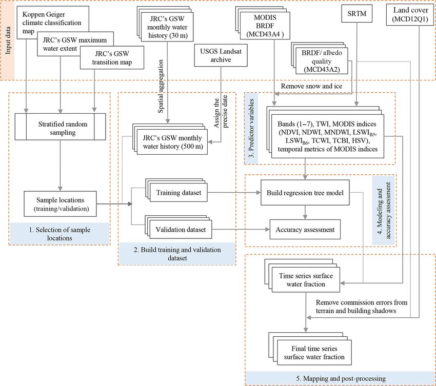
L. Li et al.: A new dense 18-year time series of surface water fraction estimates                                                        3041

Table 1. Input and reference datasets used in the study.

      Data/product name                                    Temporal     Spatial       Purpose in the study
                                                           resolution   resolution
      MCD43A4, V006 (MODIS/Terra and Aqua                  Daily        500 m         Generation of predictor variables and production of
      nadir BRDF-adjusted reflectance)                                                time series of water fraction maps
      MCD43A2, V006 (MODIS/Terra and Aqua                  Daily        500 m         Snow and ice mask
      BRDF/albedo quality)
      GSW monthly water history dataset                    Monthly      30 m          Generation of training and validation datasets, and
                                                                                      thematic products
      GSW maximum water extent map                         Static       30 m          Define sampling strata; exclusion of non-water
                                                                                      samples from training locations
      GSW water transitions map                            Static       30 m          Define sampling strata
      Digital elevation model from Shuttle Radar           Static       90 m          Generation of predictor variables; identification of
      Topography Mission (SRTM) 3 v4.1                                                sloping terrain and terrain shadows
      USGS Landsat archive                                 16 d         30 m          Link the GSW monthly history datasets to a sin-
                                                                                      gle date of cloud-free Landsat acquisition because
                                                                                      the exact date of observation is not included in the
                                                                                      GSW dataset
      MCD12Q1 (MODIS land cover type product)              Static       500 m         Identification of building shadows
      Land water mask derived from MODIS and               Static       250 m         Comparison of products
      SRTM (MOD44W)
      Water level from satellite altimetry                 10 d         –             Validation of results
      Water level from in situ                             Daily        –             Validation of results

3.3   Terrain data                                                          Jason-1, Topex/Poseidon, and ENVISAT satellites. We also
                                                                            obtained daily in situ gauge observations for Fuente de
Terrain data are useful for predicting the locations for wa-                Piedra Natural Reserve in southern Spain, which were also
ter bodies (Drake et al., 2015; Grabs et al., 2009). In this                used in Li et al. (2015).
study, we used the near-global Shuttle Radar Topography
Mission (SRTM) digital elevation model (DEM) distributed                    3.5    Additional data
by the Consortium for Spatial Information of the Consulta-
tive Group of International Agricultural Research (CGIAR-                   We utilized the MODIS land cover type product (i.e.,
CSI). This product has a ∼ 90 m resolution and is a post-                   MCD12Q1: Friedl et al., 2010) to identify and mask ar-
processed derivative to address areas of missing data in the                eas that potentially have commission errors related to build-
original SRTM DEM made by the National Aeronautics and                      ing shadows. To assess the spatial accuracy of MODIS de-
Space Administration (Jarvis et al., 2008). The most recent                 rived maps, we also used the land water mask derived from
version of this product is SRTM3 v4.1 and is freely available               MODIS 250 m and SRTM data (MOD44W: Salomon et
from http://srtm.csi.cgiar.org/ (last access: 10 July 2019).                al., 2004) for comparison.

3.4   Satellite altimetry and in situ water level                           4     Method
We obtained water levels from the U.S. Department of                        4.1    Approach for deriving the surface water fraction
Agriculture Global Reservoir and Lake Monitoring (GRLM)
website        (http://www.pecad.fas.usda.gov/cropexplorer/                 The approach used to derived the surface water fraction
global_reservoir, last access: 10 July 2019). This site                     builds on our previous work (Li et al., 2018) with con-
provides time series of water level variations for some of                  siderable improvements regarding input data, training data,
the world’s largest lakes and reservoirs, mainly greater than               and commission error processing. We explored the use of
100 km2 . The GRLM utilizes near-real time data from the                    MODIS spectral information and a topographic metric for
Jason-3 mission, and archive data from the Jason-2/OSTM,                    estimating the surface water fraction over two study areas in

www.hydrol-earth-syst-sci.net/23/3037/2019/                                                Hydrol. Earth Syst. Sci., 23, 3037–3056, 2019
3042                                         L. Li et al.: A new dense 18-year time series of surface water fraction estimates

Spain via the use of rule-based regression models and con-          available dates/months in the GSW monthly history datasets
cluded that a single global regression model can be effec-          from those selected years were used.
tively tuned locally as long as it is fed with training data that
comprise the various environmental conditions encountered           4.1.2   Building training and validation datasets
across the larger area (Li et al., 2018). In this sense, the ap-
proach for constructing a global model can be expanded ef-          The GSW monthly water history maps were used for gen-
fectively to wider areas such as the Mediterranean region.          erating training and validation data. Specifically, the 30 m
The following subsections and Fig. 3 describe the individual        monthly water history maps from all sampling years/months
steps of the approach in detail.                                    were aggregated to the 500 m resolution for all sample lo-
                                                                    cations in GEE by dividing the 30 m water pixels by the to-
4.1.1   Selection of sample locations for training and              tal number of 30 m pixels within each 500 m resolution cell,
        validation                                                  resulting in a surface water fraction that we used as a ref-
                                                                    erence. Given that the exact dates of these monthly water
Sample locations were selected using a two-stage stratified         history maps are not provided with the GSW product, we
random sampling method. First, a total of 13 strata were de-        linked these reference estimates to the USGS Landsat archive
fined based on climate zones (see Fig. 1). We created sam-          that GSW used as its input. For each combination of loca-
pling blocks by partitioning the study area into ∼ 5 km ×           tion/month, we retained only those reference estimates for
5 km grids (i.e., 10 × 10 MODIS pixels as one block) and as-        which the location was covered by a single Landsat tile ac-
signed each block to the climate zone within its spatial foot-      quired during that month. If multiple Landsat tiles existed in
print. Blocks that covered more than one climate zone and           that month for that location, we only retained the reference
those that contained no surface water based on the JRC max-         estimates if all but one Landsat tile had 100 % cloud cover.
imum water extent product were excluded from our sample.            In this way, we could accurately assign a precise date to the
We then selected 1400 blocks (∼ 2 % of all resulting blocks)        retained reference estimates.
using stratified random sampling.                                      Surface water fraction estimates derived from all months
   Second, we created 500 m ×500 m grids corresponding to           of the sample years for training locations were used as the
the MODIS geometry in each of the 1400 blocks. A total              training dataset, and the estimates from all sample months
of 14 strata were defined based on the combination of wa-           for validation locations were used as the validation dataset.
ter fraction categories and water permanence types. Specifi-
cally, we first divided all grid cells into seven water fraction    4.1.3   Modeling surface water fraction and accuracy
categories (0 %, 0 %–20 %, 20 %–40 %, 40 %–60 %, 60 %–                      assessment
80 %, 80 %–100 %, and 100 %) according to the aggregated
GSW maximum water extent. Then for each category, we                The surface water fraction was estimated using MODIS spec-
further classified water permanence types based on the ag-          tral information and derived water indices, and a topographic
gregated GSW water transitions map. For the 20 %–40 %,              metric via a rule-based regression model. All predictor vari-
40 %–60 %, 60 %–80 %, 80 %–100 %, or 100 % categories,              ables (Table 2) evaluated by Li et al. (2018) were used as
grid cells were further classified as fluctuating water if they     input for the estimation of surface water fraction. In addi-
contained more than 20 % fluctuation water otherwise they           tion, the annual mean, minimum, maximum, standard devi-
were assigned as permanent water. For the 0 %–20 % cate-            ation, and the coefficient of variation (CV) of each MODIS-
gory, grids with 0 % permanent water were classified as fluc-       derived predictor variable were also included as input in the
tuating water, whereas grids with 0 % fluctuation water were        model. These temporal summaries were demonstrated to be
classified as permanent water. The rest of the grids in the         an important input for predicting surface water fraction in our
0 %–20 % category were not assigned due to a very low water         previous study (Li et al., 2018).
fraction. In the end, the 14 strata were as follows: 100 % per-        Cubist regression models (Quinlan, 1993) contain a set of
manent, 100 % fluctuating, 80 %–100 % permanent, 80 %–              conditional rules that partition the data space into smaller re-
100 % fluctuating, 60 %–80 % permanent, 60 %–80 % fluctu-           gions, each of which is linked to a multivariate linear regres-
ating, 40 %–60 % permanent, 40 %–60 % fluctuating, 20 %–            sion model that can predict the explanatory variable (here
40 % permanent, 20 %–40 % fluctuating, 0 %–20 % perma-              surface water fraction). Following the findings of our earlier
nent, 0 %–20 % fluctuating, 0 %–20 % no water class, and            work (Li et al., 2018), we used a single global Cubist re-
0 % no water class. From each of the 14 strata, we randomly         gression model, but trained it with data collected from across
selected 500 grid cells. This resulted in a set of 7000 MODIS-      the study area to tune the model to local conditions. In the
scale reference grid cells (shown in Fig. 1), which were fur-       global Cubist regression model, two parameters can be de-
ther split into 3500 training and 3500 validation locations us-     fined to optimize accuracy and reduce the instability of the
ing random sampling from each strata.                               model prediction. The first is called “committees” indicating
   Sampling times were selected at a constant interval of           that multiple model trees are developed in sequence. Each
3 years (i.e., 2000, 2003, 2006, 2009, 2012, and 2015). All         member of the committee predicts the target value and the

Hydrol. Earth Syst. Sci., 23, 3037–3056, 2019                                     www.hydrol-earth-syst-sci.net/23/3037/2019/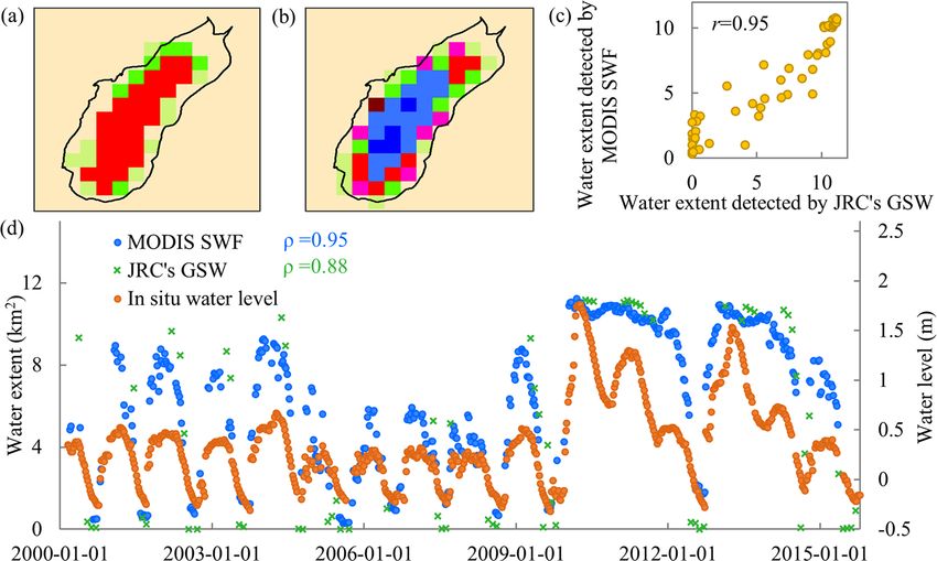
L. Li et al.: A new dense 18-year time series of surface water fraction estimates                                                3043

Figure 3. Diagram of our approach for deriving the surface water fraction.

members’ predictions are averaged to give a final prediction            4.1.4   Mapping and post-processing
(Quinlan, 1993). The second parameter is “neighbors” and
allows the Cubist model to group similar samples in terms
of predictor variable values, and determine the average pre-            We applied the resulting model to the MCD43A4 V006 data
diction of these training samples (Kuhn et al., 2012; Quin-             from February 2000 to December 2017 to produce gridded
lan, 1993). We tuned the models over different values of                time series of surface water fraction for the Mediterranean
“committees” and “neighbors” (“committees” was set to be                region with an 8 d time step resulting in 46 maps per year
0, 10 , 20, 50, and 100, and “neighbors” was set to be 0, 1,            (except for 2000, which only contained 39 images).
5, and 9) through a 10-fold cross-validation on our training               Recent studies on surface water detection using opti-
data and selected the values that produced the smallest root            cal sensors showed that multiple sources of commission
mean square error (RMSE).                                               errors exist, such as terrain and building shadows (Klein
   The resulting model was evaluated on both the training               et al., 2017; Pekel et al., 2016). These errors can be ac-
data that were used to generate the model and the inde-                 counted for using masks derived from auxiliary data (Klein
pendent validation data (Sect. 4.1.2). Three statistical mea-           et al., 2017; Pekel et al., 2016). In this study we addressed
sures were used to assess model performance: the coefficient            two sources of commission errors: shadows from buildings
of determination (R 2 ), mean absolute error (MAE), and the             and identified surface water presence that is unlikely on slop-
RMSE.                                                                   ing terrain. Specifically, a slope map was derived from the
                                                                        SRTM DEM by calculating the maximum rate of change in
                                                                        elevation from each raster cell to their eight neighbors. We
                                                                        then used a threshold of 5◦ to identify steep locations where
                                                                        it is unlikely to find surface water but could have been de-

www.hydrol-earth-syst-sci.net/23/3037/2019/                                          Hydrol. Earth Syst. Sci., 23, 3037–3056, 2019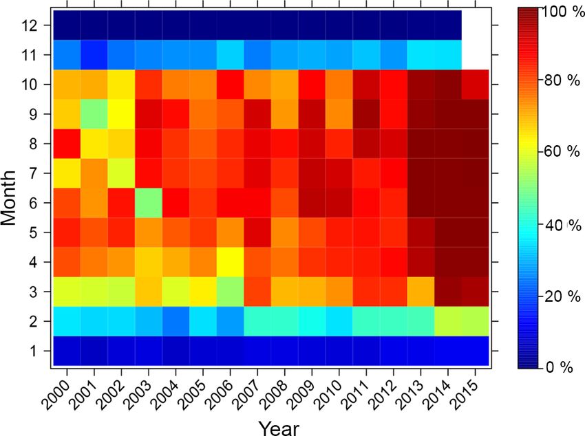
3044                                              L. Li et al.: A new dense 18-year time series of surface water fraction estimates

Table 2. Overview of the predictor variables used in this study. MODIS shortwave infrared bands are referred to as SWIR1 (1230–1250 nm),
SWIR2 (1628–1652 nm), and SWIR3 (2105–2155 nm).

 Predictor variable                     Formula                                                                  Reference
 MODIS individual bands (red, NIR,      –                                                                        –
 blue, green, SWIR1 , SWIR2 , and
 SWIR3 )
 NDVI – normalized difference vege-     (NIR − red) / (NIR + red)                                                Tucker (1979)
 tation index
 NDWI – normalized difference water     (green − NIR) / (green + NIR)                                            McFeeters (1996)
 index
 MNDWI – modified normalized dif-       (green − SWIR2 ) / (green + SWIR2 )                                      Xu (2006)
 ference water index
 NDWI – normalized difference water     (NIR − SWIR1 ) / (NIR + SWIR1 )                                          Gao (1996)
 index (referred as LSWIB5 )
 LSWI – land surface water index (re-   (NIR − SWIR2 ) / (NIR + SWIR2 )                                          Xiao et al. (2002)
 ferred as LSWIB6 )
 TCWI – tasseled cap wetness index      0.10839· red + 0.0912 · NIR + 0.5065 · blue + 0.404 · green −0.241       Zhang et al. (2002)
                                        · SWIR1 − 0.4658 · SWIR2 − 0.5306 · SWIR3
 TCBI – tasseled cap brightness index   0.3956 · red + 0.4718 · NIR + 0.3354 · blue + 0.3834                     Zhang et al. (2002)
                                        · green + 0.3946 · SWIR1 + 0.3434 · SWIR2 + 0.2964 · SWIR3
 Value (HSV)                            max(SWIR2 , NIR, red)                                                    Pekel et al. (2014)
 Saturation (HSV)                       1 − min(SWIR2 , NIR, red)/max(SWIR2 , NIR, red)                          Pekel et al. (2014)

                                            0, if V = min(SWIR2 , NIR, red)

                                                   60◦ ×(NIR−red)

                                                                            ◦       ◦
                                                V −min(SWIR2 ,NIR,red) + 360 mod 360 , if V = SWIR2
 Hue (HSV)                                                                                                       Pekel et al. (2014)
                                               60◦ ×(red−SWIR2 )         ◦
                                            V −min(SWIR2 ,NIR, red) + 120 , if V = NIR

                                              60◦ ×(SWIR2 −NIR)          ◦
                                            V −min(SWIR2 ,NIR, red) + 240 , if V = red

 TWI – topographic wetness index        ln(α/ tan β); α is the upslope area per unit contour length (m), which   Beven and Kirkby (1979)
                                        is calculated as (flow accumulation + 1) × (cell size); β is the slope
                                        expressed in radians

tected as water by our model, for example, due to spectral               4.2   Generation of the surface water fraction metrics
confusion between water and terrain shadows (Yamazaki et                       and comparison of products
al., 2015). In the case of building shadows, we used the ur-
ban class of the MODIS classification product MCD12Q1
                                                                         Based on gridded time series of surface water fraction, we
(Friedl et al., 2010) to assign areas potentially affected by
                                                                         derived a series of ecologically relevant metrics that capture
building-induced shadows. Pixels were reassigned to the 0 %
                                                                         both the intra- and inter-annual variability and changes, and
water fraction for slopes steeper than 5◦ and for areas clas-
                                                                         further compared these metrics with GSW-derived thematic
sified as urban in MCD12Q1, except for places where water
                                                                         products. The readily available GSW thematic products were
was present according to the GSW maximum water extent.
                                                                         derived from 32 years of data (between March 1984 and Oc-
                                                                         tober 2015); thus, they cannot be directly compared against
                                                                         our MODIS-based results for 2000–2017. Therefore, we re-
                                                                         produced the GSW thematic maps using the GSW monthly
                                                                         water history dataset from the overlapping period of these
                                                                         two datasets (i.e., February 2000–October 2015). We then

Hydrol. Earth Syst. Sci., 23, 3037–3056, 2019                                            www.hydrol-earth-syst-sci.net/23/3037/2019/
L. Li et al.: A new dense 18-year time series of surface water fraction estimates 3045
Table 3. Seasonality classification criteria based on surface water fraction and occurrence. The occurrence indicates how often the specified
surface water fraction is reached for a single hydrological year (October 2014–September 2015).
Class name Surface water fraction Water occurrence
Permanent water ≥ 70 % ≥ 90 %
Semipermanent water ≥ 70 % 70 %–90 %
Intermittent water ≥ 70 % 20 %–70 %
Infrequent inundation ≥ 70 % 1 %–20 %
Mixed permanent and semipermanent water 30 %–70 % ≥ 70 %
Mixed intermittent water 30 %–70 % 20 %–70 %
Mixed infrequent inundation 30 %–70 % 1 %–20 %
Never inundated < 30 % ≥ 0%
also computed the MODIS-derived temporal metrics for this present relative to the total valid observations (i.e., not
period. In total, 189 GSW water history images and 720 sur- affected by clouds). We adopted the classification crite-
face water fraction maps were incorporated for the gener- ria of Guerschmann et al. (2011) and further modified it
ation of these thematic maps. The following metrics were to be applicable to the Mediterranean region (Table 3).
generated: As the classes are not mutually exclusive, they are pri-
oritized in the order shown in Table 3.
1. The annual maximum and mean annual maximum sur-
face water fraction between 2000 and 2015: the GSW 4.3 Demonstrating the representation of surface water
monthly water history maps were summarized for each dynamics by the new MODIS dataset
year in GEE to calculate the annual maximum surface
water extent. We then aggregated the results of each To assess the performance of our MODIS-derived product
year to the MODIS resolution and averaged all years for monitoring temporal variations in the surface water ex-
to derive the mean annual maximum surface water frac- tent, we selected three lakes with fluctuating water presence.
tion. To assess the spatial agreement of the mean annual These three sites have varying sizes, and different geographic
maximum surface water fraction derived from MODIS locations and temporal dynamics, and have also been listed in
and GSW, we calculated the surface water area (in km2 ) the International Conventions on Wetlands (known as Ram-
from the mean annual maximum surface water fraction sar) given their importance for staging and wintering water-
using a threshold continuum. Specifically, the surface fowl. The three sites are as follows:
water fraction was partitioned using nine threshold val-
1. The Fuente de Piedra lake, Spain, which is a shal-
ues set in 10 % increments from 0 % to 100 %. All pix-
low and saline lake, has a maximum area of 13.6 km2 .
els with a surface water fraction greater than or equal to
It experiences strong seasonal, inter-annual, and intra-
the threshold were summed and then multiplied by the
annual variations of water level and inundation extent
MODIS pixel size. We then compared the water area
(Li et al., 2015).
(in km2 ) derived from the mean annual maximum sur-
face water fraction based on GSW and MODIS across a 2. Lake Sabkhat al-Jabbul, Syria, which is a large, perma-
different continuum of threshold values. We also com- nent saline lake that is surrounded by semiarid steppe.
pared the water area with the 250 m static water mask At high water levels, it contains two islands; it tradi-
from MOD44W. tionally floods in the spring and shrinks back during the
summer and autumn but seldom dries out completely
2. The standard deviation of the annual maximum: a mea-
(JAES-CC, 2010).
sure of the inter-annual variability of water presence.
3. The coastal marshland complex of Doñana, Spain,
3. The seasonality: a measure for the seasonal and intra-
which is separated from the ocean by an extensive dune
annual variability of water presence. We calculated the
system and is subject to seasonal and inter-annual vari-
number of times (i.e., the water occurrence) a given
ations in water level (De Castro and Reinoso, 1997).
pixel displayed standing water above a certain water
fractional threshold for a single hydrological year (Oc- For the first two lakes, we compared the time series of the
tober 2014 to September 2015), as GSW has a rela- MODIS-derived surface water area with that from GSW, and
tively large number of valid observations for this year further compared these against water level data from satellite
(Fig. 2), and then classified different types of water per- altimetry or in situ measurements. We calculated the Spear-
manence. The water occurrence was calculated for each man rank correlation (ρ) between water level and water area
grid cell as a fraction of the number of times water was derived from MODIS SWF and JRC’s GSW data to assess
www.hydrol-earth-syst-sci.net/23/3037/2019/ Hydrol. Earth Syst. Sci., 23, 3037–3056, 20193046 L. Li et al.: A new dense 18-year time series of surface water fraction estimates
Table 4. Statistical measures between the predicted surface water (Fig. 4). These differences likely correspond to the presence
fraction and the actual data for training and validation data, and for of wet meadows, salt marshes, and floodplains along large
different types of water permanence using validation data. rivers, which are usually saturated and inundated with water
during most of the vegetative season (Šefferová Stanová et
R2 RMSE (%) MAE (%) al., 2008; Stefan et al., 2016). Around the Po River in Italy,
Training data 0.93 9.79 5.61 where rice paddies are seasonally present, our MODIS prod-
Validation data 0.91 11.41 6.39 uct also shows larger surface water fractions (Fig. 4c). This
result suggests that the MODIS-derived surface water frac-
Permanent water 0.90 12.07 6.38 tion has enhanced sensitivity to surface water in wetland ar-
Fluctuating water 0.85 12.60 8.11
eas with emerged vegetation, and this could be attributed to
the fact that several predictor variables such as LSWI (Xiao
et al., 2002) are also sensitive to vegetation water content
the correspondence between these datasets. For Doñana, we (Li et al., 2015). Table 5 confirms that the total surface wa-
compared the monthly spatial distribution of the surface wa- ter areas for the Mediterranean calculated from MODIS are
ter extent derived from MODIS and JRC’s GSW. To ensure more comparable to the GSW results when only consider-
the accuracy of the area calculations, we only calculated an ing areas with a higher surface water fraction. For exam-
area for times when it contained at least 95 % of valid data ple, when only accounting for pixels with surface water frac-
from MODIS SWF and JRC’s GSW data. tions equal to or greater than 50 %, the total surface water
areas for the Mediterranean based on both datasets are simi-
lar (75 107 km2 for GSW versus 73 444 km2 for MODIS). In
5 Results
comparison, only 70 543 km2 of water was detected in this
region based on the 250 m static water mask from MOD44W.
5.1 Model performance
This implies that our MODIS product detects more surface
Following the model tuning of the Cubist regression model water than other coarse-resolution binary maps. Nonetheless,
(see Sect. 4.1.3), we found that a 20-member committee and our MODIS product detects less surface water than GSW
9-neighbor model resulted in the smallest RMSE between the for larger thresholds (≥ 50 %), whereas it detects much more
actual (GSW-derived) water fraction and our MODIS-based surface water than GSW for small thresholds (≤ 20 %). This
water fraction estimates. The addition of more committees or confirms an earlier finding that machine learning approaches
neighbors had little effect on the accuracy. such as Cubist and random forest often underestimate large
Table 4 shows the statistical measures between the pre- values and overestimate small values when estimating the
dicted and actual surface water fraction. The model predicted fractional cover of land surface (e.g., Huang et al., 2014; Li
surface water fraction shows good agreement with the actual et al., 2018; Wang et al., 2017). In addition to the effects
value with an R 2 of 0.93 for the training data. When testing of mixed pixels (Klein et al., 2017), the most obvious rea-
using the independent validation dataset, the R 2 value is only son for this is because regression techniques used in such
slightly smaller, and the RMSE and MAE are slightly larger, approaches fit linear equations to relationships that may not
suggesting that the Cubist regression model does not suffer be linear over the entire range of values.
from overfitting. The RMSE and MAE for fluctuating water Figure 5 shows the standard deviation of the annual maxi-
were slightly larger than for permanent water (Table 4). This mum surface water fraction. It indicates that areas of large
suggests that the developed model not only provides accu- inter-annual variability agree between MODIS-based and
rate results for the static mapping of the surface water frac- GSW-based results. Both indicate a larger variability in the
tion, but it can also be applied effectively for monitoring the surface water fraction in semiarid and desert climate zones,
dynamics of fluctuating surface water. particularly in the north of Algeria, for the Volga Delta in
the Caspian depression, and along the Tigris and Euphrates
5.2 Surface water fraction metrics and comparison of rivers of Iraq.
products Figure 6 displays the seasonality metric for the entire study
area, with details for two selected sites shown in panels (a)
The mean annual maximum surface water fraction values and (b) of Figs. 7 and 8. Fuente de Piedra is a seasonally
generated from GSW and the MODIS-derived product over flooded lake which usually dries out completely in summer
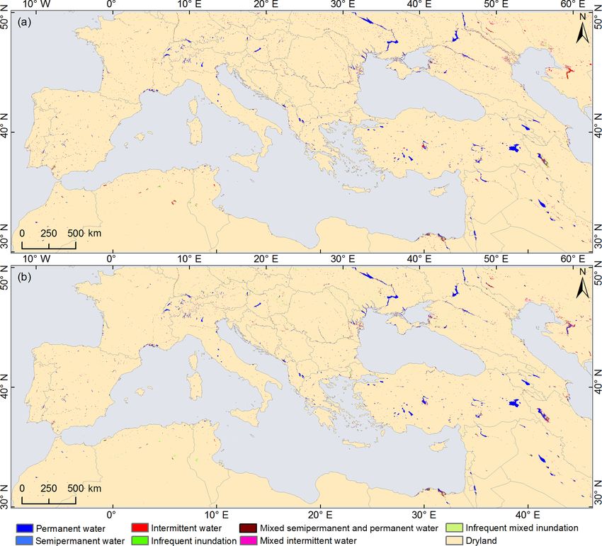
the 2000–2015 period are displayed in Fig. 4. Overall, the (May–September) (Batanero et al., 2017; Li et al., 2015) with
two maps are in good agreement. Visual comparison indi- the exception of extremely wet years (e.g., 2010, 2011, 2013:
cates that our MODIS-derived product is able to detect nar- Rodriguez-Rodriguez et al., 2016) when water was present
row rivers with widths covering a couple of MODIS pixels, throughout the whole year. The differences in water seasonal-
such as the Danube, Euphrates, Po, Rhine, and Tagus rivers. ity for Fuente de Piedra between the two products (Fig. 7a, b)
Large differences are evident for some low surface water can be attributed to the fact that GSW lacks observations in
fraction regions such as parts of Hungary and the Ukraine wet seasons, resulting in a reduced water occurrence com-
Hydrol. Earth Syst. Sci., 23, 3037–3056, 2019 www.hydrol-earth-syst-sci.net/23/3037/2019/L. Li et al.: A new dense 18-year time series of surface water fraction estimates 3047
Figure 4. Mean annual maximum surface water fraction maps as obtained from (a) JRC’s GSW and (b) MODIS time series surface water
fraction for the period from 2000 to 2015, and (c) the difference between the two maps. Positive difference values indicate that our MODIS
dataset detected a larger water fraction than JRC’s GSW.
pared with our MODIS product. The discontinuities in the 5.3 MODIS-derived surface water dynamics for
Landsat record between seasons can affect the accuracy of selected lakes
seasonality information, which has also been demonstrated
by Klein et al. (2017) and Pekel et al. (2016). Permanent
Panels (d) of Figs. 7–8 show the time series of the sur-
water is present in parts of Lake Sabkhat al-Jabbul, but the
face water extent detected by MODIS and GSW for two se-
larger central portion of the lake has highly dynamic inter-
lected lakes. Fuente de Piedra (Fig. 7d) experiences large
mittent water (Fig. 8). Mixed permanent and semipermanent
temporal variability in the surface water extent throughout
waters are mostly found on the edge of permanent water and
the year, which is well represented by our MODIS prod-
in narrow rivers.
uct with 461 time steps (Table 6). This variability corre-
sponds closely to the in situ water level data (ρ = 0.95). Note
that in extreme wet years (i.e., 2010, 2011, and 2013), the
lake remained flooded throughout the year without increas-
www.hydrol-earth-syst-sci.net/23/3037/2019/ Hydrol. Earth Syst. Sci., 23, 3037–3056, 20193048 L. Li et al.: A new dense 18-year time series of surface water fraction estimates
Table 5. Comparison of total surface water area (in km2 ) as determined from JRC’s GSW and MODIS mean annual maximum surface water
fraction maps for different thresholds.
Threshold for surface Total surface water areas Total surface water areas (km2 ) based on
water fraction (km2 ) based on GSW MODIS surface water fraction
90 % 48 718 47 145
80 % 55 887 51 778
70 % 62 371 58 996
60 % 68 855 65 993
50 % 75 107 73 444
40 % 81 220 82 417
30 % 87 217 96 239
20 % 93 207 142 531
10 % 99 260 284 916
Figure 5. Standard deviation of the surface water fraction as calculated from (a) JRC’s GSW and (b) MODIS annual maximum surface water
fraction maps for the period from 2000 to 2015.
Hydrol. Earth Syst. Sci., 23, 3037–3056, 2019 www.hydrol-earth-syst-sci.net/23/3037/2019/L. Li et al.: A new dense 18-year time series of surface water fraction estimates 3049 Figure 6. Seasonality information derived from time series of the (a) JRC’s GSW and (b) MODIS surface water fraction for a single year (October 2014 to September 2015). ing in size with regard to water level changes (Rodriguez- Table 6. Number of valid temporal observations for the three lakes Rodriguez et al., 2016). The water extent derived from based on the MODIS surface water fraction and JRC’s GSW be- MODIS SWF also matched closely to that from GSW tween February 2000 and October 2015. (Fig. 7c, d; r = 0.95). GSW only had 73 valid time steps with most observations in dry seasons (i.e., June to October); Lakes MODIS surface JRC’s thus, it did not allow for the appropriate capture of the sea- water fraction GSW sonal dynamics, particularly for the November–March period Fuente de Piedra 461 73 when the lake usually reaches its full surface water extent. Lake Sabkhat al-Jabbul 563 69 Time series of the water extent of Lake Sabkhat al-Jabbul as Doñana 714 70 determined by our MODIS product showed a relative high correlation with water level data (ρ = 0.69). It also showed good agreement with the water extent derived from GSW, in- cluding the seasonal peak extent and the minimum surface Figure 9 compares the MODIS monthly surface water water extent during the dry season (Fig. 8c, d; r = 0.88). fraction with the GSW monthly water history for Doñana, This implies that the coarse 500 m MODIS data not only pro- Spain. The visual comparison shows that the distribution of vide more detailed temporal information (563 MODIS sur- the MODIS surface water fraction agrees well with the GSW face water fraction time steps versus 69 GSW time steps) monthly water maps. The 500 m MODIS surface water frac- (Table 6), but they also give accurate estimations of the sur- tion is able to capture the spatial patterns as detected from the face water area compared with the results from Landsat 30 m high-resolution Landsat-based GSW dataset. Seasonal dry- resolution data. ing out and flooding of the wetland is well detected with the www.hydrol-earth-syst-sci.net/23/3037/2019/ Hydrol. Earth Syst. Sci., 23, 3037–3056, 2019
3050                                           L. Li et al.: A new dense 18-year time series of surface water fraction estimates

Figure 7. Seasonality information derived from (a) JRC’s GSW and (b) the MODIS surface water fraction from a single year (October 2014
to September 2015). The colors in (a) and (b) are the same as in Fig. 6. (c) A scatterplot of the water area obtained from JRC’s GSW versus
that from MODIS SWF. r represents the Pearson correlation between two datasets. (d) A comparison of time series of the surface water area
(in km2 ) derived from JRC’s GSW (shown using green asterisks) with MODIS surface water fraction (shown using blue dots) from 2000
to 2015, along with in situ water level data (shown using orange dots) for Fuente de Piedra, Spain. ρ represents the Spearman rank correlation
between the water level and water area.

Figure 8. As in Fig. 7, but for Lake Sabkhat al-Jabbul, Syria. The water level for this lake is computed from Jason-2/OSTM altimetry and
repeats every 10 d.

MODIS-derived surface water fraction, whereas GSW lacks                  6    Discussion
temporal details, for example, during large water extents in
November and December. MODIS also captures the timing
of the maximum water extent (i.e., in January) and water re-             We estimated the surface water fraction for the Mediter-
treat (i.e., in July). This example highlights that the infor-           ranean region from MODIS data, and improved on previ-
mation provided by our MODIS product can contribute to a                 ous efforts to estimate surface water fraction from medium-
better understanding of surface water dynamics.                          resolution imagery (MODIS or similar). The prediction ac-
                                                                         curacy of our model (R 2 = 0.91, RMSE = 11.41 %, and

Hydrol. Earth Syst. Sci., 23, 3037–3056, 2019                                           www.hydrol-earth-syst-sci.net/23/3037/2019/
L. Li et al.: A new dense 18-year time series of surface water fraction estimates 3051 Figure 9. Comparison of monthly water distribution based on (a) the Landsat-based GSW dataset and (b) the MODIS surface water fraction for Doñana, Spain, for 2011. MAE = 6.39 %) is higher than the R 2 of 0.625 reported over longer periods. The MODIS surface water fraction can by Weiss and Crabtree (2011), who used a linear regres- also accurately detect the spatial distribution of surface wa- sion model, and the R 2 of 0.7 reported by Guerschmann et ter inclusive of small water bodies (less than one MODIS al. (2011), using a logistic regression model. This research pixel) and narrow rivers, which are missing in other coarse- successfully expanded our previous work (Li et al., 2018) resolution products using binary classification method such by upscaling it from a relatively small region to the whole as MOD44W (Salomon et al., 2004). Metrics derived from Mediterranean while retaining a similar high accuracy (both the MODIS surface water fraction and GSW time series can achieved an R 2 of 0.91). This attributes to the feasibility reflect different facets of surface water dynamics. The accu- and robustness of Cubist regression modeling with respect to racy of some metrics, such as seasonality, relies on the num- dealing with different environmental conditions when train- ber of valid observations and the temporal interval. Landsat- ing data are collected across a wide geography resulting in derived metrics might be problematic in areas with large tem- varying spectral characteristics. poral gaps caused by persistent cloud cover, as shown in this Secondly, we generated surface water fraction maps at study (Fig. 8) and previously by Pekel et al. (2016) and Klein high temporal frequency, which is an advantage over ex- et al. (2017). Although cloud coverage also limits MODIS isting fine-resolution datasets. Our MODIS-derived surface observations, the probability of obtaining cloud-free obser- water fraction product accurately displays the spatiotempo- vations is higher (Table 6) due to the daily acquisitions and ral variability of surface water. The comparison with the consequent temporal compositing possibilities. With these GSW 30 m product and water level data (Figs. 7–9) reveal advantages, we expect that our MODIS surface water frac- that our product can efficiently monitor the seasonal, intra- tion product could fill in important information on surface annual, and long-term surface water dynamics with good water for areas and time periods for which cloud-free Land- spatial and temporal accuracy. For example, it complements sat acquisitions are few or non-existent. the GSW by allowing for the detection of inundation and re- Our MODIS-derived surface water fraction product also cession processes over short time periods and for the bet- has limitations. Firstly, it is designed to detect only open sur- ter representation of seasonality changes and temporal trends face water; therefore, it may not effectively capture water www.hydrol-earth-syst-sci.net/23/3037/2019/ Hydrol. Earth Syst. Sci., 23, 3037–3056, 2019
3052                                         L. Li et al.: A new dense 18-year time series of surface water fraction estimates

bodies covered by dense vegetation, such as swamps, lakes           newly formed and disappearing water bodies, and estimating
with considerable coverage of aquatic vegetation, and in-           global water loss. The MODIS surface water fraction dataset
undated dense forests. Secondly, the MODIS surface water            may help to improve the calibration and validation of hy-
fraction product overestimates small surface water fractions        drological models. For example, the water area can help to
of less than 20 % (Table 5), which has also been found in           estimate a series of hydrological parameters such as water
previous studies on surface water fraction mapping (Li et           discharge (Huang et al., 2018) and water volume (Busker et
al., 2018; Parrens et al., 2017). This overestimation might         al., 2019; Cael et al., 2017; Duan and Bastiaanssen, 2013;
be attributed to the mixed spectral response of pixels with         Tong et al., 2016). This would be particularly useful for ar-
different land cover types, as already demonstrated by many         eas where in situ measurements are sparse or inaccessible.
studies (e.g., Guerschmann et al., 2011; Klein et al., 2017).       Closely monitoring hydrological variability is important for
Further work could consider reassigning pixels with less            understanding how climate change, meteorological variabil-
than 20 % surface water to 0 % water fraction for locations         ity, and human activities affect the dynamics of surface water
where water is never present according to the GSW max-              and human livelihoods (Tulbure and Broich, 2019; Zhang et
imum water extent. Thirdly, the auxiliary layers utilized for       al., 2019). It may also provide new insights for understand-
the identification of potential areas of commission errors also     ing how surface water dynamics further influence climate.
appear to have some limitations. For example, some urban ar-        For example, lake expansion and the creation of new dams
eas might be not mapped in MCD12Q1, and areas of cloud              can alter local and regional precipitation patterns (Ekhtiari et
cover and cloud shadow might not be completely removed              al., 2017; Hossain et al., 2009; Mohamed Degu et al., 2011).
from the MCD43A4 product. The importance of these lim-              Similarly, our long-term records and derived metrics have the
itations may diminish as the quality of these auxiliary lay-        potential to contribute to the management and conservation
ers improves or dynamic datasets rather than static layers          of biodiversity and other ecosystem services associated with
are incorporated (e.g., Global Human Settlement Layer: Pe-          terrestrial surface water and wetlands.
saresi et al., 2016). Fourthly, the MCD43A4 product also suf-
fers from many missing values, especially in regions with
large amounts of precipitation, aerosol concentrations, or          7   Conclusion
snow and ice coverage (Klein et al., 2017). Future research
                                                                    We derived an 8 d, 500 m resolution surface water fraction
should focus on combining other moderate-resolution data
                                                                    product over the Mediterranean for the period from 2000
(e.g., MOD09) for areas with missing data to ensure a gap-
                                                                    to 2017 by applying a global Cubist regression tree model
free reconstruction of inland water development for the past
                                                                    to MODIS and SRTM data. We validated the results with
and future.
                                                                    JRC’s Landsat-derived GSW dataset, which resulted in a
   This work can be further scaled up over much larger re-
                                                                    high overall accuracy (R 2 = 0.91, RMSE = 11.41 %, and
gions and for shorter (e.g., daily) time intervals. A high-
                                                                    MAE = 6.39 %). The MODIS-derived surface water fraction
quality training dataset is crucial for the effective application
                                                                    showed a good spatial and temporal correspondence with
of the rule-base regression model and the collection of such
                                                                    JRC’s GSW. Comparison with satellite altimetry and in situ
training data is time consuming (Sun et al., 2012). In this pa-
                                                                    water level data for selected lakes demonstrated the ability
per, time series of the GSW monthly water history dataset
                                                                    of MODIS surface water fraction to effectively monitor sea-
proved to be an efficient basis for building a reliable train-
                                                                    sonal and inter-annual changes in surface water extent. Our
ing dataset. Considering that GSW is globally available, we
                                                                    dataset provides a consistent, long-term record (18 years) of
are confident that our approach can be scaled to monitor the
                                                                    8 d water fraction dynamics for the Mediterranean region,
surface water fraction globally with MODIS data. Although
                                                                    and complements fine spatial resolution surface water prod-
the surface water fraction maps were produced with an 8 d
                                                                    ucts, especially in regions where such products have long
time step, the model developed in this paper was actually
                                                                    temporal and spatial data gaps due to both the limited num-
trained using daily MODIS data and could be directly ap-
                                                                    ber of acquisitions and persistent cloud cover. Our approach
plied to that temporal resolution. The resulting daily surface
                                                                    is also promising for monitoring surface water fraction at the
water fraction maps could be of high interest for ecological
                                                                    global scale and at a daily interval.
and hydrological research. The recent GCOS report requires
water extent and lake ice cover with a daily temporal reso-
lution and a 20 m and 300 m spatial resolution, respectively
                                                                    Data availability. The final derived 18 years of surface water
(Belward, 2016). Our approach makes this requirement for            fraction maps for the Mediterranean region are available from
the coarser of the two resolutions within reach.                    https://doi.org/10.17026/dans-xrz-y92s (Li, 2019). The GEE and R
   Our MODIS surface water fraction dataset may benefit a           code used for this paper are available upon request from the first
large number of applications. For example, it could be used         author.
as a monitoring tool for analyzing hydrologic extremes such
as floods and droughts, detecting abnormal changes of wet-
land hydrology, capturing short-duration events, identifying

Hydrol. Earth Syst. Sci., 23, 3037–3056, 2019                                     www.hydrol-earth-syst-sci.net/23/3037/2019/
You can also read