A framework for deriving drought indicators from the Gravity Recovery and Climate Experiment (GRACE)
←
→
Page content transcription
If your browser does not render page correctly, please read the page content below
Hydrol. Earth Syst. Sci., 24, 227–248, 2020
https://doi.org/10.5194/hess-24-227-2020
© Author(s) 2020. This work is distributed under
the Creative Commons Attribution 4.0 License.

A framework for deriving drought indicators from the Gravity
Recovery and Climate Experiment (GRACE)
Helena Gerdener, Olga Engels, and Jürgen Kusche
Institute of Geodesy and Geoinformation, University of Bonn, Bonn, Germany

Correspondence: Helena Gerdener (gerdener@geod.uni-bonn.de)

Received: 28 May 2019 – Discussion started: 19 June 2019
Revised: 16 October 2019 – Accepted: 10 December 2019 – Published: 16 January 2020

Abstract. Identifying and quantifying drought in retrospec-        1   Introduction
tive is a necessity for better understanding drought conditions
and the propagation of drought through the hydrological cy-        Droughts are recurrent natural hazards that affect the envi-
cle and eventually for developing forecast systems. Hydro-         ronment and economy with potentially catastrophic conse-
logical droughts refer to water deficits in surface and subsur-    quences. Drought impacts range from reduced streamflow,
face storage, and since these are difficult to monitor at larger   water scarcity, and reduced water quality to increased wild-
scales, several studies have suggested exploiting total water      fires, soil erosion, and increased quantities of dust, crop fail-
storage data from the GRACE (Gravity Recovery and Cli-             ure, and large-scale famine. With climate change and pop-
mate Experiment) satellite gravity mission to analyze them.        ulation growth, the frequency and impact of droughts are
This has led to the development of GRACE-based drought             projected to increase for many regions of the world (IPCC,
indicators. However, it is unclear how the ubiquitous pres-        2013). Drought types can be distinguished depending on
ence of climate-related or anthropogenic water storage trends      their effect on the hydrological cycle (e.g., Changnon, 1987;
found within GRACE analyses masks drought signals. Thus,           Mishra and Singh, 2010). In this study we focus on hydro-
this study aims to better understand how drought signals           logical drought, a multiscale problem which may last weeks
propagate through GRACE drought indicators in the pres-            or many years and which may affect local or continental re-
ence of linear trends, constant accelerations, and GRACE-          gions. For example, the severe drought between mid-2011
specific spatial noise. Synthetic data are constructed and ex-     and mid-2012 affected millions of people in the entire east-
isting indicators are modified to possibly improve drought         ern Africa region (Somalia, Djibouti, Ethiopia, and Kenya)
detection. Our results indicate that while the choice of the       and led to famine with an estimated 258 000 deaths (Chec-
indicator should be application-dependent, large differences       chhi and Robinson, 2013). From 2012 to 2016, the US state
in robustness can be observed. We found a modified, tempo-         of California experienced a historical drought that adversely
rally accumulated version of the Zhao et al. (2017) indicator      affected groundwater levels, forests, crops, and fish popu-
particularly robust under realistic simulations. We show that      lations and led to widespread land subsidence (Mann and
linear trends and constant accelerations seen in GRACE data        Gleick, 2015; Moore et al., 2016). In contrast, European
tend to mask drought signals in indicators and that differ-        droughts, for example in 2018, typically last a few months in
ent spatial averaging methods required to suppress the spa-        exceptionally dry summers. For South Africa, due to a com-
tially correlated GRACE noise affect the outcome. Finally,         plex rainfall regime, areas and the percentage of land surface
we identify and analyze two droughts in South Africa using         affected by drought can vary strongly (Rouault and Richard,
real GRACE data and the modified indicators.                       2005).
                                                                      Hydrological drought refers to a deficit of accessible wa-
                                                                   ter, i.e., water in natural and man-made surface reservoirs and
                                                                   subsurface storage, with respect to normal conditions. The
                                                                   propagation of drought through the hydrological cycle typ-
                                                                   ically begins with a lack of precipitation, leading to runoff

Published by Copernicus Publications on behalf of the European Geosciences Union.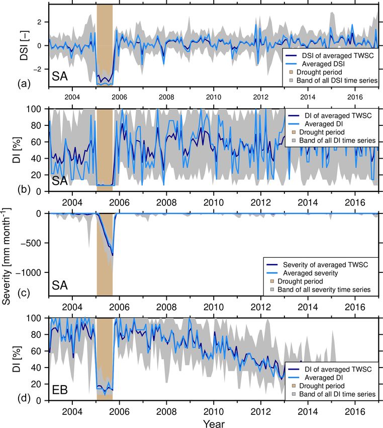
228                         H. Gerdener et al.: Gravity Recovery and Climate Experiment (GRACE) drought indicators

and soil moisture deficit, followed by decreasing stream-        separate different storage compartments, such as groundwa-
flow and groundwater levels (Changnon, 1987). However, no        ter storage, without utilizing additional (e.g., compartment-
unique standard procedures exist for measuring the deficit       specific) observations or model outputs, and their spatial
of each of these factors and for defining normal conditions.     and temporal resolutions (about 300 km and nominally 1
In order to arrive at operational definitions, which are re-     month respectively for GRACE) are limited. Several efforts
quired for triggering a response according to drought class      are therefore focused on assimilating GRACE-TWSC maps
for example, a large variety of drought indicators has been      into hydrological or land surface models (e.g., Zaitchik et al.,
defined which typically seek to extract certain sub-signals      2008; Eicker et al., 2014; Girotto et al., 2016; Springer,
from observable fields (Bachmair et al., 2016; Wilhite, 2016;    2019).
Mishra and Singh, 2010; Van Loon, 2015). Reviews of hy-             Thus, perhaps not surprisingly, a number of GRACE-
drological drought indicators are contained in Keyantash and     based drought indicators have been suggested (e.g., Houborg
Dracup (2002), Wilhite (2016), Mishra and Singh (2010),          et al., 2012; Thomas et al., 2014; Zhao et al., 2017), typi-
and Tsakiris (2017). Streamflow is the most frequently used      cally either based on normalization or percentile rank meth-
observable measurement in these studies.                         ods. However, a comprehensive comparison and assessment
   Drought detection is mostly restricted to single fluxes       of these indicators is still missing, particularly in the presence
(precipitation or streamflow) or storage (surface soil mois-     of (1) trend signals as picked up by GRACE in many regions
ture or reservoir levels) that are easy to measure. Much         that may reflect non-stationary “normal” conditions, (2) cor-
fewer measurements are available to assess water content in      related spatial noise that is related to the peculiar GRACE
deeper soil layers and groundwater storage deficit or the to-    orbital pattern, and (3) the inevitable spatial averaging ap-
tal of all storages. The NASA and German Aerospace Center        plied to GRACE, which results in smoothing out noise (Wahr
(DLR) Gravity Recovery and Climate Experiment (GRACE)            et al., 1998). From a water balance perspective, GRACE-
satellite mission, launched in 2002, has changed this situ-      TWSC variability mainly represents monthly total precipita-
ation since GRACE-derived monthly gravity field models           tion anomalies (e.g., Chen et al., 2010; Frappart et al., 2013).
can be converted to total water storage changes (TWSCs;          It is thus obvious that GRACE drought indicators will con-
Wahr et al., 1998). GRACE consisted of two spacecraft fol-       tain signatures that are visible in meteorological drought in-
lowing each other, which were linked together by an ultra-       dicators, yet the difference should explain the magnitude of
precise microwave ranging instrument; these ranges are rou-      other contributions (e.g., increased evapotranspiration due to
tinely processed to provide monthly gravity models and thus      radiation) to hydrological drought.
maps of mass change. Since other mass transports in the             Figure 1 shows a time series of region-averaged, detrended
atmosphere and ocean are removed during the processing,          and deseasoned GRACE water storage changes over east-
GRACE indeed provides quantitative measure of surface and        ern Brazil (Ceará state) compared to the region-averaged
subsurface water storages (Chen et al., 2009; Frappart et al.,   6-month Standardized Precipitation Index (SPI) (McKee
2013). Meanwhile, GRACE has been continued with the              et al., 1993) to illustrate the potential of GRACE-TWSC for
GRACE-FO (Follow-On) mission from which the first data           drought monitoring. As can be expected, TWSC and 6-month
are now available.                                               SPI appear moderately similar (correlation 0.43), character-
   Studies of drought detection with GRACE-TWSC can              ized by positive peaks, for example at the beginning of 2004
be summarized in three groups: (i) using monthly maps of         and at the end of 2009, and negative peaks at the beginning
TWSC directly, (ii) partitioning TWSC time series into sub-      of 2013. We also found correlations between TWSC and
signals that include drought signatures, or (iii) using in-      6-month SPI in regions with different hydro-climatic con-
dicators. For example, Seitz et al. (2008) investigated the      ditions for the Missouri river basin (0.31), Maharashtra in
2003 heat wave over seven central European basins using          western India (0.46), and South Africa (0.45) among other
GRACE time series; they found a good agreement between           regions. This motivates us to modify common GRACE in-
TWSC and the combination of net precipitation and evap-          dicators to account for accumulation periods of input data,
oration. Other studies focused on drought detection using        e.g., used with 6-month SPI but also for periods that are
TWSC sub-signals, e.g., trends were used to identify drought     based on differences of input data. To our knowledge, this
in central Europe (Andersen et al., 2005) and for the region     is the first study where (modified) indicators are tested in a
encompassing the Tigris, Euphrates, and western Iran (Voss       synthetic framework based on a realistic signal that includes
et al., 2013). After decomposing GRACE-TWSC into a sea-          a hypothetical drought. We hypothesize that in this way we
sonal and non-seasonal signals, Chen et al. (2009) were able     can (i) assess indicator robustness, with respect to identifying
to detect the 2005 drought in the central Amazon river basin     a “true” drought of given duration and magnitude, and (ii) un-
while, Zhang et al. (2015) identified two droughts in 2006       derstand how trend signals and spatial noise propagate into
and 2011 in the Yangtze river basin. In the latter study, the    indicators and mask drought detection. In addition, we in-
El Niño–Southern Oscillation (ENSO) was identified as a          vestigate to what extent the spatial averaging that is required
possible driver for drought events in the Yangtze river basin.   for analyzing GRACE data affects indicators. For this, we
However, neither GRACE nor GRACE-FO enable one to

Hydrol. Earth Syst. Sci., 24, 227–248, 2020                                     www.hydrol-earth-syst-sci.net/24/227/2020/
H. Gerdener et al.: Gravity Recovery and Climate Experiment (GRACE) drought indicators                                               229

                                                                   monthly GRACE data without any additional information.
                                                                   Therefore, these three indicators will be discussed further.
                                                                      In order to stress the link between GRACE-based and
                                                                   meteorological indicators, we first describe the relation of
                                                                   TWSC and precipitation. Assuming evapotranspiration (E)
                                                                   and runoff (Q) vary more regularly as compared to precip-
                                                                   itation (i.e., 1E = 0 and 1Q = 0), the monthly GRACE-
                                                                   TWSC (1s) corresponds to precipitation anomalies (1P )
                                                                   accumulated since the GRACE storage monitoring began.
                                                                                   t
                                                                                   X
Figure 1. Detrended and deseasoned GRACE-TWSC [mm] (or-            1s(t) = 1t           1P ,                                         (1)
ange) and the SPI [–] for 6 months of accumulated precipitation                    t0
(blue), spatially averaged for Ceará, Brazil.                      where 1t is the time from t0 to t1 . In contrast to Eq. (1), the
                                                                   difference between GRACE months as in
                                                                                            t2
                                                                                            X
compare spatially averaged gridded indicators to indicators        1s (t2 ) − 1s (t1 ) = 1t    1P ,                             (2)
derived from spatially averaged TWSC.                                                              t1
   This contribution is organized as follows: in Sect. 2 we        which corresponds to the precipitation anomaly accumulated
will review three GRACE-based drought indicators and mod-          between these months. Accumulated monthly TWSC thus
ify them to accommodate either multi-month accumulation            corresponds to an iterative summation over the precipitation
or differencing, while in Sect. 3 our framework for testing        anomalies described by
GRACE indicators in a realistic simulation environment will
                                                                   t                    t X
                                                                                          τ
be explained. Then, Sect. 4 will provide simulation results        X
                                                                          1s(t) = 1t
                                                                                        X
                                                                                                   1P .                              (3)
and finally the results from real GRACE data. A discussion          t0                  τ =t0 t0
and conclusion will complete the paper.
                                                                   In the following, we will discuss and extend the definition of
                                                                   Zhao et al. (2017), Houborg et al. (2012), and Thomas et al.
                                                                   (2014) GRACE-based indicators, which are hence referred to
2   Indicators for hydrological drought                            as the Zhao method, Houborg method, and Thomas method,
                                                                   respectively.
Hydrological drought indicators are mostly based on obser-
vations of single water storages or fluxes, e.g., for precipita-   2.1     Zhao method
tion, snowpack, streamflow, or groundwater. In general, indi-
cator definitions can be arranged into four categories: (1) data   In the approach of Zhao et al. (2017), one considers GRACE-
normalization, (2) threshold-based, (3) quantile scores, and       derived monthly gridded TWSC for n years as in
(4) probability-based (e.g., Zargar et al., 2011; Keyantash

                                                                   xi,j = 1s ti,j ,                                         (4)
and Dracup, 2002; Tsakiris, 2017).
   Since total water storage deficit may be viewed as a more       with

comprehensive information source on drought, the advent of                       1             1
                                                                   ti,j   =i+ j−                 i = 1, . . ., n j = 1, . . ., 12.   (5)
GRACE total water storage change data has led to new indi-                       2            12
cators being developed. For example, Frappart et al. (2013)        Let us define the monthly climatology, i.e., mean monthly
developed a drought indicator based on yearly minima of            TWSC, x̃j with j = 1, . . . , 12 and the standard deviation σ̃j
water storage and a method for standardization, and Kusche         of the anomalies in month j with respect to the climatologi-
et al. (2016) computed recurrence times of yearly minima           cal value as
through the generalized extreme value theory. Other indica-                 n
tors explore the monthly resolution of GRACE, e.g., the To-              1X
                                                                   x̃j =       xi,j ,                                         (6)
tal Storage Deficit Index (TSDI; Agboma et al., 2009), the               n i=1
GRACE-based Hydrological Drought Index (GHDI; Yi and                                            !1/2
                                                                              n
Wen, 2016), the Drought Severity Index (DSI; Zhao et al.,                  1X                2
                                                                   σ̃j =          xi,j − x̃j         .                        (7)
2017), and the drought index (DI; Houborg et al., 2012). Fur-              n i=1
ther, Thomas et al. (2014) presented a water storage deficit
approach to detect drought magnitude, duration, and severity       Zhao et al. (2017) define their drought severity index
based on GRACE-derived TWSC. To our knowledge, only                (GRACE-DSI) as the standardized anomaly
the Zhao et al. (2017), Houborg et al. (2012), and Thomas                                 xi,j − x̃j
                                                                   TWSC-DSIi,j =                                                     (8)
et al. (2014) methods are able to detect drought events from                                  σ̃j

www.hydrol-earth-syst-sci.net/24/227/2020/                                              Hydrol. Earth Syst. Sci., 24, 227–248, 2020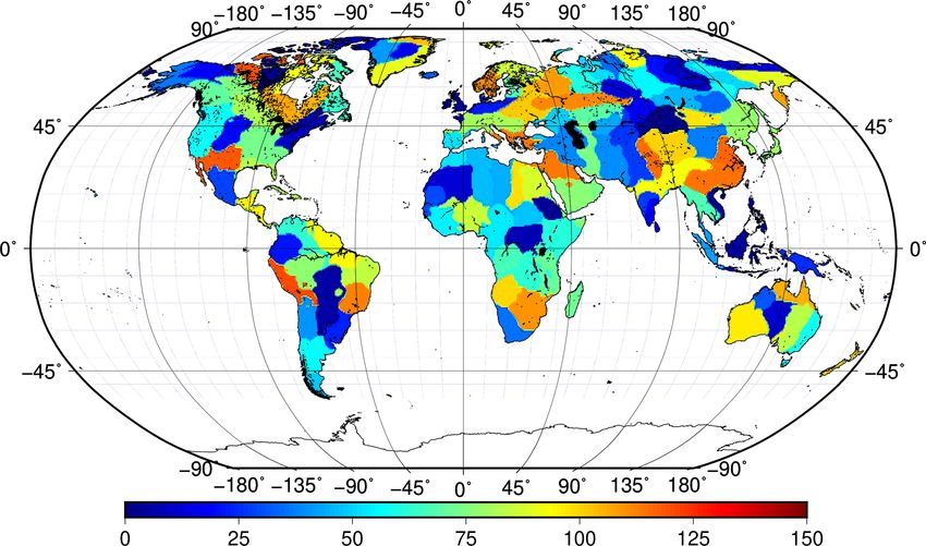
230                               H. Gerdener et al.: Gravity Recovery and Climate Experiment (GRACE) drought indicators

Table 1. Drought severity level of TWSC-DSI (Zhao et al., 2017).   Table 2. Drought severity level of TWSC-DI (Houborg et al., 2012).
The values of TWSC-DSI are unitless.                               The values of TWSC-DI are given in %.

                                          TWSC-DSI [–]                                                         TWSC-DI [%]
                 Drought severity level   Min.   Max.                           Drought severity level         Min.   Max.
                 Abnormal                 −0.8   −0.5                           Abnormal                        20      30
                 Moderate                 −1.3   −0.8                           Moderate                        10      20
                 Severe                   −1.6   −1.3                           Severe                           5      10
                 Extreme                  −2.0   −1.6                           Extreme                          2       5
                 Exceptional                     −2.0                           Exceptional                      0       2

of a given month ti,j and provide a scale from −2.0 (ex-
ceptional drought) to +2.0 (exceptionally wet), as shown in                               +
                                                                                         xi,j,q     +
                                                                                                − x̃j,q
Table 1. There is no particular probability distribution func-     TWSC-DSIAi,j,q =             +                               (12)
tion (PDF) underlying the method; however if we assume                                        σ̃j,q
the anomalies for a given month follow a Gaussian PDF, it is
straightforward to compute the likelihood of a given month         and
falling in one of the Zhao et al. (2017) severity classes. For                             −
                                                                                          xi,j,q     −
                                                                                                 − x̃j,q
example, 2.1 % of months would be expected to turn out to          TWSA-DSIDi,j,q =             −          .                    (13)
be a period of exceptional drought and 2.1 % as exceptionally                                 σ̃j,q
wet. This can be applied to any other PDF.
                                                                   Finally, it is obvious that sampling the full climatological
   Drought severity, however, should be related to the dura-
                                                                   range of dry and wet months is not yet possible with the lim-
tion of a drought. For example McKee et al. (1993) showed
                                                                   ited GRACE data period. Therefore, Zhao et al. (2017) sug-
how typical time scales of 3, 6, 12, 24, and 48 months of pre-
                                                                   gest applying a bias correction to avoid the under- or overes-
cipitation deficits are related to their impact on usable wa-
                                                                   timation of drought events. This implies using TWSC from
ter sources. To account for the relation between severity and
                                                                   multi-decadal model runs, which is feasible but is not the fo-
duration in the Zhao et al. (2017) approach, we consider q
                                                                   cus of this study.
months accumulated of TWSC, which is approximately re-
lated to precipitation in Eq. (3) as                               2.2   Houborg method
           q
           X
 +
                                                                   Houborg et al. (2012) define the drought indicator GRACE-
xi,j,q =         1s ti,j +1−q ,                             (9)
           k=1                                                     DI via the percentile of a given month, ti,j , with respect to
                                                                   the cumulative distribution function (CDF). The GRACE-DI
with ti,j +1−q = ti−1,j +13−q for j + 1 − q < 1 or equivalently
                                                                   is applied to TWSC by
written for q months of averaged TWSC as
                                                                                   P
                 q                                                                     xj ≤ xi,j
 +         1X
                                                                                    i
xi,j,q =         1s ti,j +1−q .                            (10)    TWSC-DIi,j =                    · 100,                   (14)
           q k=1                                                                        P
                                                                                          xj
                                                                                          i
For example for q = 3, we would look for the 3-month
running mean for December–January–February, January–               i.e., all years containing month j are counted for which
February–March, and so on. In the next step, one computes,         TWSC is equal or lower than TWSC in month j and year i,
for example, the climatology and anomalies as with the orig-       and these are normalized by the number of years that con-
inal method. On the other hand, we can relate hydrological to      tain month j . The indicator value is assigned to five sever-
meteorological indicators using Eq. (2). To develop a TWSC         ity classes as shown in Table 2. For example, exceptional
indicator that can be compared to indicators based on ac-          droughts occur up to 2 % of the entire time period at any
cumulated precipitation, one should rather consider the q-         location.
month differenced TWSC                                                Again, to relate drought severity to duration, we pro-
                                                                   ceed via multi-month accumulation (Eq. 9) and differences
  −
xi,j,q = 1s ti,j − 1s ti,j +1−q .                       (11)       (Eq. 11) resulting in the definition of two new indicators
                                                                   based on TWSC-DIi,j in Eq. (14),
Thus, as with TWSC-DSIi,j in Eq. (8), we can define
two new multi-month indicators (TWSC-DSIA and TWSC-
DSID) through standardization by using accumulated (A)
and differenced (D) TWSC (Eqs. 9 and 11) as

Hydrol. Earth Syst. Sci., 24, 227–248, 2020                                       www.hydrol-earth-syst-sci.net/24/227/2020/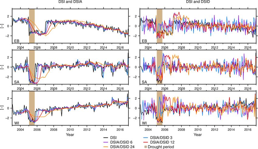
H. Gerdener et al.: Gravity Recovery and Climate Experiment (GRACE) drought indicators                                          231

                                                                    the duration di,j , the severity si,j of the drought event can
                     P    +      +

                          xj,q ≤ xi,j,q                             finally be computed by
                      i
TWSC-DIAi,j,q =                  +            · 100,        (15)
                                                                    si,j = 1xi,j di,j .                                        (19)
                           P
                                xj,q
                            i
                     P                                             Severity is therefore a measure of the combined impact of

                           −      −
                          xj,q ≤ xi,j,q
                      i                                             duration and magnitude of water storage deficit (see Thomas
TWSC-DIDi,j,q =            P     −            · 100.        (16)    et al., 2014; Humphrey et al., 2016).
                                xj,q
                            i

Assuming again that the CDF equals the cumulative Gaus-             3     Framework to derive synthetic TWSC for computing
sian PDF, 0.6 % of the months would be detected as ex-                    drought indicators
ceptionally dry and 9.5 % of the months as abnormally dry.
Houborg et al. (2012) applied the percentile approach sepa-         3.1    Methods
rately to surface soil moisture, root zone soil moisture, and
groundwater storage, which were derived by assimilating             In order to analyze the performance of drought indicators,
GRACE-derived TWSC into a hydrological model, and the               we first construct a synthetic time series of “true” total water
CDFs were adjusted to a long-term model run. Here, we fo-           storage changes on a grid. We base our drought simulations
cus on a simulated TWSC environment for the GRACE pe-               on the GRACE data model
riod only, and, as explained in Sect. 2.1, we therefore disre-
gard the bias correction.                                           1s(t) = x(t) + η(t) + (t),                                (20)

2.3   Thomas method                                                 including the introduced (in Sect. 2.3) signal x (which con-
                                                                    tains seasonality and a constant, linear, and time-varying
Thomas et al. (2014) define a drought by considering the            trend; Eq. 18), an interannual signal η (which has been de-
number of consecutive months below a threshold of TWSC.             trended and deseasoned and which will carry the simulated
Given TWSC observations xi,j and a threshold c, we can              true drought signature), and a GRACE-specific noise term .
compute anomalies by                                                To simulate the true signal as realistically as possible using
                                                                   Eq. (20), we first analyze real GRACE-TWSC data follow-
          0          for xi,j ≥ c                                   ing the steps summarized in Fig. 2. We derive (1) the sig-
1xi,j =                           .                 (17)
          xi,j − xj for xi,j < c.                                   nal components, constant, trend, acceleration, annual, and
While the threshold can be derived from different concepts,         semi-annual sine wave, (2) temporal correlations, (3) a repre-
Thomas et al. (2014) use the monthly climatology xj (Eq. 6).        sentative drought signal quantified by strength and duration,
Here, we also consider using a fitted signal for defining the       and (4) spatially correlated noise from GRACE error covari-
threshold. The signal is computed by                                ance matrices. While the first three steps are generic and can
                                                                    be used for simulating other observables, step 4 is directly
                             1                                      related to the measurement noise (in this case the GRACE
x(t) = a0 + a1 (t − t0 ) + a2 (t − t0 )2 + b1 cos(ωt)
                             2                                      noise).
     + b2 sin(ωt) + c1 cos(2ωt) + c2 sin(2ωt),              (18)       As an input to the simulation, GRACE-TWSC data are de-
                                                                    rived by mapping monthly ITSG-GRACE2016 gravity field
with time t with a constant a0 , a linear trend term a1 , a con-    solutions of degree and order 60, provided by the Graz Uni-
stant acceleration term a2 , annual signal terms b1 and b2 , and    versity of Technology (Mayer-Gürr et al., 2016), to TWSC
similarly semi-annual signal terms c1 and c2 . Trends and pos-      grids. As per standard practice, we add degree-1 spheri-
sible accelerations in GRACE-TWSC can result from many              cal harmonic coefficients from Swenson et al. (2008) and
different hydrological processes. For example, accelerations        degree 2, order 0 coefficients from laser ranging solutions
can result from trends in the flux precipitation, evapotranspi-     (Cheng et al., 2011). Then, we remove the temporal mean
ration, and runoff (e.g., Eicker et al., 2016). In the following,   field, apply DDK3 filtering (Kusche et al., 2009) to suppress
the linear trends are denoted as trends, and constant accelera-     excessive noise, and map coefficients to TWSC via spherical
tions are denoted as accelerations. The Thomas method then          harmonic synthesis. We also remove the effect of ongoing
identifies drought events through the computation of their          glacial isostatic adjustment (GIA) following A et al. (2013).
magnitude, duration, and severity: the magnitude or water              Droughts are a multiscale phenomenon, and for a realis-
storage deficit is equal to 1xi,j (Eq. 17), and the duration di,j   tic simulation we must first define the largest spatial scale to
is given by the number of consecutive months where TWSC             which we will apply the model of Eq. (20). In other words,
is below the threshold. Thomas et al. (2014) propose a mini-        we first need to identify coherent regions in the input data
mum number of 3 consecutive months required for the com-            for which our approach is then applied at the grid scale prior
putation of drought duration. By using the deficit 1xi,j and        to step 1. For this, we apply two consecutive steps: we first

www.hydrol-earth-syst-sci.net/24/227/2020/                                           Hydrol. Earth Syst. Sci., 24, 227–248, 2020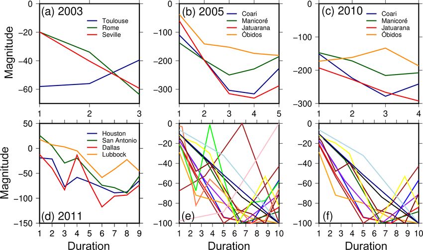
232                          H. Gerdener et al.: Gravity Recovery and Climate Experiment (GRACE) drought indicators

Figure 2. Concept of the synthetic framework to generate synthetic TWSC.

compute temporal signal correlations by fitting an autore-           a signal representative of the mean conditions within the re-
gressive (AR) model (Appendix A; Akaike, 1969) to de-                gion, and they are then used to create the constant, trends, and
trended and deseasoned GRACE data. These TWSC residu-                the seasonal parts of the synthetic time series. To simulate re-
als contain interannual and subseasonal signals including real       alistic temporal correlations at the regional scale (step 2), we
drought information. Next, temporal correlation coefficients         use the AR model identified beforehand (Fig. 2) and again
are used as an input for expectation maximization (EM) clus-         average AR model coefficients within the cluster. Then, we
tering (Dempster et al., 1977; Redner and Walker, 1984) be-          apply an AR model with the estimated optimal order and
cause regions with similar residual TWSC correlation within          the averaged correlation coefficient (Eq. A1) to the synthetic
the interannual and subseasonal signal are hypothesized here         time series to add temporal correlations.
to be more likely affected by the same hydrological pro-                Simulating realistic drought events in step 3 is challeng-
cesses. The EM algorithm by Chen (2018) is modified to               ing because, to our knowledge, no unique procedure to sim-
identify regional clusters. The EM algorithm alternates an           ulate realistic drought periods for TWSC exists. For this rea-
expectation and a maximization step to maximize the like-            son, we first perform a literature review to identify represen-
lihood of the data (e.g., Dempster et al., 1977; Redner and          tative drought periods and magnitudes for selected regions.
Walker, 1984; Alpaydin, 2009). More details about EM clus-           Among others, this includes the 2003 European drought and
tering are provided in Appendix B.                                   the drought in the Amazon basin in 2011 (e.g., Seitz et al.,
   As a result of this procedure, we identified three clusters       2008; Espinoza et al., 2011, respectively). TWSC data within
located in eastern Brazil (EB), southern Africa (SA), and            the identified drought period are then eliminated from the
western India (WI), which were indeed affected by droughts           time series. In the next step, the parameters describing the
in the past (e.g., Parthasarathy et al., 1987; Rouault and           constant, trend, acceleration, and seasonal signal compo-
Richard, 2003; Coelho et al., 2016). The location and shape          nents before and after the drought are used to “extrapolate”
of the three chosen clusters are shown in Fig. 3, and a global       these signals during the drought period. By computing the
map of all clusters is provided in Fig. B1. Cluster delin-           difference of the original GRACE-TWSC time series and
eations from the above procedure should not be confused              the continued signal in the drought period, we can separate
with political boundaries or watersheds. The following sim-          non-seasonal variations from the data, which represent the
ulation steps are then applied to each of these three clusters.      drought magnitude. Our hypothesis is that the non-seasonal
   In step 1 we estimate the signal coefficients according to        variations that we derive from the procedure possibly show a
Eq. (18) through least squares fit for each grid cell within the     systematic behavior that can be parameterized. To extract this
cluster. The coefficients are then spatially averaged to create      systematic behavior, all extracted droughts are transformed

Hydrol. Earth Syst. Sci., 24, 227–248, 2020                                         www.hydrol-earth-syst-sci.net/24/227/2020/
H. Gerdener et al.: Gravity Recovery and Climate Experiment (GRACE) drought indicators                                         233

Figure 3. AR(1) model coefficients (–) for global GRACE-TWSC. The polygons of the clusters of eastern Brazil, southern Africa, and
western India are added in magenta.

to a standard duration. To compare the different drought sig-      work enables us to identify strengths and weaknesses of each
nals, a standard duration and a standard magnitude are arbi-       analyzed indicator, and it thereby enables us to choose the
trarily set to 10 months and −100 mm, respectively. Finally,       most suitable indicator for a specific application.
a synthetic drought signal η is generated by using the ex-
tracted knowledge of drought duration, drought magnitude,          3.2   Synthetic TWSC
and systematic behavior, and it is added to the synthetically
generated signal (Eq. 20).                                         Here, we will briefly discuss the TWSC simulation following
   In step 4 we add GRACE-specific spatially correlated and        methods described in the previous section.
temporally varying noise  (Eq. 20). First, for each month t          When estimating AR models for detrended and desea-
we extract a full variance–covariance matrix 6 for the re-         soned global GRACE data, we find that for more than 70 %
gion grid cells from GRACE-TWSC. Then, whenever 6 is               of the global land TWSC grids are best represented by an
positive definite, we apply the Cholesky decomposition 6 =         AR(1) process (Fig. A1). Therefore, we apply the AR(1)
RT R, while if 6 is only positive semi-definite, we apply          model for each grid. Figure 3 shows the estimated AR model
eigenvalue decomposition (Appendix C). Second, we gen-             coefficients, which represent the temporal correlations, rang-
erate a Gaussian noise series v of the length n, where n rep-      ing from very low up to 0.3, e.g., over the Sahara or in south-
resents the number of grid cells within the cluster. Finally,      western Australia, up to about 0.8, e.g., in Brazil or in the
spatial noise in month t is simulated through                      southeastern US. EM clustering is then based on these coef-
                                                                   ficients.
 = RT v.                                                 (21)        The selected three clusters (Fig. 3) show differences be-
                                                                   tween the signal coefficients of the functional model (step 1;
The final synthetic signals for each grid cell within a cluster    Eq. 18), which are hence discussed for the linear trend. We
will thus exhibit the same constant, trend, acceleration, sea-     find a mean linear trend for the eastern Brazil cluster of
sonal signal, temporal correlations, and drought signal, but it    1.0 mm TWSC per year, a higher trend of 5.0 mm per year
has spatially different and correlated noise. In the following,    in southern Africa, and for western India a trend of 56.3 mm
we will test the hypothesis that GRACE indicators depend           per year (Table 3). The trends for eastern Brazil and south-
on the presence of trend and random input signals using the        ern Africa in GRACE-TWSC have been identified before
generated synthetic time series.                                   (e.g., Humphrey et al., 2016; Rodell et al., 2018). We did not
   We believe that our synthetic framework based on real           find confirmations for the strong linear trend in western India
GRACE data has multiple benefits: (i) we are able to identify      found, for example, by Humphrey et al. (2016), who identi-
the ability of an indicator by comparing the true drought du-      fied about 7 mm per year within this region. We assume that
ration and magnitude (step 3) to the indicator results; (ii) we    in this study the linear trend for western India is estimated as
are able to detect the influence of other typical GRACE sig-       strong positive because we additionally identify a strong neg-
nals on the drought detection; and (iii) the synthetic frame-      ative acceleration of −8.03 mm yr−2 in western India. How-

www.hydrol-earth-syst-sci.net/24/227/2020/                                         Hydrol. Earth Syst. Sci., 24, 227–248, 2020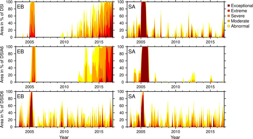
234                         H. Gerdener et al.: Gravity Recovery and Climate Experiment (GRACE) drought indicators

ever, our simulation will cover weak and strong trends. In        4     Indicator-based drought identification with synthetic
fact, all coefficients show strong differences, which suggests          and real GRACE data
that we cover different hydrological conditions when simu-
lating TWSC for the three regions. In step 2 we identify cor-     4.1    Synthetic TWSC: masking effect of trend and
relations of 0.74 in eastern Brazil, 0.79 in western India, and          seasonality
0.42 in southern Africa (Table 3).
   Performing literature research for drought duration and        Here, we analyze how non-drought signals, such as a lin-
magnitude (step 3) led to four droughts seen in GRACE-            ear or accelerated water storage trend and the ubiquitous
TWSC (Table 4): the 2005 and 2010 droughts in the Ama-            seasonal signal, propagate through the Zhao, Houborg, and
zon (e.g., Chen et al., 2009; Espinoza et al., 2011), the         Thomas GRACE indicators (Sect. 2) and potentially mask
2011 drought in Texas (e.g., Long et al., 2013), and the          a drought. To this end, we select representative time series
2003 drought in Europe (e.g., Seitz et al., 2008). To extract     from each of the three synthetic grids of total water storage
the drought duration, we compared drought onset and end           changes for eastern Brazil, southern Africa, and western In-
identified in these and other papers. We found that different     dia and apply the three methods. Since all results are based
studies do not exactly match, with inconsistencies likely due     on TWSC, we refer to TWSC-DSIA, TWSC-DSID, TWSC-
to different methodologies used. Furthermore, some authors        DIA, and TWSC-DID as DSIA, DSID, DIA, and DID, re-
only specified the year of drought. Droughts extracted from       spectively (again, with accumulated (A) and differenced (D)
the literature had a duration of 3 to 10 months (Fig. 4a–d).      variants).
Unless otherwise specified, we decided to base our simula-           We first assess the temporal characteristics of the Zhao
tions on a duration of 9 months to represent a clear identi-      method (Sect. 2.1). Figure 6 (left) shows time series for the
fiable drought duration. Extracted drought magnitudes range       DSI and DSIA (with 3, 6, 12, or 24 months of accumulated
from about −20 to −350 mm TWSC (Fig. 4a–d). Therefore,            TWSC). It is obvious that trend and acceleration propagate
in order to simulate a drought magnitude that has a clear in-     into both DSI and DSIA (see eastern Brazil and western
fluence on the synthetic time series, we set the magnitude to     India). Resulting indicator values (e.g., for the years 2015
−100 mm.                                                          and 2016) are lower than those compared to a small trend
   As described in Sect. 3.1, we transform these water stor-      (southern Africa) and this may lead to misinterpretations be-
age droughts to a standard duration and magnitude to un-          cause a severe-to-mild drought is identified (−2 to −0.5),
derstand whether a typical signature can be seen. However,        while none is actually simulated. In contrast, the actual simu-
Fig. 4e remains inconclusive as there are, in particular, four    lated drought in 2005 is only identified as a moderate drought
standardized droughts, which show a very different temporal       (values up to −1.0) for EB.
behavior: Toulouse in 2003, Óbidos in 2010, and Houston              In the presence of a small trend (5.0 mm yr−1 ) and accel-
and Dallas in 2011. When we remove those four time series         eration (−0.38 mm yr−2 ; Table 3, SA), we do identify an ex-
(Fig. 4f), a systematic behavior can be identified and parame-    ceptional drought (Fig. 6 DSIA for southern Africa). This
terized using a linear or quadratic temporal model. However,      shows that the drought strength that we chose does indeed
due to these difficulties, we decided to use the most simple      lead to a correct identification of exceptional drought if no
TWSC drought model, i.e., a constant water storage deficit        masking occurs (but in the presence of GRACE noise), so
within a given time span.                                         at this point we can determine that exceptional drought rep-
   In step 4, we project the simulation on a 0.5◦ grid and        resents the true drought severity class. As expected, a trend
add spatially correlated GRACE noise. A few representa-           and/or an acceleration signal that are frequently observed in
tive time series of the gridded synthetic total water stor-       GRACE analyses can lead to misinterpretations in the indica-
age change are shown in Fig. 5 for eastern Brazil, south-         tors. However, the influence of the trend or acceleration also
ern Africa, and western India for the GRACE time period           depends on the timing of the drought period within the anal-
from January 2003 to December 2016. The effect of realis-         ysis window. For example, assuming we simulate the time
tic GRACE noise (dark blue vs. light blue) is clearly visible,    series with the same trend or acceleration but the drought
particularly for the SA case with low annual amplitude. The       were to occur in 2014, the drought detection would not have
synthetic drought period is placed from January to Septem-        been influenced as much. Therefore, we decided to set up an
ber 2005 (light brown) in all three regions. Synthetic TWSC       additional experiment and discuss the influence of different
variability includes considerable (semi-)annual variations for    trend strengths for the drought detection (Sect. 4.3).
EB based on Table 3. Furthermore, a strong negative accel-           The analysis reveals that DSI and DSIA indicators are
eration is contained in the synthesized time series for eastern   sensitive with respect to trends, while they are less sensi-
Brazil (Table 3) leading to strong negative TWSC towards          tive to the annual and semi-annual signal. The seasonal sig-
the end of the time series. For western India a strong positive   nal is clearly dampened (e.g., compare Fig. 5 to the DSIA
trend leads to low TWSC at the begin of the time series.          in Fig. 6). This is caused by removing the climatology
                                                                  within the Zhao method (Eq. 8). Comparing DSIA3, DSIA6,
                                                                  DSIA12, and DSIA24, e.g., for eastern Brazil, suggests that

Hydrol. Earth Syst. Sci., 24, 227–248, 2020                                       www.hydrol-earth-syst-sci.net/24/227/2020/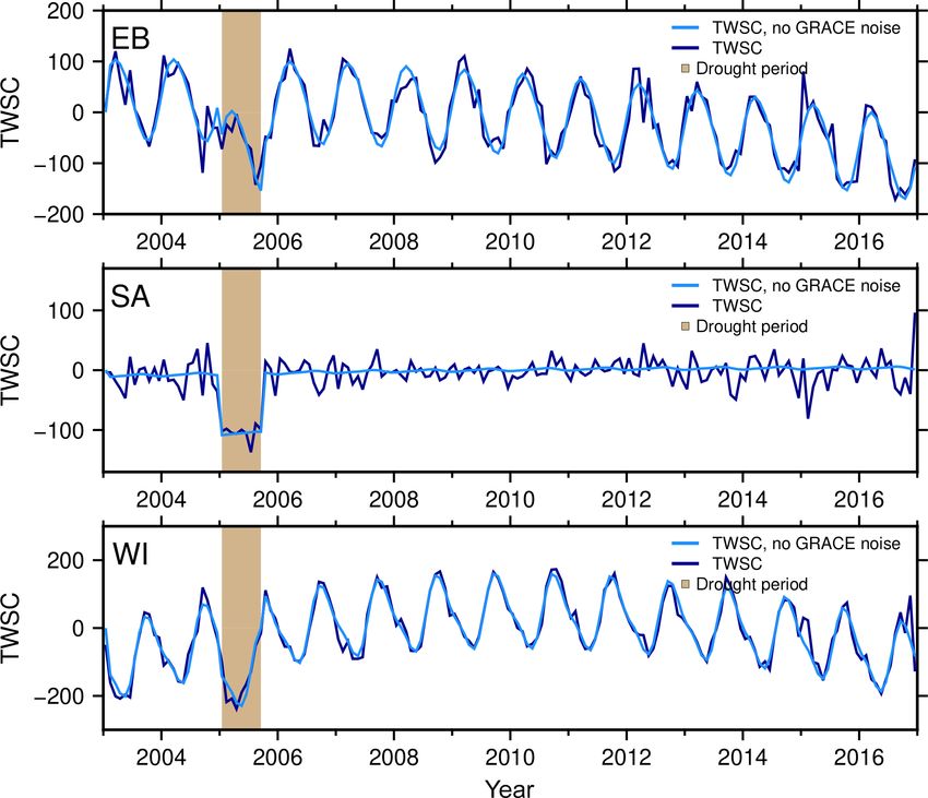
H. Gerdener et al.: Gravity Recovery and Climate Experiment (GRACE) drought indicators                                               235

Table 3. Coefficients (a0 to c2 from Eq. 18 and φ1 from Eq. A1) for signals contained in GRACE-TWSC that were extracted within the
clusters of eastern Brazil, southern Africa, and western India. These coefficients are used to simulate synthetic TWSC.

           Cluster           Constant    Linear    Acceleration         Annual                Semi-annual       AR-correlation
                                    a0     trend        a2             b1          b2            c2       c2          φ1
                                              a1
           Eastern Brazil      34.85       1.02       −1.77          6.83     106.12          4.69      9.47         0.74
           southern Africa    −24.00       4.98       −0.38         −4.31     −2.34          −1.23      1.07         0.42
           Western India     −139.37      56.30       −8.03         30.23    −122.69        −24.22     25.24         0.79

Figure 4. Extracted drought periods from GRACE-TWSC for the droughts in (a) Europe in 2003, (b) the Amazon river basin in 2005, (c) the
Amazon river basin in 2010, and (d) Texas in 2011. (e) All droughts from (a)–(d) were transformed to standard severity and duration. Panel
(f) is the same as (e) but after removing four time series with significant temporally different behavior.

with a longer accumulation period, indicator time series are           show a strong negative peak within the drought period, but
increasingly smoothed, and less severe droughts are identi-            this peak does not cover the entire drought period for the 3-,
fied (Fig. 6, left). Furthermore, the drought period appears           and 6-month differenced DSID. The negative peak within the
shifted in time, and its duration is prolonged. This can lead          drought period is always followed by a strong positive peak;
to missing a drought identification if a trend or an acceler-          when we consider Eq. (2), this lends to the interpretation
ation is contained in the analyzed time series, for example            that a pronounced drought period is normally followed by
for the 24-month DSIA for eastern Brazil. We find that all             a very wet event to return to “normal” water storage condi-
DSIA data are able to unambiguously detect a drought close             tion. Despite higher noise and the positive peak and contrary
to 2005, assuming that neither trend nor acceleration is ap-           to the DSIA, all DSID data (DSID3, DSID6, DSID12, and
parent (Fig. 6 DSIA for southern Africa). Particularly, the 3-         DSID24) correctly identify the drought within 2005 to be ex-
and 6-month DSIA data identify the drought close to 2005               ceptionally dry for eastern Brazil and southern Africa. All
for southern Africa, and its computation appears to dampen             different DSID time series for WI identify at least a moder-
the temporal noise that is present in the DSI.                         ate drought.
   In contrast we find that the 3-, 6-, 12-, and 24-month                 Analysis of the Houborg method shows a broadly simi-
TWSC-differencing DSID data exhibit stronger temporal                  lar behavior as compared to the Zhao method: the sensitiv-
noise as compared to the DSIA and the DSI. This can be                 ity of drought detection to an included trend or acceleration
seen in the light of Eq. (2) – these indicators are closer to me-      depends on the indicator type. Using the DIA we can con-
teorological indicators and thus do not inherit the integrating        firm the large influence of the trend or acceleration on the
property of TWSC. The DSID does not propagate a trend and              indicator value, which is not the case for DID (e.g., Fig. 7
acceleration, annual signal, or semi-annual signal. All DSID           DIA and DID for eastern Brazil). Annual and semi-annual
time series, for example for eastern Brazil (Fig. 6, right),           water storage signals are all considerably weakened in the

www.hydrol-earth-syst-sci.net/24/227/2020/                                              Hydrol. Earth Syst. Sci., 24, 227–248, 2020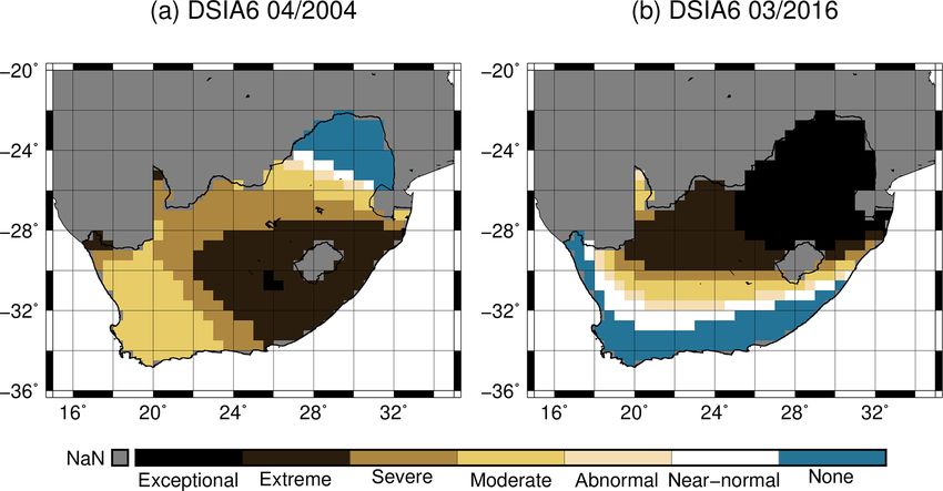
236                           H. Gerdener et al.: Gravity Recovery and Climate Experiment (GRACE) drought indicators

Table 4. Drought events in Europe, the Amazon river basin, and Texas with corresponding duration taken from the literature.

                          Region                Year of        Considered         Examples in the literature
                                                drought       TWSC months
                          Europe                  2003        June to August      Andersen et al. (2005)
                                                                                  Rebetez et al. (2006)
                                                                                  Seitz et al. (2008)
                          Amazon river basin      2005      May to September      Chen et al. (2009)
                                                                                  Frappart et al. (2012)
                                                  2010      June to September     Espinoza et al. (2011)
                                                                                  Frappart et al. (2013)
                                                                                  Humphrey et al. (2016)
                          Texas                   2011     February to October    Humphrey et al. (2016)
                                                                                  Long et al. (2013)

Figure 5. Synthetic TWSC (mm) without (light blue) and with spatial GRACE noise (dark blue) using average parameters for the clusters in
eastern Brazil (EB), southern Africa (SA), and western India (WI). Light brown shows the simulated drought period.

Houborg method because they are effectively removed when               have about 14 years of good monthly observations, so the
computing the empirical distribution for each month of the             simulation was also restricted to this period. If we then take
year. Differences to the Zhao method appear when compar-               the driest value that might occur only once, we can compute
ing more general properties; e.g., we find that DI is more             the minimum value of DI to be 7.14 %. Hence the detection
noisy and the range of output values is restricted to about 7 %        of a period of exceptional or extreme drought is not possible
to 100 % (Fig. 7). This restriction is caused by the length of         when referring to the duration of the GRACE-TWSC time se-
the time series; e.g., assuming we strive to identify an event         ries. As mentioned in Sect. 2.2, Houborg et al. (2012) applied
with exceptional dry values (≤ 2 %), we would need at least            a bias correction to the empirical CDF to mitigate this restric-
50 years of monthly observations. Yet, with GRACE we only              tion. We do not follow Houborg’s approach here in order to

Hydrol. Earth Syst. Sci., 24, 227–248, 2020                                            www.hydrol-earth-syst-sci.net/24/227/2020/
H. Gerdener et al.: Gravity Recovery and Climate Experiment (GRACE) drought indicators 237 Figure 6. A representative example of the synthetic DSI, DSIA, and DSID (–) for the eastern Brazil (EB), southern Africa (SA), and western India (WI) cluster over the periods of 3, 6, 12, and 24 months. Light brown shows the synthetic constructed drought period. Figure 7. A representative example of the synthetic DI, DIA, and DID (%) for the eastern Brazil (EB), southern Africa (SA), and western India (WI) cluster over the periods of 3, 6, 12, and 24 months. Light brown shows the synthetic constructed drought period. www.hydrol-earth-syst-sci.net/24/227/2020/ Hydrol. Earth Syst. Sci., 24, 227–248, 2020
238 H. Gerdener et al.: Gravity Recovery and Climate Experiment (GRACE) drought indicators
focus on the synthetic environment instead of the availability (exceptional) drought severity class. Yet we find that for both
of model outputs. DSI and DI the identification of drought severity is not sen-
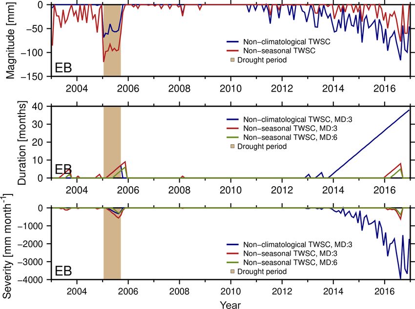
The Thomas method is applied to simulated TWSC data sitive to the choice of the averaging method for this clus-
to derive the magnitude, duration, and severity of a drought, ter. However, for other cases these differences can be more
which we show in Fig. 8 for the EB region. We find that the significant. These may lead to misinterpretation (e.g., May
linear trend and acceleration propagate into the magnitude and July 2005 for the DI for eastern Brazil, Fig. 9). For
(Fig. 8, top) when using TWSC deficits with climatology re- the Thomas method, we cannot distinguish which result is
moved (blue, Eq. 6) compared to using TWSC deficits with more significant, since we have no comparable true severity
removed trends, accelerations, and seasonality (red, Eq. 18). amount for that indicator.
When using non-climatological TWSC (blue), we identify a To determine the influence of the GRACE-specific spatial
strong deficit in 2015 and 2016 (Fig. 8, top), which suggests noise on the detected drought severity, a second analysis is
a duration of up to 38 months (Fig. 8, center) and a severity applied. This analysis computes the share of the area for each
of about −4000 mm months (Fig. 8, bottom). Using the de- time step for which a given drought severity class is identi-
trended and deseasoned TWSC (red), drought is mainly de- fied (Fig. 10). Since different grid cells for one time step only
tected in the true drought period (2005) and not at the end of differ in their spatial noise, it is important to understand that
the time series. Thus we conclude that a trend or acceleration identifying more than one severity class is directly related to
indeed modifies the drought detection. the noise. Only one class of drought would be detected for
Results so far were derived by imposing a minimum du- one epoch, assuming the grid cells have no or exactly the
ration of 3 months (blue and red). When moving to a mini- same noise. For example, we identify all classes of droughts
mum duration of 6 consecutive months (green, Fig. 8, middle (abnormal to exceptional) in December 2015 by using DSI
and bottom) we find this would lead to a decrease in identi- for the eastern Brazil cluster (Fig. 10, top left). Thus, the spa-
fied severity by half, and the beginning of the drought period tial noise has a large influence on the drought detection. To
shifts 3 months in time. This is in line with Thomas et al. establish which indicator is most affected, the indicators are
(2014). The same findings are made for southern Africa and compared with each other.
western India. We note that large differences are found between DSI, the
6-month accumulated DSIA, and the 6-month differenced
4.2 Synthetic TWSC: effect of spatially correlated DSID within the given drought period for the eastern Brazil
GRACE errors region (Fig. 10, left). All three indicators manage to identify
the drought, but they also do so with a different duration and
Here, we investigate how robust the Zhao, Houborg, and percentage of the affected area. Within the simulated drought
Thomas indicators are with respect to the spatially corre- period, the DSI indicator identified no more than 14 % of all
lated and time-variable GRACE errors. However, any anal- grid cells as being affected by exceptional drought where it
ysis must take into account that GRACE results cannot be should be 100 %. On the other hand, the DSIA does not de-
evaluated directly at grid resolution. tect exceptional drought in any grid cell. It is apparent that
In our first analysis, indicators based on (synthetic) TWSC this indicator misses the exceptional dry event because of the
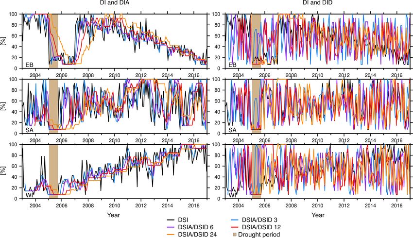
grids are thus spatially averaged through two different meth- included trend and acceleration.
ods (Sect. 3.1). We find that regional-scale DSI and DI indi- When comparing the DSIA of eastern Brazil to the DSIA
cators, as well as the outputs derived by the Thomas method of southern Africa (Fig. 10, center), we find that DSIA is able
for southern Africa computed from averaging TWSC first to detect the drought strength correctly when there is a small
(dark blue Fig. 9), are indeed different to the averaging in- trend or acceleration present. However, DSIA appears more
dicators computed at grid scale from TWSC (light blue, robust against spatial noise, since it identifies severe drought
Fig. 9). These differences can be explained by the inherent or drier in more than 90 % of grid cells, while the DSI indi-
non-linearity of the indicators. Since the synthetic data have cator identifies only about 60 %. As described in Sect. 4.1,
been constructed from the same constants, trends, seasonal longer accumulation periods lead to smoother and thus more
signal, temporal correlations, and drought signal, we isolate robust indicators. We find that the DSID is more success-
the effect of GRACE noise on regional-scale indicators here. ful in detecting exceptional drought: more than 80 % of the
Outside of the drought period we conclude that the sequence DSID grid cells show exceptional drought, but the indica-
in which we spatially average causes larger differences for DI tor appears more noisy than DSIA. Finally, with regard to
as compared to DSI. For southern Africa, the range of aver- the drought duration, we find that only DSI detects the true
aged DI is about 7 %–100 %, while the range of the DI of period correctly. When identified via DSIA, the duration ap-
averaged TWSC is about 7 %–80 %. Within the drought pe- pears longer, and when identified in DSID, the period was
riod the DI exhibits little difference between both averag- found shorter as compared to the true drought period.
ing methods. The DSI from averaged TWSC does suggest a Overall, we find that the different indicators of DSI, DSIA,
weaker severity in the drought period compared to averaged and DSID all come with advantages and disadvantages re-
DSI. In this case, both indicator averages identify the same garding the presence of spatial and temporal noise. The
Hydrol. Earth Syst. Sci., 24, 227–248, 2020 www.hydrol-earth-syst-sci.net/24/227/2020/H. Gerdener et al.: Gravity Recovery and Climate Experiment (GRACE) drought indicators 239
Figure 8. Drought magnitude (mm), duration (months) and severity (mm month−1 ) for the cluster in eastern Brazil (EB) using TWSC
with the removed climatology (dark blue) and TWSC with removed trend and seasonal signal (red). The minimum duration (MD) is set to
3 months (blue and red) or 6 months (green). Light brown shows the synthetic constructed drought period.
same findings were made for the indicators of the Houborg trend, i.e., whether the trend is positive or negative. Assum-
method (results not shown). This analysis is not applied to ing that a positive trend exists and the drought occurs closer
the Thomas method, because the method does not refer to to the end of the time series, the trend may lead to a drought
severity classes (Sect. 2.3). that is identified as more dry than the true drought. But if the
trend is negative, the drought is identified more easily.
4.3 Synthetic TWSC: experiments with variable trend, Other factors, e.g., the length of the time series, have an
drought duration, and severity influence on the masking by the trend and, as a result, af-
fect drought detection. The longer the input time series, the
Two experiments were additionally constructed to examine more sensitive the drought detection is to the trend. At the
the influence of trends and drought parameters on the indica- same time, the magnitude of the trend needs to be considered
tor capability. First, we consider how strong a linear trend in relative to the variability or range of TWSC. For example, a
total water storage must be to mask drought in the indicators. −6 mm yr−1 trend has a larger influence on the drought de-
For this, we test different trends from −10 to 10 mm yr−1 for tection if the range of TWSC is −50 to 50 mm compared to
DSI, DSIA, DI, DIA, and the Thomas method in the western −200 to 200 mm. As a reference, the synthetic time series
India region (since these indicators were identified as being for western India, without any trend or acceleration signal,
affected by trends; Sect. 4.1). No acceleration is included for ranges from about −323 to 87 mm. So, deriving a general
these tests. We find that trends between −1 and 1 mm yr−1 quantity for these dependencies is difficult.
cause no influence on all indicators, while differences start In a second experiment, we assess which input drought
to appear when simulating a trend higher than 2 mm yr−1 . duration and magnitude would at least be visually recog-
This propagates into the DSI, DSIA, DI, and DIA indicators nized in the indicators. We choose 3, 6, 9, 12, and 24 months
but did not affect the drought period. for the simulated duration and −40, −60, −80, −100, and
A question we must ask is what would be the largest −120 mm for the drought magnitude and apply both the
trend magnitude that does not affect the correct detection of Zhao and the Houborg methods. We compare the changes for
drought duration and drought severity, and how can we verify one indicator time series for the eastern Brazil region. The
this. An obvious influence within the drought period in 2005 drought always begins in January 2005 for the first tests. In
is found when simulating a trend of −7 mm or lower per year. general, we found that the identification of the severity class
It is important at this point to understand that there is a rela- is less sensitive to changes in the drought duration, since a
tion between the timing of the drought and the sign of the drought duration of 3, 6, 9, 12, and 24 months mostly re-
www.hydrol-earth-syst-sci.net/24/227/2020/ Hydrol. Earth Syst. Sci., 24, 227–248, 2020240 H. Gerdener et al.: Gravity Recovery and Climate Experiment (GRACE) drought indicators Figure 9. DSI and DI average in southern Africa (SA; a, b), severity average for the Thomas method (SA; c), and DI average in eastern Brazil (EB, d) by applying two different methods: the average of the indicators for all grids (light blue) and the indicators of averaged TWSC (dark blue). The grey shaded area represents the bandwidth for all grids. Light brown shows the synthetic constructed drought period. sults in equal drought severity classes, for example, a drought both methods are not able to clearly detect a drought that has magnitude of 120 mm. Thus, we concentrate our analysis on a magnitude of −40 mm or weaker if the duration is between changes in drought magnitude. 3 and 24 months. This experiment supports our findings in Exceptional drought is only classified by the Zhao method Sect. 3.2. for eastern Brazil for a simulated drought magnitude of 120 mm; this is related to the trend and acceleration signal 4.4 Application to real GRACE data: droughts in contained in the simulated TWSC and was already found in South Africa Sect. 4.1. For the Zhao method, extreme drought is identified when simulating a drought magnitude of at least −100 mm, For South Africa, droughts are a recurrent climatic phe- while only a period of severe and moderate drought is identi- nomenon. The complex rainfall regime has led to multiple fied when simulating a magnitude of −80 and −60 mm. The occurrences of drought events in the past, for example to a Houborg method fails to identify extreme and exceptional strong drought in 1983 (e.g., Rouault and Richard, 2003; Vo- drought, as described in Sect. 4.1. Thus, simulating a mag- gel et al., 2010; Malherbe et al., 2016). These past droughts nitude of −100 and −120 mm is identified as severe drought appeared in varying climate regions, at different times of the for all simulated drought periods (3 to 24 months), while sim- year, and with a different severity. Since 1960, many of them ulating a lower magnitude (−80 and −60 mm) causes mod- were linked to El Niño (e.g., Rouault and Richard, 2003; erate or abnormal dry events to be identified. We find that Malherbe et al., 2016). Hydrol. Earth Syst. Sci., 24, 227–248, 2020 www.hydrol-earth-syst-sci.net/24/227/2020/
H. Gerdener et al.: Gravity Recovery and Climate Experiment (GRACE) drought indicators                                               241

Figure 10. Drought-affected area of the DSI, DSIA, and DSID (%) considering the different drought severity classes within the clusters of
eastern Brazil (EB) and southern Africa (SA).

Figure 11. Percentage of drought-affected area for the 6-month DSIA (–) considering the different drought severity classes. Application on
real GRACE-TWSC over South Africa from 2003 to 2016.

   Based on the simulation results, we chose the 6-month ac-           drought in 2004 mainly occurred in central and southeastern
cumulated DSIA to identify droughts for (the administrative            South Africa; this is exemplified in Fig. 12a for April 2004.
area of) South Africa (GADM, 2018) in the GRACE total                  Another confirmation is found in Malherbe et al. (2016),
water storage data. DSIA has proven to be more robust with             who identified a drought period from 2003 to 2007 by using
respect to the peculiar, GRACE-typical spatial and temporal            the SPI.
noise as compared to the other tested indicators (Sect. 4.1               Despite affecting less area (about 50 % to 70 %; Fig. 11),
and 4.2).                                                              the second drought in 2015 and 2016 is perceived as more
   GRACE-DSIA6 suggests two drought periods, from mid-                 intense than the drought from 2003 to 2006. Based on the
2003 to mid-2006 and from 2015 to 2016 (Fig. 11). The first            GRACE-DSIA6 data, we conclude that in 2016 at least 30 %
drought event is identified to affect at least 70 % of the area of     of South Africa was affected by extreme drought and about
South Africa. While 2003 was indeed a year of abnormal-to-             20 % experienced an exceptional drought. The 2016 drought
severe dry conditions, extreme drought occurred during the             occurred in the northeastern part of South Africa (Fig. 12b).
period of 2004 to mid-2006. Figure 11 reveals that a small             For comparison, the EM-DAT database similarly identi-
area (about 7976 km2 , close to Lesotho) even experienced ex-          fied 2015 as a drought event, but it did not classify 2016 as
ceptional drought during 2004. This period is confirmed by             such. We speculate that the differences are due to the drought
the Emergency Events Database (EM-DAT, 2018) recording                 criteria of EM-DAT (disasters are included when, for exam-
of a drought event in 2004 (e.g., Masih et al., 2014). Extreme         ple, 10 or more people died or 100 or more people were af-

www.hydrol-earth-syst-sci.net/24/227/2020/                                              Hydrol. Earth Syst. Sci., 24, 227–248, 2020
You can also read