African soil properties and nutrients mapped at 30 m spatial resolution using two scale ensemble machine learning
←
→
Page content transcription
If your browser does not render page correctly, please read the page content below
www.nature.com/scientificreports
OPEN African soil properties
and nutrients mapped at 30 m
spatial resolution using two‑scale
ensemble machine learning
Tomislav Hengl1,2*, Matthew A. E. Miller3, Josip Križan4, Keith D. Shepherd5,
Andrew Sila5, Milan Kilibarda6, Ognjen Antonijević6, Luka Glušica7, Achim Dobermann8,
Stephan M. Haefele9, Steve P. McGrath9, Gifty E. Acquah9, Jamie Collinson3,
Leandro Parente2, Mohammadreza Sheykhmousa2, Kazuki Saito10, Jean‑Martial Johnson10,
Jordan Chamberlin11, Francis B. T. Silatsa12, Martin Yemefack12, John Wendt13,
Robert A. MacMillan2, Ichsani Wheeler1,2 & Jonathan Crouch3
Soil property and class maps for the continent of Africa were so far only available at very generalised
scales, with many countries not mapped at all. Thanks to an increasing quantity and availability of
soil samples collected at field point locations by various government and/or NGO funded projects,
it is now possible to produce detailed pan-African maps of soil nutrients, including micro-nutrients
at fine spatial resolutions. In this paper we describe production of a 30 m resolution Soil Information
System of the African continent using, to date, the most comprehensive compilation of soil samples
(N ≈ 150, 000) and Earth Observation data. We produced predictions for soil pH, organic carbon
(C) and total nitrogen (N), total carbon, effective Cation Exchange Capacity (eCEC), extractable—
phosphorus (P), potassium (K), calcium (Ca), magnesium (Mg), sulfur (S), sodium (Na), iron (Fe), zinc
(Zn)—silt, clay and sand, stone content, bulk density and depth to bedrock, at three depths (0, 20
and 50 cm) and using 2-scale 3D Ensemble Machine Learning framework implemented in the mlr
(Machine Learning in R) package. As covariate layers we used 250 m resolution (MODIS, PROBA-V
and SM2RAIN products), and 30 m resolution (Sentinel-2, Landsat and DTM derivatives) images.
Our fivefold spatial Cross-Validation results showed varying accuracy levels ranging from the best
performing soil pH (CCC = 0.900) to more poorly predictable extractable phosphorus (CCC = 0.654)
and sulphur (CCC = 0.708) and depth to bedrock. Sentinel-2 bands SWIR (B11, B12), NIR (B09, B8A),
Landsat SWIR bands, and vertical depth derived from 30 m resolution DTM, were the overall most
important 30 m resolution covariates. Climatic data images—SM2RAIN, bioclimatic variables and
MODIS Land Surface Temperature—however, remained as the overall most important variables for
predicting soil chemical variables at continental scale. This publicly available 30-m Soil Information
System of Africa aims at supporting numerous applications, including soil and fertilizer policies and
investments, agronomic advice to close yield gaps, environmental programs, or targeting of nutrition
interventions.
Predictive Soil Mapping (PSM) aims to produce the most accurate and most objective predictions of soil vari-
ables either for bulk estimates or for specific soil depths. PSM, a sub-field of Applied Predictive M
odeling1, can
be considered to be an interdisciplinary field incorporating statistics, soil science and Machine Learning2–5.
1
EnvirometriX Ltd, Wageningen, The Netherlands. 2OpenGeoHub Foundation, Wageningen, The
Netherlands. 3Innovative Solutions for Decision Agriculture Ltd (iSDA), Harpenden, United Kingdom. 4MultiOne
Ltd, Zagreb, Croatia. 5World Agroforestry (ICRAF), Nairobi, Kenya. 6Department of Geodesy and Geoinformatics,
Faculty of Civil Engineering, University of Belgrade, Belgrade, Serbia. 7GILAB Ltd, Belgrade, Serbia. 8International
Fertilizer Association (IFA), Paris, France. 9Rothamsted Research, Harpenden, United Kingdom. 10Africa Rice
Center (AfricaRice), Bouaké, Côte d’Ivoire. 11International Maize and Wheat Improvement Centre (CIMMYT),
Nairobi, Kenya. 12Sustainable Tropical Solutions (STS) Sarl, Yaoundéc, Cameroon. 13International Fertilizer
Development Center (IFDC), Muscle Shoals, AL, USA. *email: tom.hengl@envirometrix.net
Scientific Reports | (2021) 11:6130 | https://doi.org/10.1038/s41598-021-85639-y 1
Vol.:(0123456789)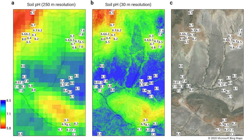
www.nature.com/scientificreports/
Training points used to build predictive models are usually provided by data from soil samples (fixed depth
intervals) or soil profiles (pedogenetic soil horizons) that were geolocated in the field and then entered into a
soil profile database. Covariate layers commonly used to train models include terrain a ttributes4—especially
hydrological terrain parameters—parent material maps, climatic and vegetation maps and surface reflectances,
including bare soil surface r eflectances6. Predictions of soil properties and classes are generated by (1) training
the learners i.e. fitting the spatial prediction models, then (2) applying these fitted models to all pixels so that a
complete and consistent map can be produced1,5.
Until recently, soil property and class maps for the continent of Africa were only available at very general-
ised scales7–9, with many countries not mapped at all. Considerable soil resources of Africa, especially organic
matter10 and nutrient s tocks11 remained largely unmapped and unknown. Fertilizer prices in Africa remain
discouragingly high and consequently the efficiency of using fertilizers needs to be clear and considerable before
it can be adopted by cash-constrained and risk averse farmers7,9,12. It is now possible to produce detailed maps
of soil nutrients, including micro-nutrients, due to increasing quantity and availability of soil samples collected
at field point locations by various government and/or NGO funded projects: e.g. by projects supported by the
National Governments of Ethiopia, Tanzania, Kenya, Uganda, Nigeria, Ghana, Rwanda, Burundi and others; by
international donors13–16, as well as by the private sector.
The AfSIS project released, in 2017, a gridded Soil Information System of Africa at 250 m resolution showing
the spatial distribution of primary soil properties of relatively stable nature, such as depth to bedrock, soil particle
size fractions (texture), pH, contents of coarse fragments, organic carbon and extractable elements such as Fe,
Ca, Mg, Na, K, Zn, Cu, Mn and A l17. The 250 m resolution predictions were later used to estimate large-scale
nutrient gaps i.e. fertility zones for major agricultural crops. Berkhout et al.18, for example, reported significant
relations between these soil nutrient maps and human health as indicated by child mortality, stunting, wasting
and underweight.
The initial maps produced in 2 01717 exhibited several limitations:
• Harmonization of training points (merge from multiple datasets) revealed problems with incomplete meta-
data which made the data less reliable. Predictions of extractable phosphorous (see Fig. 5 in Hengl et al.17),
for example, were shown to over-estimate values at multiple locations. Such systematic oscillations usually
arise due to incorrect use of measurements units or errors in importing the soil sample data.
• During this earlier predictive soil mapping exercise, spatial clustering of points (i.e. over-representation of
specific soil types and landscape positions) were not yet accounted for in the m ethodology19. This possibly
introduced a bias in the earlier 250 m scale predictions.
• Predictions were based on the use of relatively coarse resolution covariates only, with limited up-to-date
Earth Observation imagery available at that time to help map nutrient content.
We recently re-examined these problems and concluded that a complete redesign and re-implementation of
the entire PSM process was required, beginning from point data import and harmonization, into modeling and
spatial cross-validation methodologies. Our main hypothesis was that the accuracy of the previous predictions
could be much improved if we:
1. Utilize an improved predictive mapping framework: spatially-adjusted Ensemble Machine Learning, that
better accounts for spatial clustering of points;
2. Invest more effort into fine-tuning the Machine Learning algorithms: especially to account for spatial cluster-
ing of points, and more efficiently subset features of interest;
3. Include in the prediction process new, state-of-the-art, Earth Observation data: especially Sentinel-2 imagery
which is available for the entire continent at fine spatial resolutions (10–30 m);
4. Include per pixel error predictions i.e. to quantify prediction uncertainty per pixel.
In addition to redoing the spatial analysis of soil nutrients, we also decided to extend the original list of tar-
utrients17 to include soil chemical (pH, eCEC) and physical (bulk density, clay, sand and silt fractions)
get soil n
properties, so that we can produce a more holistic representation of soils.
We present here results of modeling and predicting soil variables for the entire African continent. These are
now made available at relatively detailed spatial resolution (30 m), with prediction uncertainty estimates included
per pixel. We focus here on the main results and discoveries that could potentially impact any similar continental
or global scale soil mapping projects, and then provide detailed explanation of steps followed.
Results
Goodness of fit and variable importance. The preliminary import of all soil data in Google Earth
Engine and subsequent correlation analysis with Sentinel-2 percentiles (for the period 2016–2019), Landsat-8
percentiles (for the period 2013–2019) revealed that there was indeed potential, especially for Sentinel-2 prod-
ucts, to use Earth Observation (EO) data to increase the accuracy of mapping of soil properties and nutrients
in Africa. These results clearly indicate predictive potential with the most correlated soil/environmental param-
eters being soil pH (Sentinel-2 B04, B12, B9), soil organic carbon (Sentinel-2 B04, B05, B11, B12) and clay
content determined by laser diffraction method (Sentinel-2 B11, B12, B8A) with respective best R-square based
on spatial tenfold cross-validation at 0.38, 0.32 and 0.26 (Fig. 1). For Mehlich3 extractable nutrients and micro-
nutrients, Sentinel-2 and Landsat-8 products commonly explained < 25% of observed variation, but were still
significant. In the case of Sentinel-1 products (HH, HV, HH/HV), detectable correlation with soil nutrients,
Scientific Reports | (2021) 11:6130 | https://doi.org/10.1038/s41598-021-85639-y 2
Vol:.(1234567890)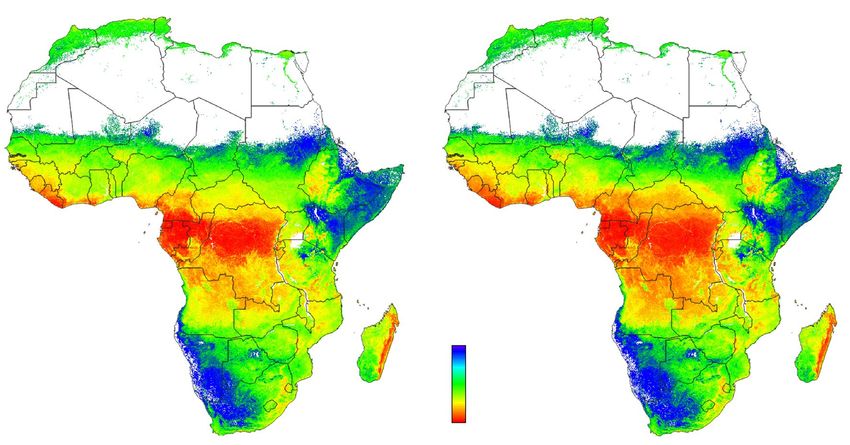
www.nature.com/scientificreports/
Figure 1. Preliminary predictive modeling R-square based on tenfold cross-validation and modeling selection
of soil target variables purely as a function of Sentinel-2 (a) and Sentinel-1 (b) products. Derived by uploading
soil data as points to Google Earth Engine, then overlaying with Sentinel-1/2 and Landsat products and fitting
individual models using the caret package1 (see also Fig. 7).
apart from pH and soil organic carbon, was considerably lower to non-existent (Fig. 1). For practical reasons,
we ultimately decided to focus on using existing Landsat p roducts20 and the Sentinel-2 bands B02 (Blue), B04
(Red), B8A (Narrow NIR), B09 (Water vapour), B11 (SWIR1) and B12 (SWIR2) as the major new environmental
covariates, while the Sentinel-1 products were not utilized to produce final predictions.
The combined variable importance plots derived using Random Forest with all 250 m and 30 m covariates
used together (Fig. 2) reveal that, on average, climatic images such as SM2RAIN monthly rainfall estimates and
CHELSA bioclimatic images (3, 7, 4), are the most important covariates to inform mapping of soil properties
and nutrients in Africa. This result is consistent with our previous global results21, where soil chemical proper-
ties were primarily correlated with climate images, and soil physical properties with a combination of landform
parameters, parent material and climatic images. At 30 m resolution, however, Sentinel-2 B11, B09 and B12, DTM
vertical depth and Landsat SWIR1 are overall the most important for mapping soil properties and nutrients.
Although these covariates appear lower on the full list of the most important variables than climatic images, this
is an important discovery and clearly indicates that Sentinel and Landsat seasonal and/or long-term composites
merit utilization as covariates for this current, and future, predictive soil mapping campaigns.
When the importance measures for all variables are ordered based on the mean relative importance (absolute
variable importance divided by the highest variable importance), the results show that overall the most important
variables for mapping soil properties in Africa are (1) sampling depth (Figs. 2 and 3), (2) Isothermality (quantifies
how large the day-to-night temperatures oscillate relative to the summer-to-winter annual oscillations) and (3)
mean annual rainfall. Here Isothermality seems to be especially important for modeling log ext.-K, log ext.-Mg
and log ext.-S, and mean annual rainfall for modeling organic carbon, organic N, soil pH, log ext.-Mg and log
ext.-P (see also Supplementary material).
The newly added USGS surficial lithology map of Africa22 did not help improve predictions, however ln-eCEC
values were significantly correlated with the class “Volcanic—Ash, Tuff, Mudflow”. Classes “Extrusive Volcanic”
and “Aeolian Sediments” seem to marginally help improve predictions of sand and clay. The surprisingly low
correlation between the surficial geology map classes and soil nutrients is most likely due to the overly coarse
scale of the geological map.
Accuracy assessment based on fivefold spatial cross‑validation. Table 1 shows summary results
of fivefold spatial cross-validation for all variables of interest. The average R-square ranges from the best per-
forming soil pH (CCC = 0.90) and ext.-Al (CCC = 0.937), to the worst performing ext.-P (CCC = 0.654), ext.-S
(CCC = 0.708) and depth to bedrock (CCC = 0.725). Also note from Table 1 that some variables are predicted
using considerably smaller training pools: especially bulk density, depth to bedrock, ext.-S and ext.-Zn have
about 2–3× fewer observations for training than e.g. soil pH or similar. The models for bulk density, depth to
bedrock, ext.-S and ext.-Zn are hence, in general, less representative of all landscape combinations in Africa and
should be used with caution.
The spatial Cross-Validation accuracy assessment results (Fig. 4) show that a combination of feature selection
and 2-scale modeling results in substantial improvements in prediction performance when compared to the
previous work17. Improvements in accuracy are especially substantial for ext.-K, ext.-Fe, ext.-P and ext.-Ca, i.e.
all variables where 30 m covariates can explain up to 30% of additional variation in the target variables.
The results of stacking various learners indicate that overall Random F orest23 seems to perform best in the
fivefold Cross Validation, followed by the Lasso and Elastic-Net Regularized Generalized Linear Models (regr.
cvglmnet)24, while Xgboost25 and deepnet26 packages only marginally increase accuracy of predictions.
Scientific Reports | (2021) 11:6130 | https://doi.org/10.1038/s41598-021-85639-y 3
Vol.:(0123456789)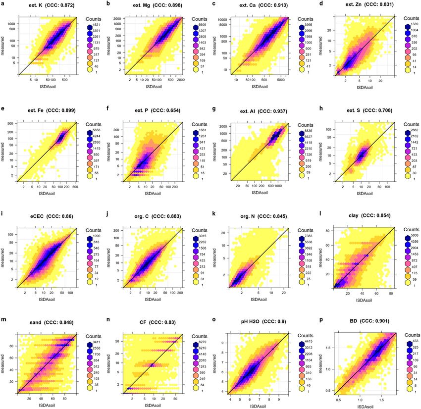
www.nature.com/scientificreports/
Figure 2. Relative covariate importance for selected target soil variables ordered based on mean importance
of all 250 m and 30 m resolution covariates. In this instance, the covariate “sampling depth” is the overall
most important covariate, while Sentinel-2 B11 and Landsat SWIR images are revealed as the highest ranked
covariates at 30 m resolution (see further Table 1 and Supplementary materials).
The model performance and individual variable importance lists can be also tracked via the https://zenodo.org
repositories for iSDAsoil.
In summary, in comparison to our previous work17, these accuracy results suggest an average improvement
in the R-square value from 0.6 (250 m predictions) to 0.8 (30 m predictions), probably primarily attributable to
the addition of higher resolution remote sensing images and Digital Terrain parameters, but also by the adoption
of methodological improvements in hyper-parameter tuning, feature selection and ensembling of models using
the Super Learner algorithm. Note also that, thanks to the AfSIS project, most of the points used for training
have been geo-located with high accuracy (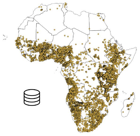
www.nature.com/scientificreports/
Figure 3. Example of predictions of soil pH 1:1 water suspension at 0 cm (a) and 50 cm (b) depths whole of
Africa. See also Fig. 2. Visualizations produced using QGIS v3.10 (https://www.qgis.org/).
Variable Unit Training samples R-square RMSE CCC
Sand content % 122,261 0.736 13.7 0.848
Silt content % 122,223 0.640 8.92 0.780
Clay content % 122,269 0.746 9.6 0.854
Bulk density,www.nature.com/scientificreports/
Figure 4. Accuracy assessment plots for all soil nutrients (a–h) and physical and chemical soil properties (i–p)
based on the final models used for prediction. Accuracy plots derived using fivefold spatial cross-validation.
Extractable nutrient concentrations expressed in mg/kg and displayed on a log-scale. CF Coarse fragments or
stone content, BD bulk density.
be verified if similar relations between soil organic carbon and 250 m resolution and 30 m resolution EO data
is also applicable on other continents.
Discussion
Over the last decade, the AfSIS project invested considerably in producing a new generation of agronomy data
for Africa via AfSIS and related projects. To further extend and derive additional benefit from this primary soil
data, we created an agronomy database at a previously unprecedented spatial resolution of 30 m, covering the
entire African continent. The newly produced data volumes are substantial: for illustration, one image of Africa
at 30 m resolution contains over 24 billion pixels of data (if shifting sand areas such as Sahara are excluded); the
average size of a Cloud-Optimized GeoTIFF with internal compression containing predicted values of proper-
ties was of the order of 10–20 GiB. By harnessing available Open Access remote sensing data (Sentinel 2, Land-
sat 7/8), 3D predictive machine learning techniques (ensemble between Random Forest, XGBoost, deepnet,
Cubist and GLM-net), and point samples generated by the AfSIS network, as well as a number of other open
access soil datasets, we have modeled and produced predictions of 18+ soil variables including: soil texture
fractions, soil pH, macronutrients (soil organic carbon, nitrogen, phosphorous, and potassium, magnesium),
Scientific Reports | (2021) 11:6130 | https://doi.org/10.1038/s41598-021-85639-y 6
Vol:.(1234567890)www.nature.com/scientificreports/
Figure 5. Illustration of differences in spatial detail of predictions for soil pH for top-soil: (a) previous
predictions at 250 m published in Hengl et al.17, (b) current predictions at 30 m, which seem to match very well
physical patterns seen on the satellite imagery (c). Sentinel site area in southern Kenya. Visualizations produced
using QGIS v3.10 (https://www.qgis.org/). Satellite image in c copyright 2020 Microsoft Bing Maps.
micronutrients, eCEC and others. The results indicate that the accuracy and spatial detail of previous maps can
be considerably improved with average R-square (based on spatial Cross Validation) improving from about 0.6
to values around 0.8.
Our experience is that the Ensemble Multi-scale Predictive Soil Mapping system is a robust, scalable system
which basically can be fully automated: from feature selection, model calibration and prediction, to determining
quantiles or standard deviation of the prediction error. This is mainly thanks to the flexibility of programming
in the mlr package28. The results of comparing different learners through fitting of meta-learners indicate that
Random Forest23 is the overall best-performing learner, but also Lasso and Elastic-Net Regularized Generalized
Linear Models and Cubist often perform equally well. Ensembling of multiple learners can be justified for most
of the target soil variables.
Mapping soil properties at 30 m and three depths with uncertainties is heavily computational and requires
substantial resources. Specifically, derivation of prediction errors can increase production costs considerably,
consequently these might need to be estimated using simplified procedures in the future. Also our main rationale
for using multiscale models vs one individual model was to try to decrease production costs without experienc-
ing a significant loss of accuracy. The results indicate that the 2-scale EML is especially attractive for reducing
computing costs which otherwise would have been about 5–10 times greater if we had tried to downscale ALL
of the covariates from 250 to the finest 30 m resolution.
We did not estimate the area of applicability for Machine Learning for Africa per soil variable following the
method of Meyer and Pebesma29, but our uncertainty maps do clearly reveal areas where the models extrapolate
or perform poorly: usually these are densely vegetated tropical areas (Congo basin) or semi-arid parts of Somalia
and Sudan. Next-generation soil sampling projects in Africa such as https://www.soils4africa-h2020.eu/ might
benefit from using our prediction uncertainty maps to identify new sampling locations e.g. by focusing on the
areas that are most difficult to model i.e. that have widest prediction error intervals.
In principle, 2-scale ensembling can be considered to provide a generic framework for predictive soil mapping.
It can be extended to consider multiple scales although, for practical purposes, we currently recommend using
a minimum of two and a maximum of three scales to avoid increasing the computational complexity unneces-
sarily. In practice, one could also begin by evaluating multiple scales, then select statistically significant scales,
then do ensembling of predictions for only scales identified as significant.
Value of the maps produced for local and/or field based agronomy needs to be evaluated “on the ground”
and by landowners/farmers. In the first few weeks of testing iSDAsoil app (see Fig. 6), we have already received
considerable feedback from experts in Europe and Africa. The main criticisms so far have focused on the low
accuracy of the SOC predictions, particularly for peatland areas, on sampling locations over-representing crop-
lands, and on problems with downloading and using these large datasets. The diversity of African soils and the
under-representation of specific areas remains a challenge.
Scientific Reports | (2021) 11:6130 | https://doi.org/10.1038/s41598-021-85639-y 7
Vol.:(0123456789)www.nature.com/scientificreports/
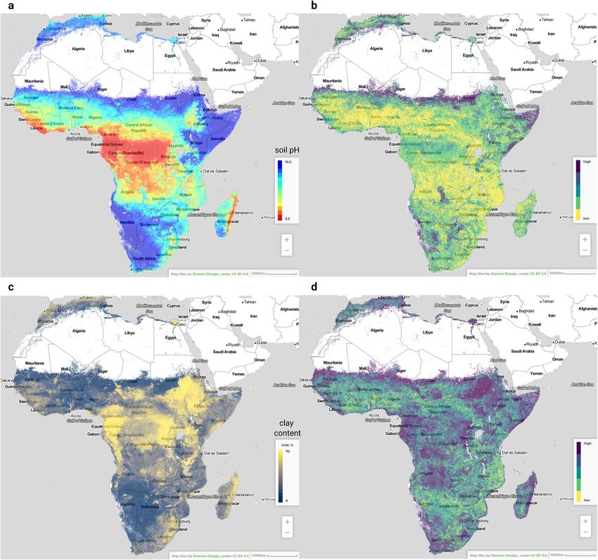
Figure 6. Predictions (left) and prediction uncertainty expressed as 1 s.d. prediction error (right), for soil pH
(a,b) and clay content (c,d) for the 0–20 cm depth interval. Visualized in the iSDAsoil app: https://isda-afric
a.com/isdasoil. The prediction error maps for clay content indicate that many areas probably require much more
samples than soil pH.
We note especially that the following aspects can be considered as requiring more and better training/point
data:
• Peatlands in Rwanda, Congo basin and similar remain heavily under-represented, as are all inaccessible
tropical jungles or similar remote areas.
• Nutrients P and S and micronutrients Cu, B remain difficult to map using current EO data and or any other
type of data available for use in this study. There seems to be no simple solution for this problem and possibly
not even 2× more point data for model training than we had here could guarantee success.
• Application (fertilizers), crop history, and similar data from field trials is generally lacking and available only
for limited locations e.g. via the Optimizing Fertilizer Recommendations for Africa (OFRA) d atabase30.
While there have been criticisms of the absolute accuracy of the iSDAsoil maps, it is important to consider this
in the context of real-world applications of the resource, for example in the generation of site-specific fertiliser
recommendations. In this case, additional data collection would be required such as land use history, previous
fertiliser applications and historic yields. However, we see this resource as a low cost alternative to lab-based soil
Scientific Reports | (2021) 11:6130 | https://doi.org/10.1038/s41598-021-85639-y 8
Vol:.(1234567890)www.nature.com/scientificreports/
test that has value in reducing uncertainty around soil properties compared to having no information, which is
especially relevant in a smallholder agriculture c ontext31.
Our initial predictions are not likely to be correct enough to support informed management at the farm
scale immediately. We can, however, propose our initial predictions as being relevant as a starting point, or base,
that drives and informs additional new sampling, for each specific parcel of interest. In that sense, our maps
provide a uniform and relevant base from which to start building individually relevant predictions for specific
parcels of agricultural land. Promotion of first steps for basic improved crop management does not perhaps
demand an exceptionally high accuracy of soil data. For example, a good estimate of soil pH can already help
to inform which crops may be most suitable to grow/ to not grow or if liming may be needed before any other
agrochemicals are used.
Collecting and adding point data from countries such as Democratic Republic of the Congo, Sudan and/or
Somalia remains a challenge as there are many serious security challenges for any soil sampling effort. Some
recent reports from the Congo have shown that tropical peatlands are probably heavily under-estimated in previ-
ous soil maps of Africa10,32. Even in relatively safe Tanzania, multiple human casualties occurred during the AfSIS
field data collection program, due to unclear land access permission and local militia problems. We anticipate,
nevertheless, that a large amount of publicly funded point samples and observations remain unavailable and
therefore unused33. These could be easily added to modeling and help improve predictions, and the iSDAsoil
system has been designed to easily created new versions of the maps based upon additional data.
Another data source that could help improve predictions in the future is the upcoming EU Copernicus Sen-
tinel satellites including the CHIME (Copernicus Hyperspectral Imaging Mission for the Environment), LSTM
(Land Surface Temperature Monitoring) and CIMR (Copernicus Imaging Microwave Radiometer)34. Here we
anticipate that, considering that the MODIS LST images have often proven to be among the most important
explanatory variables, the LSTM mission especially could potentially improve the accuracy of soil predictions.
Next-generation soil and/or nutrient modeling in space and time could also probably profit from incorporat-
ing EO data that directly measures soil moisture status and Net Primary Productivity (kg ha−1 year−1). Adding
extra training points, adding dynamic EO data products (time-series of images), improving the prediction
accuracy for specific soil properties/nutrients will likely result in substantial improvements. For many soil prop-
erties (soil texture fractions, depth to bedrock, organic carbon etc) it is difficult to detect meaningful changes
in them over time intervals of less than several years (unless some extreme event occurs), nevertheless, soils are
a dynamic medium, and mapping and monitoring gradual and abrupt changes, especially in the chemical and
biological soil properties will likely become the next frontier of research in Africa.
Methods
A 2‑scale ensemble machine learning. Predictions of soil nutrients are based on a fully automated and
fully optimized 2-scale Ensemble Machine Learning (EML) framework as implemented in the mlr package for
Machine Learning (https://mlr.mlr-org.com/). The entire process can be summarized in the following eight steps
(Fig. 7):
1. Prepare point data, quality control all values and remove any artifacts or types.
2. Upload to Google Earth Engine, overlay the point data with the key covariates of interest and test fitting
random forest or similar to get an initial estimate of relative variable importance and pre-select features of
interest.
3. Decide on a final list of all covariates to use in predictions, prepare covariates for predictive modeling—
either using Amazon AWS or similar. Quality control all 250 m and 30 m resolution covariates and prepare
Analysis-Ready data in a tiling system to speed up overlay and prediction.
4. Run spatial overlay using 250 m and 30 m resolution covariates and generate regression matrices.
5. Fit 250 m and 30 m resolution Ensemble Machine Learning models independently per soil property using
spatial blocks of 30–100 km. Run sequentially: model fine-tuning, feature selection and stacking. Generate
summary accuracy assessment, variable importance, and revise if necessary.
6. Predict 250 m and 30 m resolution tiles independently using the optimized models. Downscale the 250 m
predictions to 30 m resolution using Cubicsplines (GDAL).
7. Combine predictions using Eq. (3) and generate pooled variance/s.d. using Eq. (4).
8. Generate all final predictions as Cloud-Optimized GeoTIFFs. Upload to the server and share through API/
Geoserver.
For the majority of soil properties, excluding depth to bedrock, we also use soil depth as one of the covariates
so that the final models for the two scales are in the form5:
y(φ, θ, d) = d + x1 (φ, θ) + x2 (φ, θ ) + · · · + Xp (φ, θ ) (1)
where y is the target variable, d is the soil sampling depth, φθ are geographical coordinates (northing and east-
ing), and Xp are the covariates. Adding soil depth as a covariate allows for directly producing 3D p redictions35,
which is our preferred approach as prediction can be then produced at any depth within the standard depth
interval (e.g. 0–50 cm).
Ensemble machine learning. Ensembles are predictive models that combine predictions from two or
more learners36. We implement ensembling within the mlr package by fitting a ‘meta-learner’ i.e. a learner that
combines all individual learners. mlr has extensive functionality, especially for model ‘stacking’ i.e. to generate
Scientific Reports | (2021) 11:6130 | https://doi.org/10.1038/s41598-021-85639-y 9
Vol.:(0123456789)www.nature.com/scientificreports/
Figure 7. Scheme: a two-scale framework for Predictive Soil Mapping based on Ensemble Machine Learning
(as implemented in the mlr and mlr3 frameworks for Machine Learning28 and based on the SuperLearner
algorithm). This process is applied for a bulk of soil samples, the individual models per soil variable are then
fitted using automated fine-tuning, feature selection and stacking. The map is showing distribution of training
points used in this work. Part of the training points that are publicly available are available for use from https://
gitlab.com/openlandmap/compiled-ess-point-data-sets/.
ensemble predictions, and also incorporates spatial Cross-Validation37. It also provides wrapper functions to
automate hyper-parameter fine-tuning and feature selection, which can all be combined into fully-automated
functions to fit and optimize models and produce predictions. Parallelisation can be initiated by using the par-
allelMap package, which automatically determines available resources and cleans-up all temporary s essions38.
For stacking multiple base learners we use the SuperLearner method39, which is the most computational
method but allows for an independent assessment of all individual learners through k-fold cross validation
with refitting. To speed up computing we typically use a linear model (predict.lm) as the meta-learner, so
that in fact the final formula to derive the final ensemble prediction can be directly interpreted by printing the
model summary.
The predictions in the Ensemble models described in Fig. 7 are in principle based on using the following five
Machine Learning libraries common for many soil mapping p rojects5.
1. orest23.
Ranger: fully scalable implementation of Random F
2. XGboost: extreme gradient b oosting40.
3. Deepnet: the Open Source implementation of deep l earning26.
4. Cubist: the Open Source implementation of Cubist regression t rees41.
Scientific Reports | (2021) 11:6130 | https://doi.org/10.1038/s41598-021-85639-y 10
Vol:.(1234567890)www.nature.com/scientificreports/
Figure 8. Decomposition of a signal of spatial variation into four components plus noise. Based on
McBratney42. See also Fig. 13 in Hengl et al.21.
egularization24.
5. Glmnet: GLM with Lasso or Elasticnet R
These Open source libraries, with the exception of the Cubist, are available through a variety of programming
environments including R, Python and also as standalone C++ libraries.
Merging coarse and fine‑scale predictions. The idea of modeling soil spatial variation at different
scales can be traced back to the work of McBratney42. In a multiscale model, soil variation can be considered a
composite signal (Fig. 8):
y(sB ) = S4 (sB ) + S3 (sB ) + S2 (sB ) + S1 (sB ) + ε (2)
where S4 is the value of the target variable estimated at the coarsest scale, S3, S2 and S1 are the higher order com-
ponents, sB is the location or block of land, and ε is the residual soil variation i.e. pure noise.
In this work we used a somewhat simplified version of Eq. (2) with only two scale-components: coarse (S2;
250 m) and fine (S1; 30 m). We produce the coarse-scale and fine-scale predictions independently, then merge
using a weighted a verage43:
2
wi · Si (sB ) 1
ŷ(sB ) = i=1 2 , wi = 2 (3)
i=1 w i σ i,CV
where ŷ(sB ) is the ensemble prediction, wi is the model weight and σi,CV
2 is the model squared prediction error
obtained using cross-validation. This is an example of Ensemble Models fitted for coarse-scale model for soil pH:
Scientific Reports | (2021) 11:6130 | https://doi.org/10.1038/s41598-021-85639-y 11
Vol.:(0123456789)www.nature.com/scientificreports/
and the fine-scale model for soil pH:
Scientific Reports | (2021) 11:6130 | https://doi.org/10.1038/s41598-021-85639-y 12
Vol:.(1234567890)www.nature.com/scientificreports/
Note that in this case the coarse-scale model is somewhat more accurate with RMSE = 0.463, while the 30 m
covariates achieve at best RMSE = 0.661, hence the weights for 250 m model are about 2× higher than for the
30 m resolution models. A step-by-step procedure explaining in detail how the 2-scale predictions are derived and
merged is available at https://gitlab /spatia l-predictions -using- eml. An R package landmap44
.com/openla ndmap
that implements the procedure in a few lines of code is also available.
Transformation of log‑normally distributed nutrients and properties. For the majority of log-
normal distributed (right-skewed) variables we model and predict the ln-transformed values (loge (x + 1)), then
provide back-transformed predictions (ex − 1) to users via iSDAsoil. Note that also pH is a log-transformed
variable of the hydrogen ion concentrations.
Although ln-transformation is not required for non-linear models such as Random Forest or Gradient Boost-
ing, we decided to apply it to give proportionally higher weights to lower values. This is, in principle, a biased
decision by us the modelers as our interest is in improving predictions of critical values for agriculture i.e. pro-
ducing maps of nutrient deficiencies and similar (hence focus on smaller values). If the objective of mapping
was to produce soil organic carbon of peatlands or similar, then the ln-transformation could have decreased the
overall accuracy, although with Machine Learning models sometimes it is impossible to predict effects as they
are highly non-linear.
Derivation of prediction errors. We also provide per-pixel uncertainty in terms of prediction errors or
prediction intervals (e.g. 50%, 68% and/or 90% probability intervals)45. Because stacking of learners is based on
repeated resampling, the prediction errors (per pixel) can be determined using either:
1. Quantile Regression Random F orest46, in our case by using the 4–5 base learners,
2. Simplified procedure using Bootstraping, then deriving prediction errors as standard deviation from multiple
independently fitted l earners1.
Both are non-parametric techniques and the prediction errors do not require any assumptions or initial
parameters, but come at a cost of extra computing. By default, we provide prediction errors with a probability of
67%, which is the 1 standard deviation upper and lower prediction interval. Prediction errors indicate extrapola-
tion areas and should help users minimize risks of taking decisions.
For derivation of prediction interval via either Quantile Regression RF or bootstrapping, it is important to
note that the individual learners must be derived using randomized subsets of data (e.g. fivefold) which are
spatially separated using block Cross-Validation or similar, otherwise the results might be over-optimistic and
prediction errors too narrow.
Further, the pooled variance (σ̂E ) from the two independent models (250 m and 100 m scales in Fig. 7) can
be derived u sing47:
� 2
�
�� s s s
(4)
� �
wj · (σ̂j2 + µ̂2j ) −
�
σ̂E = � wj · µ̂j , wj = 1
j=1 j=1 j=1
where σj2 is the prediction error for the independent components, µ̂j is the predicted value, and w are the weights
per predicted component (need to sum up to 1). If the two independent models (250 m and 30 m) produce very
similar predictions so that µ̂250 ≈ µ̂30, then the pooled variance approaches the geometric mean of the two
variances; if the independent predictions are different (µ̂250 − µ̂30 > 0) than the pooled variances increase
proportionally to this additional difference (Fig. 9).
Accuracy assessment of final maps. We report overall average accuracy in Table 1 and Fig. 4 using
spatial fivefold Cross-Validation with model r efitting1,48. For each variable we then compute the following three
metrics: (1) Root Mean Square Error, (2) R-square from the meta-learner, and (3) Concordance Correlation
Coefficient (Fig. 4), which is derived using49:
2 · ρ · σŷ · σy
ρc = (5)
σŷ2 + σy2 + (µŷ − µy )2
where ŷ are the predicted values and y are actual values at cross-validation points, µŷ and µy are predicted and
observed means and ρ is the correlation coefficient between predicted and observed values. CCC is the most
appropriate performance criteria when it comes to measuring agreement between predictions and observations.
For Cross-validation we use the spatial tile ID produced in the equal-area projection system for Africa
(Lambert Azimuthal EPSG:42106) as the blocking parameter in the training function in mlr. This ensures
that points falling in close proximity (www.nature.com/scientificreports/
Figure 9. Schematic example of the derivation of a pooled variance (σ250m+30m) using the 250 m and 30 m
predictions and predictions errors with (a) larger and (b) smaller differences in independent predictions.
• AfSIS I and II soil samples for Tanzania, Uganda, Nigeria, Ghana: ca. 40,000 sampling locations, based upon
spectral and wet chemistry data (available from: https://registry.opendata.aws/afsis/). AfSIS I dataset was
prepared by ICRAF using a systematic sampling p rocedure50,51,
• ISRIC Africa Soil Profile Database: ca. 13,000 legacy profiles collected across Africa and collated by ISRIC
as part of the AfSIS p roject13,
• LandPKS: ca. 12,000 soil profile observations, crowd sourced and collected via the LandPKS mobile a pp52,
• IFDC: ca. 9,000 soil sampling locations across Ghana, Uganda, Rwanda and Burundi collected from various
projects,
• AfricaRice and TAMASA: ca. 3,000 soil sampling locations across Africa generated from field trials/surveys
by AfricaRice53 and Taking Maize Agronomy to Scale in Africa (TAMASA).
In total this consists of more than 100,000 soil sites (unique locations) from over 20 datasets, measured using
wet chemistry and dry s pectroscopy54. The final training dataset includes between ca. 30,000–150,000 cleaned
and standardized training samples depending on the variable (see Table 1).
iSDA was supported by ICRAF to leverage their extensive spectral calibration libraries in order to generate
accurate and inexpensive soil property predictions from spectral d ata55. Analytical methods used for soil variables
included the laser diffraction method for clay and sand fractions, the Mehlich3 extraction for extractable nutri-
ents, pH was determined in 1:2 deionised water, eCEC was determined with the Cobalthexamine method and
thermal oxidation and subtraction of inorganic carbon was used for soil organic carbon. We paid special atten-
tion to filtering out artifacts in the input points, filling in gaps in the point data, and leveraging expert agronomy
rules. A full harmonization of different laboratory methods used in different data sets was not conducted but we
ensured that only data from comparable methods with a similar range of results were used. Different extraction or
analysis methods that can easily depart from each other by factors of 2–10. For example, different ex-P methods.
For this reasons we have rather opted to splitting some variables into groups and/or omitting measurements that
are incompatible with the majority of measurements.
The training points from the LandPKS project are, in fact, non-laboratory variables i.e. quick estimates of
texture by hand. To convert the values from e.g. clay-loam texture class to clay, silt and sand fractions we use the
texture triangle c entroids5 e.g. the class “clay” is converted to 20% sand, 18% silt and 63% clay and similar. The
results of converting the values are thus visible as groupings in the observed data in the accuracy plots (Fig. 4)
for sand, silt, clay and coarse fragments (CF)/stone content.
Part of the training datasets used for model building, and import and standardization rules are listed via a
public repository at https: //gitlab
.com/openla ndmap /compil ed-ess-point- data-sets/. For an up-to-date overview
of training point datasets used, please refer to https://isda-africa.com/isdasoil.
Covariate layers. We use an extensive stack of covariates that includes up-to-date MODIS, PROBA-V,
cloud free Sentinel 2 mosaics, Landsat data, digital terrain parameters and climactic variables. The 250 m resolu-
tion covariates include (see Supplementary material for a complete list with file names):
• Digital Terrain Model DTM-derived surfaces—slope, profile curvature, Multiresolution Index of Valley Bot-
tom Flatness (VBF), deviation from Mean Value, valley depth, negative and positive Topographic Openness
and SAGA Wetness Index—all based on the MERIT-DEM56 and computed using the SAGA GIS57 using
varying spatial resolutions (250 m, 1 km, 2 km);
Scientific Reports | (2021) 11:6130 | https://doi.org/10.1038/s41598-021-85639-y 14
Vol:.(1234567890)www.nature.com/scientificreports/
• CHELSA Bioclimatic i mages58 downloaded from https://chelsa-climate.org/bioclim/,
• SM2RAIN monthly mean and standard deviation images59 available for download from https://doi.
org/10.5281/zenodo.1435912;
• Long-term averaged mean monthly surface reflectances for MODIS bands 4 (NIR) and 7 (MIR) at 500 m
resolution. Derived using a stack of MOD09A1 images;
• Long-term averaged monthly mean and standard deviation of the MODIS land surface temperature (daytime
and nighttime). Derived using a stack of MOD11A2 LST images60 which can be downloaded from https://
doi.org/10.5281/zenodo.1420114;
• MODIS Cloud fraction monthly i mages61 obtained from http://www.earthenv.org/cloud;
• Solar direct and diffuse irradiation images obtained from https://globalsolaratlas.info/download;
• Fraction of Absorbed Photosynthetically Active Radiation (FAPAR) at 250 m monthly for period 2014–201762
based on COPERNICUS land products that can be downloaded https://doi.org/10.5281/zenodo.1450336;
• Long-term Flood hazard map for a 500-year return p eriod63;
• USGS Africa Surface Lithology map at 250 m r esolution22.
CHELSA bioclimatic images include: (Bio1) annual mean temperature, (Bio2) mean diurnal temperature
range, (Bio3) isothermality (day-to-night temperature oscillations relative to the summer-to-winter oscilla-
tions), (Bio4) temperature seasonality (standard deviation of monthly temperature averages), (Bio5) maximum
temperature of warmest month, (Bio6) minimum temperature of coldest month, (Bio7) temperature annual
range, (Bio10) mean temperature of warmest quarter, (Bio11) mean temperature of coldest quarter, (Bio12)
annual precipitation amount, (Bio13) precipitation of wettest month, (Bio14) precipitation of driest month,
(Bio16) precipitation of wettest quarter, (Bio17) precipitation of driest quarter. All layers were processed in the
native resolution then, if necessary, downscaled to the same grid using bicubic splines resampling in G DAL64.
The USGS Africa Surface Lithology map units were converted to indicators with some units being excluded for
having too few (< 5) training points.
The 30 m resolution covariates include:
• Digital Terrain Model DTM-derived surfaces derived using the AW3D digital elevation m odel65 downloaded
from https: //www.eorc.jaxa.jp/ALOS/en/aw3d30 /data/, and combined with the NASA DEM 30 m resolution
product downloaded from https://lpdaac.usgs.gov/products/nasadem_hgtv001/;
• Sentinel-2 L2A cloud-free mosaics of bands B02, B04, B8A, B09, B10, B11 and B12 derived as 25%, 75%
percentiles and inter-quantile ranges (IQR) processed via the AWS Open Registry (https://registry.opend
ata.aws/sentinel-2/). Mosaics are computed for two seasons for years 2018 and 2019 (Fig. 7);
• Existing Landsat cloud-free products with NIR and SWIR images based on the Global Forest Change project20
and downloaded from https://earthenginepartners.appspot.com/science-2013-global-forest;
• Global Surface Water long-term probability images based on Pekel et al.66 and downloaded from https://
global-surface-water.appspot.com.
We have pre-selected the 30 m resolution EO data for mapping soil nutrients over Africa, to still stay within
the project budget by using the following procedure (Fig. 7):
1. Upload points to the Google Earth Engine67, overlay and fit initial Random Forest models to identify and
prioritize the most important bands;
2. Processed prioritized bands using Amazon AWS; this is still tens of Terrabytes of Sentinel data, but consider-
ably less than if all bands would have been selected and processed;
3. Produce cloud free mosaics for the period 2018–2019 using Amazon AWS; download the final product as
Cloud-Optimised GeoTIFFs;
4. Run spatial overlay, model fitting and prediction in a local system using Solid State Disk drive and servers
with a lot of RAM.
We refer to this as “the hybrid Cloud-based 2–step variable selection procedure” (Fig. 7). With it we combine
the power of Google Earth Engine with our own computing infrastructure to achieve customized processing.
The Sentinel-2 cloud-free images were produced using the Scene Classification Mask (SCL band) for two sea-
sons (S1 = months 1, 2, 3, 7, 8, 9, and S2 = 4, 5, 6, 10, 11, 12) combined through 2018 and 2019 year, to minimize
number of pixels with clouds. We processed a total of 852,738 Sentinel-2 L2A scenes, or about 200TB of raw
data. Scenes were processed by splitting the African continent into 8721 tiles (2000×2000 pixels or 60×60 km).
For processing these large volumes of data we used the AWS EC2 Spot Instances (Auto Scaling Groups) with
3GB of RAM per vCPU and few TB of ephemeral (temporary) storage for satellite images. The total processing
time to produce all Sentinel-2 products took ca. 100,000 h of computing. Average time required to produce one
cloud-free tile per tile/band/season ranged between 90 min for B02, B04 and 50 min for B8A, B09, B11, B12.
For predictive mapping we use a fully-optimized High Performance Computing system (3× Scan 3XS servers)
using the Intel Xeon Gold chip-set with 40 CPU cores/80 treads.
Data availability
The iSDAsoil dataset is available under the Creative Commons Attribution 4.0 (CC-BY) International license
and can be accessed via https://isda-africa.com/isdasoil. Cloud-optimized GeoTIFFs can be downloaded via
https://zenodo.org/search?q=iSDAsoil.
Scientific Reports | (2021) 11:6130 | https://doi.org/10.1038/s41598-021-85639-y 15
Vol.:(0123456789)www.nature.com/scientificreports/
Received: 2 December 2020; Accepted: 3 March 2021
References
1. Kuhn, M. & Johnson, K. Applied Predictive Modeling (Springer, Berlin, 2013).
2. Scull, P., Franklin, J., Chadwick, O. A. & McArthur, D. Predictive soil mapping: A review. Prog. Phys. Geogr. 27, 171–197 (2003).
3. Malone, B. P. et al. Using R for Digital Soil Mapping (Springer, Berlin, 2017).
4. Behrens, T., Schmidt, K., MacMillan, R. A. & Rossel, R. A. V. Multi-scale digital soil mapping with deep learning. Sci. Rep. 8, 1–9
(2018).
5. Hengl, T. & MacMillan, R. A. Predictive soil mapping with R (Lulu.com, Kerala, 2019).
6. Demattê, J. A. et al. Bare earth’s surface spectra as a proxy for soil resource monitoring. Sci. Rep. 10, 1–11 (2020).
7. Voortman, R. Explorations into African Land Resource Ecology: On the chemistry between soils, plants and fertilizers (Vrije Univer-
siteit Amsterdam, Amsterdam, 2010).
8. Jones, A. et al. Soil atlas of Africa (European Commission Publications Office of the European Union, Luxembourg, 2013).
9. Mutsaers, H. et al. Soil and Soil Fertility Management Research in Sub-Saharan Africa: Fifty years of shifting visions and chequered
achievements (Taylor & Francis, New York, 2017).
10. Dargie, G. C. et al. Age, extent and carbon storage of the central Congo Basin peatland complex. Nature 542, 86–90 (2017).
11. Kihara, J. et al. Understanding variability in crop response to fertilizer and amendments in sub-Saharan Africa. Agric. Ecosyst.
Environ. 229, 1–12 (2016).
12. Smaling, E. M., Nandwa, S. M. & Janssen, B. H. Soil fertility in Africa is at stake. Replen. Soil Fert. Afr. 51, 47–61 (1997).
13. Leenaars, J. Africa Soil Profiles Database, version 1.2: a compilation of georeferenced and standardised legacy soil profile data for
Sub-Saharan Africa (with dataset). Technical report (ISRIC—World Soil Information, 2014).
14. Shepherd, K. D., Shepherd, G. & Walsh, M. G. Land health surveillance and response: A framework for evidence-informed land
management. Agric. Syst. 132, 93–106. https://doi.org/10.1016/j.agsy.2014.09.002 (2015).
15. Towett, E. K. et al. Total elemental composition of soils in Sub-Saharan Africa and relationship with soil forming factors. Geoderma
Reg. 5, 157–168 (2015).
16. Vågen, T.-G., Winowiecki, L. A., Tondoh, J. E., Desta, L. T. & Gumbricht, T. Mapping of soil properties and land degradation risk
in Africa using MODIS reflectance. Geoderma 263, 216–225 (2016).
17. Hengl, T. et al. Soil nutrient maps of Sub-Saharan Africa: Assessment of soil nutrient content at 250 m spatial resolution using
machine learning. Nutr. Cycl. Agroecosyst. 109, 77–102 (2017).
18. Berkhout, E. D., Malan, M. & Kram, T. Better soils for healthier lives? An econometric assessment of the link between soil nutrients
and malnutrition in Sub-Saharan Africa. PLoS ONE 14, e0210642 (2019).
19. Ploton, P. et al. Spatial validation reveals poor predictive performance of large-scale ecological mapping models. Nat. Commun.
11, 1–11 (2020).
20. Hansen, M. C. et al. High-resolution global maps of 21st-century forest cover change. Science 342, 850–853. https: //doi.org/10.1126/
science.1244693 (2013).
21. Hengl, T. et al. Soilgrids250m: Global gridded soil information based on machine learning. PLoS ONE 12, e0169748 (2017).
22. Bow, M., Brown, J. & Sayre, R. Africa Terrestrial Ecological Footprint Mapping Project (The Nature Conservancy and U.S. Geological
Survey, Virginia, 2009).
23. Wright, M. N. & Ziegler, A. Ranger: A fast implementation of random forests for high dimensional data in C++ and R. J. Stat.
Softw. 77, 2 (2017).
24. Friedman, J. et al.glmnet: Lasso and Elastic-Net Regularized Generalized Linear Models (2020). R package version 4.0-2.
25. Chen, T., He, T., Benesty, M., Khotilovich, V. & Tang, Y. Xgboost: Extreme gradient boosting. R Pack. Vers. 4–2, 1–4 (2020).
26. Rong, X. deepnet: deep learning toolkit in R (2020). R package version 0.2.
27. Amelung, W. et al. Towards a global-scale soil climate mitigation strategy. Nat. Commun. 11, 1–10 (2020).
28. Bischl, B. et al. mlr: Machine learning in R. J. Mach. Learn. Res. 17, 5938–5942 (2016).
29. Meyer, H. & Pebesma, E. Predicting into unknown space? Estimating the area of applicability of spatial prediction models. arXiv
preprintarXiv :2005.07939 (2020).
30. Wortmann, C. S. et al. Maize-nutrient response information applied across sub-saharan africa. Nutr. Cycl. Agroecosyst. 107, 175–186
(2017).
31. Folberth, C. et al. Uncertainty in soil data can outweigh climate impact signals in global crop yield simulations. Nat. Commun. 7,
1–13 (2016).
32. Fatoyinbo, L. Ecology: Vast peatlands found in the Congo Basin. Nature 542, 38–39 (2017).
33. Arrouays, D. et al. Soil legacy data rescue via GlobalSoilMap and other international and national initiatives. GeoResJ 14, 1–19
(2017).
34. Amos, J. New Sentinel satellites to check the pulse of Earth. BBC News 2020, 2 (2020).
35. Ma, Y., Minasny, B., McBratney, A., Poggio, L. & Fajardo, M. Predicting soil properties in 3D: Should depth be a covariate?. Geo-
derma 383, 114 (2020).
36. Zhang, C. & Ma, Y. Ensemble Machine Learning: Methods and Applications (Springer, New York, 2012).
37. Schratz, P., Muenchow, J., Iturritxa, E., Richter, J. & Brenning, A. Hyperparameter tuning and performance assessment of statistical
and machine-learning algorithms using spatial data. Ecol. Model. 406, 109–120 (2019).
38. Bischl, A. B., Lang, M. & Schratz, P. parallelMap: Unified Interface to Parallelization Back-Ends (2020). R package version 1.5-0.
39. Polley, E. C. & van der Laan, M. J. Super Learner In Prediction. Working Paper Series. Working Paper 266 (U.C. Berkeley Division
of Biostatistics, 2010).
40. Chen, T. & Guestrin, C. Xgboost. Proceedings of the 22nd ACM SIGKDD International Conference on Knowledge Discovery and
Data Mininghttps://doi.org/10.1145/2939672.2939785 (2016).
41. Max, K., Weston, S., Keefer, C., Coulter, N. & Quinlan, R. Cubist: Rule- And Instance-Based Regression Modeling (2020). R package
version 0.2.3.
42. McBratney, A. B. Some considerations on methods for spatially aggregating and disaggregating soil information. Nutr. Cycl.
Agroecosyst. 50, 51–62 (1998).
43. Sollich, P. & Krogh, A. Learning with ensembles: How over-fitting can be useful. In Proceedings of the 1995 Conference, vol. 8, 190
(1996).
44. Hengl, T. landmap: Automated Spatial Prediction using Ensemble Machine Learning (2020). R package version 0.0-5.
45. Bruce, P., Bruce, A. & Gedeck, P. Practical Statistics for Data Scientists: 50+ Essential Concepts Using R and Python (O’Reilly Media,
2020).
46. Meinshausen, N. Quantile regression forests. J. Mach. Learn. Res 7, 983–999 (2006).
47. Rudmin, J. W. Calculating the exact pooled variance. arXiv preprintarXiv :1007.1012 (2010).
48. Lovelace, R., Nowosad, J. & Muenchow, J. Geocomputation with R (CRC Press, Boca Raton, 2019).
49. Steichen, T. J. & Cox, N. J. A note on the concordance correlation coefficient. Stata J. 2, 183–189 (2002).
Scientific Reports | (2021) 11:6130 | https://doi.org/10.1038/s41598-021-85639-y 16
Vol:.(1234567890)www.nature.com/scientificreports/
50. Vâgen, T., Winowiecki, L. A., Walsh, M. G., Tamene, L. & Tondoh, J. E. Land Degradation Surveillance Framework (LSDF): field
guide. CIAT Books, Manuals and Guides (International Center for Tropical Agriculture, World Agroforestry Centre, and the Earth
Institute at Columbia University, Nairobi, Kenya, 2010).
51. Vøgen, T.-G. et al.Mid-Infrared Spectra (MIRS) from ICRAF Soil and Plant Spectroscopy Laboratory: Africa Soil Information Service
(AfSIS) Phase I 2009-2013, https://doi.org/10.34725/DVN/QXCWP1 (2020).
52. Herrick, J. E. et al. The global Land-Potential Knowledge System (LandPKS): Supporting evidence-based, site-specific land use
and management through cloud computing, mobile applications, and crowdsourcing. J. Soil Water Conserv. 68, 5A-12A (2013).
53. Johnson, J.-M. et al. Near-infrared, mid-infrared or combined diffuse reflectance spectroscopy for assessing soil fertility in rice
fields in sub-saharan africa. Geoderma 354, 113840 (2019).
54. Nocita, M. et al. Soil spectroscopy: An alternative to wet chemistry for soil monitoring. In Adv. Agron. Vol. 132 139–159 (Elsevier,
Amsterdam, 2015).
55. Waruru, B. K., Shepherd, K. D., Ndegwa, G. M., Kamoni, P. T. & Sila, A. M. Rapid estimation of soil engineering properties using
diffuse reflectance near infrared spectroscopy. Biosyst. Eng. 121, 177–185 (2014).
56. Yamazaki, D. et al. MERIT Hydro: A high-resolution global hydrography map based on latest topography dataset. Water Resour.
Res. 55, 5053–5073 (2019).
57. Conrad, O. et al. System for automated geoscientific analyses (SAGA) v. 2.1.4. Geosci. Model. Dev. 8, 1991–2007. https://doi.
org/10.5194/gmd-8-1991-2015 (2015).
58. Karger, D. N. et al. Climatologies at high resolution for the earth’s land surface areas. Sci. Data 4, 170122 (2017).
59. Ciabatta, L. et al. SM2RAIN-CCI: A new global long-term rainfall data set derived from ESA CCI soil moisture. Earth Syst. Sci.
Data 10, 267 (2018).
60. Wan, Z. MODIS land surface temperature products users’ guide (University of California, ICESS, 2006).
61. Wilson, A. M. & Jetz, W. Remotely sensed high-resolution global cloud dynamics for predicting ecosystem and biodiversity dis-
tributions. PLoS Biol. 14, e1002415 (2016).
62. Fuster, B. et al. Quality Assessment of PROBA-V LAI, fAPAR and fCOVER Collection 300 m Products of Copernicus Global Land
Service. Remote. Sens. 12, 1017 (2020).
63. Dottori, F. et al. Development and evaluation of a framework for global flood hazard mapping. Adv. Water Resour. 94, 87–102.
https://doi.org/10.1016/j.advwatres.2016.05.002 (2016).
64. Mitchell, T. & GDAL Developers. Geospatial Power Tools: GDAL Raster & Vector Commands (Locate Press, 2014).
65. Takaku, J., Tadono, T., Tsutsui, K. & Ichikawa, M. Validation of AW3D global DSM generated from ALOS Prism. ISPRS Ann.
Photogramm. Remote. Sens. Spatial Inf. Sci. 3, 25 (2016).
66. Pekel, J.-F., Cottam, A., Gorelick, N. & Belward, A. S. High-resolution mapping of global surface water and its long-term changes.
Nature 504, 418–422 (2016).
67. Gorelick, N. et al. Google earth engine: Planetary-scale geospatial analysis for everyone. Remote Sens. Environ. 202, 18–27 (2017).
Acknowledgements
The AfSIS (Africa Soil Information Service) was funded by the Bill and Melinda Gates Foundation (BMGF) and
the Alliance for a Green Revolution in Africa (AGRA). iSDA (Innovative Solutions for Decision Agriculture Ltd)
is a social enterprise with a mission to improve smallholder farmer profitability across Africa. We are grateful for
the outputs generated by all former AfSIS project partners: Ethiopian Soil Information Service (EthioSIS), Ghana
Soil Information Service (GhaSIS), Nigeria Soil Information Service (NiSIS), Tanzania Soil Information Service
(TanSIS), Columbia University, Rothamsted Research, World Agroforestry (ICRAF), Quantitative Engineer-
ing Design (QED), ISRIC—World Soil Information, and International Institute of Tropical Agriculture (IITA).
Author contributions
T.H., I.W. designed experiment(s), programmed and implemented computing, performed predictive modeling
and statistical analysis, and coordinated the paper writing, T.H., M.E.A.M., K.D.S., A.D., J.C., J.C. quality con-
trolled training point datasets, processed data licenses, analysed the results and coordinated project, J.K., L.P.,
M.S., processed the Sentinel data and programmed derivation of EO products, K.D.S., A.S. prepared, calibrated
soil spectral library for Africa, and quality controlled the AfSIS training point datasets, M.E.A.M., M.K., O.A.,
L.G. implemented back-end and front-end solutions for the iSDAsoil, A.D., S.M.H., S.P.M., G.E.A. prepared,
quality-controlled various training point datasets, and provided harmonization rules, K.S., J-M.J., J.C., F.B.T.S.,
M.Y., J.W. prepared and quality-controlled various national training point datasets, T.H., M.E.A.M., A.D., S.M.H.,
S.P.M., J.C., R.A.M., I.W., J.C. wrote the paper, T.H., M.E.A.M., J.K., A.S., M.K., O.A., L.G., L.P., contributed
equally to processing the input data, developing the back-end and front-end solutions All authors reviewed the
manuscript.
Competing interests
The authors declare no competing interests.
Additional information
Supplementary Information The online version contains supplementary material available at https://doi.
org/10.1038/s41598-021-85639-y.
Correspondence and requests for materials should be addressed to T.H.
Reprints and permissions information is available at www.nature.com/reprints.
Publisher’s note Springer Nature remains neutral with regard to jurisdictional claims in published maps and
institutional affiliations.
Scientific Reports | (2021) 11:6130 | https://doi.org/10.1038/s41598-021-85639-y 17
Vol.:(0123456789)You can also read