A universal multifractal approach to assessment of spatiotemporal extreme precipitation over the Loess Plateau of China - HESS
←
→
Page content transcription
If your browser does not render page correctly, please read the page content below
Hydrol. Earth Syst. Sci., 24, 809–826, 2020
https://doi.org/10.5194/hess-24-809-2020
© Author(s) 2020. This work is distributed under
the Creative Commons Attribution 4.0 License.

A universal multifractal approach to assessment of spatiotemporal
extreme precipitation over the Loess Plateau of China
Jianjun Zhang1,2,4,5 , Guangyao Gao2 , Bojie Fu2 , Cong Wang2 , Hoshin V. Gupta3 , Xiaoping Zhang4 , and Rui Li4
1 School of Land Science and Technology, China University of Geosciences, Beijing 100083, China
2 State Key Laboratory of Urban and Regional Ecology, Research Center for Eco-Environmental Sciences,
Chinese Academy of Sciences, Beijing 100085, China
3 Department of Hydrology and Atmospheric Sciences, The University of Arizona, Tucson, AZ 85721, USA
4 State Key Laboratory of Soil Erosion and Dryland Farming on the Loess Plateau, Institute of Soil and Water Conservation,

Chinese Academy of Sciences and Ministry of Water Resources, Yang ling, Shaanxi 712100, China
5 Key Laboratory of Land Consolidation and Rehabilitation, Ministry of Natural Resources, Beijing 100035, China

Correspondence: Hoshin V. Gupta (hoshin@email.arizona.edu)

Received: 17 August 2019 – Discussion started: 25 September 2019
Revised: 23 January 2020 – Accepted: 27 January 2020 – Published: 21 February 2020

Abstract. Extreme precipitation (EP) is a major exter-             of the season. These phenomena are responsible for the most
nal agent driving various natural hazards in the Loess             serious natural hazards in the LP, especially in the central LP
Plateau (LP), China. However, the characteristics of the spa-      region. Spatiotemporally, 91.4 % of the LP has experienced a
tiotemporal EP responsible for such hazardous situations re-       downward trend in precipitation, whereas 62.1 % of the area
main poorly understood. We integrate universal multifrac-          has experienced upward trends in the EP indices, indicating
tals with a segmentation algorithm to characterize a physi-        the potential risk of more serious hazardous situations. The
cally meaningful threshold for EP (EPT). Using daily data          universal multifractal approach considers the physical pro-
from 1961 to 2015, we investigate the spatiotemporal vari-         cesses and probability distribution of precipitation, thereby
ation of EP over the LP. Our results indicate that (with pre-      providing a formal framework for spatiotemporal EP assess-
cipitation increasing) EPTs range from 17.3 to 50.3 mm d−1 ,       ment at the regional scale.
while the mean annual EP increases from 35 to 138 mm
from the northwestern to the southeastern LP. Further, histor-
ically, the EP frequency (EPF) has spatially varied from 54
to 116 d, with the highest EPF occurring in the mid-southern       1   Introduction
and southeastern LP where precipitation is much more abun-
dant. However, EP intensities tend to be strongest in the cen-     Extreme precipitation (EP) is the dominant external agent
tral LP, where precipitation also tends to be scarce, and get      driving processes such as floods, erosion, and debris flow,
progressively weaker as we move towards the margins (simi-         which have adverse impacts on human life, the social econ-
larly to EP severity). An examination of atmospheric circula-      omy, the natural environment, and ecosystems (Min et al.,
tion patterns indicates that the central LP is the inland bound-   2011; Pecl et al., 2017; Walther et al., 2002). These im-
ary with respect to the reach and impact of tropical cyclones      pacts are especially severe in arid and semiarid areas be-
in China, resulting in the highest EP intensities and EP sever-    cause of the sparsity of vegetation and the fragility of the eco-
ities being observed in this area. Under the control of the East   environment (Bao et al., 2017; Huang et al., 2016). In recent
Asian monsoon, precipitation from June to September ac-            decades, worldwide climate change has given rise to spa-
counts for 72 % of the total amount, and 91 % of the total EP      tially heterogeneous changes in the EP regime (Donat et al.,
events are concentrated between June and August. Further,          2016; Manola et al., 2018; Zheng et al., 2015). Such uneven
EP events occur, on average, 11 d earlier than the wettest part    changes in EP have the potential to aggravate adverse im-
                                                                   pacts on human life and the eco-environment; consequently,

Published by Copernicus Publications on behalf of the European Geosciences Union.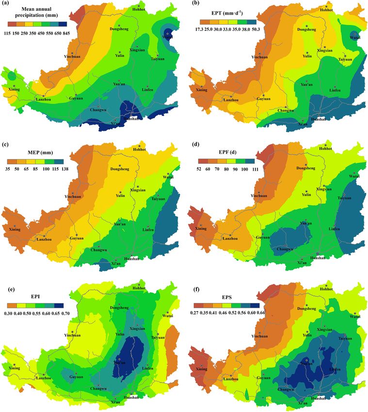
810             J. Zhang et al.: A universal multifractal approach to assessment of spatiotemporal extreme precipitation

EP has recently received increased attention (Eekhout et al.,        areas. Therefore, any investigation of spatiotemporal varia-
2018; Li et al., 2017; Wang et al., 2017). In this regard, there     tion in EP must make use of the information in the avail-
is a fundamental need to evaluate the regional spatiotempo-          able historical data that were observed at fixed time intervals
ral variation of EP, thereby providing important information         (e.g., daily). In EP assessment using historical daily data, it is
that is crucial for natural resource management and sustain-         a crucial step to identify EP events by extreme precipitation
able social development.                                             threshold (EPT) determination. However, EP events tend to
   The Loess Plateau (LP), which is located in the middle            be relatively rare, unpredictable, and often short-lived (Liu et
reaches of the Yellow River, is a typical arid and semi-             al., 2013); this uncertainty, combined with varying geograph-
arid region, characterized by serious EP-induced natural haz-        ical and meteorological conditions, increases the complexity
ards, including soil erosion and consequent hyperconcen-             of EP assessment.
trated flooding and occasional landslides (Cai, 2001). In the           In general, existing methods for EPT determination can
LP area, EP-induced soil erosion generates some of the high-         be grouped into two categories: nonparametric and paramet-
est sediment yields observed on Earth, ranging from 3 × 10⁴          ric. Nonparametric methods use fixed critical values or per-
to 4 × 10⁴ t km−2 yr−1 . For example, sediment delivered to          centiles to define the thresholds for extreme events. Because
the Yellow River in recent decades has been estimated to             the corresponding classification of EPTs varies from region
be 16 × 108 t yr−1 (Ran et al., 2000; Tang, 2004), and sed-          to region (e.g., a 50 mm daily precipitation event is consid-
iment deposition has resulted in the river bed of the lower          ered normal in South China but would be an EP event in
Yellow River aggrading by 8–10 m above the surrounding               the LP), the application of nonparametric methods can re-
floodplain (Shi and Shao, 2000). As the river flows on the ag-       quire considerable subjectivity (Liu et al., 2013) and signif-
graded thalweg, the extreme-precipitation-driven hypercon-           icantly affect the results of the analysis. For instance, using
centrated floodwaters cause the lower Yellow River to burst          an absolute value of 50 mm d−1 , Xin et al. (2009) reported a
its channel. Over the past 2500 years, this has caused 1593          spatiotemporal decreasing zone of EP in the central eastern
floods and 26 changes to the course of the river channel, lead-      LP, whereas, using the 95 % percentile to determine EP, Li et
ing to unimaginable death and devastation (Ren, 2006; Tang,          al. (2010a, b) found an increasing trend in the EP frequency
2004). To control such EP-induced natural hazards, ecologi-          in the southeastern LP. However, these reports did not explain
cal restoration projects have been implemented over the LP.          the rational for the spatial variation in EP and its impacts on
For example, the “Grain for Green” project (the largest in-          the most serious soil erosion in the central LP.
vestment project in China) was implemented to control nat-              Parametric statistical methods based on empirical distri-
ural hazards, such as soil erosion and flooding, and has cost        butions have recently become popular. A variety of special
more than USD 75 billion over the past 20 years.                     distribution functions and parameter estimation techniques
   Accordingly, a better understanding of spatiotemporal             have been proposed to characterize observed EP (Anagnos-
EP changes in this area is of considerable interest for vari-        topoulou and Tolika, 2012; Beguería et al., 2009; Deidda
ous fields, such as risk estimation, land management, flood          and Puliga, 2006; Dong et al., 2011; Li et al., 2005; Pfahl
control, and infrastructure planning (Feng et al., 2016; Wang        et al., 2017). A recent focus that has emerged is to ob-
et al., 2015). Considerable past work has been devoted to in-        tain a better physical understanding of EPTs and, thereby,
vestigating the spatiotemporal variation of total precipitation      to assess regional variations in EP. For example, Liu et
and precipitation extremes in this region, with a consensus          al. (2013) adopted a multifractal detrended fluctuation analy-
obtained with respect to precipitation “amount” (Li et al.,          sis (MFDFA) to determine EPTs, and Du et al. (2013) applied
2010a, b; Miao et al., 2016; Wan et al., 2014; Xin et al.,           MFDFA to investigate EPTs and consequent EP variation in
2009). However, the spatial distribution of EP in the LP is          northeastern China. To date, however, no international stan-
still poorly understood, with considerable disagreement re-          dards for the selection of such methods exist.
garding EP and the inability to account for the spatial dis-            Recent investigations of precipitation using the univer-
tribution of EP-induced hazards such as soil erosion (Li et          sal multifractal technique have demonstrated its multifractal
al., 2010a, b; Miao et al., 2016; Wan et al., 2014; Xin et al.,      nature. Universal multifractals were conceived to study the
2009). Thus, it is important to account for the spatiotemporal       multiplying cascades governing the dynamics of various geo-
role of EP in natural hazards in order to facilitate better catch-   physical fields (Lovejoy and Schertzer, 2013; Schertzer and
ment management with respect to issues such as freshwater            Lovejoy, 1987). For precipitation, a scaling break separating
shortage (Feng et al., 2012).                                        the meteorological and climatological regimes varies from
   To understand spatiotemporal variations in EP, scientists         several days to 1 month, with an average of about 2 weeks
are often required to collect more detailed data, including          (Tessier et al., 1993, 1994, 1996). The meteorological scal-
maximum depth, duration, and area observations (Dulière              ing interval indicates that (from the multifractal perspective)
et al., 2011; Herold et al., 2017; Miao et al., 2016). De-           data collected at time intervals of 1 d and those at intervals
spite sophisticated methodologies, such efforts rely on data         finer than minutes can equivalently characterize the physical
from various sources, which are typically absent in the long-        processes associated with precipitation (Pandey et al., 1998;
term historical observational records, especially over large         Tessier et al., 1996), indicating that EP events can, in prin-

Hydrol. Earth Syst. Sci., 24, 809–826, 2020                                         www.hydrol-earth-syst-sci.net/24/809/2020/
J. Zhang et al.: A universal multifractal approach to assessment of spatiotemporal extreme precipitation 811
ciple, be characterized by the study of daily data observed α 0
γ 1
at gauging stations. Of course, it is vitally important that the
C
1 C1 α 0 + α α 6= 1
c(γ ) = (4)
universal multifractal characterizes how extremes occur in a C exp γ − 1 α = 1,
1 C1
natural manner (Lovejoy and Schertzer, 2007; Tessier et al.,
1996).
where α is the multifractal index, which describes how
In this study, we use the universal multifractal technique to
rapidly the fractal dimensions vary as we leave the mean. For
obtain a physically meaningful characterization of EPT. Our
time series in this paper, 0 < α < 1, and α 0 is the auxiliary
objectives are to (1) apply the universal multifractal approach
variable defined by 1/α 0 + 1/α = 1 (Lovejoy and Schertzer,
to determine a unique set of EPTs for the LP area, (2) inves-
2013). The term C1 , the codimension of the mean of the pro-
tigate how spatial variations in EP are responsible for the se-
cess, varies as 0 ≤ C1 ≤ D (D is space dimension; D = 1
vere nature of soil erosion, and (3) assess the spatiotemporal
for time series) and quantifies the sparseness of the mean. In
variation of EP over the LP during the period from 1961 to
this paper, the parameters α and C1 of the multifractal model
2015.
were estimated using the double trace moment (DTM) tech-
nique (Lavallée et al., 1993).
2 Methodology As noted by Gagnon et al. (2006) and Lovejoy and
Schertzer (2007), the parameters C1 and α characterize the
2.1 The relationship between precipitation extremes mean of the field, whereas the extremes are expressed by the
and multifractals singularity, γ , and the codimension function c(γ ) (Hubert et
al., 1993). For 0 ≤ α < 1 and considering a time series of in-
The approach outlined below was used to identify EP events finite length, a finite maximum order of singularity, γ0 , can
at the observation timescale. In the method of universal mul- be determined as follows:
tifractals, two equivalent routes can be followed to investi-
gate time series scaling: the probability distribution and the C1
γ0 = . (5)
statistical moments. A fundamental property of multifractal 1−α
fields related to the probability distribution is given by the
However, in general, any time series of finite length will al-
following equation (Lovejoy and Schertzer, 2013; Schertzer
most surely miss the presence of rare extremes in the field.
and Lovejoy, 1987):
In this case, the observed singularities will be bounded by an
Pr ϕλ > λγ ≈ λ−c(γ ) ,
(1) effective maximum singularity, γs :
" −1/α 0 #
where λ represents the resolution of the measure (i.e., the C1
γs = γ0 1 − α < γ0 , (6)
ratio of the external scale L to the measurement scale l; D
λ = L/ l), ϕλ is the intensity of the field (in this case accumu-
lated precipitation) measured at resolution λ, γ is the order where D is the embedding space dimension (D = 1 for the
of singularity (maximum precipitation) corresponding to ϕλ , time series). The total dimension of this problem is actually
and the codimension function c(γ ) characterizes the sparse- (D + Ds ), where Ds = log Ns / log λ is the sampling dimen-
ness of the γ -order singularities (this function is a basic mul- sion, and Ns is the number of independent time series at each
tifractal probability relation for cascades). Accordingly, the location. The parameter γs links the physical processes that
statistical moments are given by generate precipitation events to the conceptual model of mul-
tiplicative cascades, and it allows the extremes to be cast in
q
ϕλ = λK(q) λ > 1, (2) a probabilistic framework, γs > 0. Thus, it was used to infer
the extreme events of precipitation fields over well-defined
where K(q) is the multiple scaling exponent function for mo- scales.
ments; q is the order of the statistical moment, and h i de- For parameter estimation, the parameters α and C1 of
notes the average of the field (averaged precipitation) at the multifractal model are estimated by the DTM technique
scale ratio λ. The two equivalent routes are related via a (Lavallée et al., 1993). The q, η DTM at resolution λ and 3
Legendre transform (Parisi and Frisch, 1985). The univer- is defined as
sal K(q) functions and the codimension function c(γ ) are q
expressed as * Z +
η q η D K(q,n)−(q−1)D
X
C T r λ ϕ3 = φ3 d x ∝ λ , (7)
1
(q α − q) α 6 = 1
K(q) = α−1 (3) i
Bλ,i
C1 q log(q) α=1
where the sum is obtained over all the disjoint D dimensional
balls Bλ,i (with intervals of length τ = T /λ) that are required
to cover the time series. K(q, η) is the double trace scaling
www.hydrol-earth-syst-sci.net/24/809/2020/ Hydrol. Earth Syst. Sci., 24, 809–826, 2020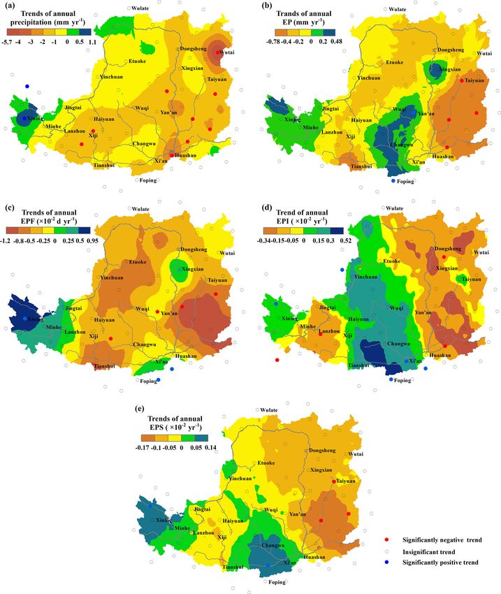
812            J. Zhang et al.: A universal multifractal approach to assessment of spatiotemporal extreme precipitation

exponent, and K(q, 1) = K(q) is the scaling exponent. This            EPT. The segmentation algorithm is based on the calculation
relation can be expressed as                                          of the statistic t of each data point in a series or subseries:
   η q                                                               τ = |(µL − µR ) /sD | ,                                   (11)
  ϕ3 λ = λK(q,n) ,                                     (8)
                                                                      where sD = [(sL2 +sR2 )/(NL +NR −2)]1/2 (1/NL +1/NR )1/2 is
where the notation indicates that the multifractal ϕ at a
                                                                      the pooled variance. The µL /µR , sL /sR , and NL /NR are the
(finest) resolution 3 is first raised to the power η then de-
                                                                      mean, standard deviation, and number of points from the data
graded to resolution λ, and the qth power of the result is aver-
                                                                      to the left/right of the series, respectively. The significance
aged over the available data. The scaling exponent K(q, η) is
                                                                      level P (τ ) of the largest value tmax obtained from Eq. (11)
related to K(q, 1) ≡ K(q) and is given by
                                                                      is defined as the probability of obtaining a value equal to or
K(q, η) = K(qη − 1) − qK(η, 1).                                (9)    less than τ within a random sequence (Swendsen and Wang,
                                                                      1987):
In the case of universal multifractals, by plugging Eq. (3) into
                                                                      P (τ ) = Pr {tmax ≤ τ } .                                 (12)
Eq. (9), K(q, η) has a particularly simple dependence on η:
                                                                      If the significance exceeds a selected threshold P0 (usually
K(q, η) = ηα K(q),                                            (10)    taken to be 95 %), an abrupt point is selected and the series
                                                                      is cut into two subsets at this point.
where α can be estimated from a simple plot of K(q, η) ver-              The pooled variances and the abrupt points of the α and
sus log(η) for fixed q. Thus, based on the DTM technique,             γs series are shown in Fig. 1b–d. The abrupt point, where
all parameters can be estimated.                                      sD differs from its left-side points but is approximately equal
                                                                      to its right-side points, is selected to be the EPT. As shown
2.2   Determination of the extreme precipitation
                                                                      for the determined EPT in Fig. 1, there is a steep slope of
      threshold
                                                                      the pooled variance on the left and a gentle slope on the right
The approach outlined below was used to estimate the EPTs             of 37.1 mm daily precipitation. Thus, the EPT for Xingxian
and EP events for each station, using the singularity parame-         station is estimated to be 37.1 mm d−1 , and 90 EP events have
ter (γs ). Given that the multifractal parameters α and γs nat-       occurred over the past 55 years (Fig. 1c).
urally characterize extremes, both of these parameters will
                                                                      2.3   EP indices
change if we gradually remove extreme values from the data
set. The singularity of the precipitation data series will be         All of the variables characterizing spatiotemporal EP over
completely changed, and the two parameters will signifi-              the LP are shown in Table 1. For individual stations, the
cantly change if all of the extreme values are deleted. To ob-        annual precipitation at each station was accumulated using
tain a physically meaningful value for the EPT, we attempted          daily data. Annual EP is accumulated using daily EP deter-
to estimate the multifractal parameter series by applying the         mined by the EPT, and EP frequency (EPF) is the number
universal multifractal approach to our precipitation series and       of daily EP events. Mean annual EP (MEP) is averaged from
successively eliminating maximum values of precipitation.             annual EP interpolated using ArcGIS 10.1. For a year with
However, as shown by Fig. 1a and c, the degree of conver-             n EP events, the EP intensity (EPI) is calculated by the fol-
gence of the original value is not unique, with the values fluc-      lowing equation:
tuating slightly around the original α and γs . Accordingly, the
                                                                                 n
variance series of index series αj and γs,j were computed to                  1X
eliminate the fluctuation while identifying the point of con-         EPI =         (EPi − EPT) /EPT, i = 1, 2, . . ., n,       (13)
                                                                              n i=1
vergence. The procedure is as follows:
                                                                      where EPi represents the magnitude of EP event i, respec-
 1. eliminate the data point xj , {xj , xj ≥ xmax −d ×j } from        tively.
    the precipitation time series {xi , i = 1, 2, . . . , n}, where      As noted by IPCC (2007), neither the cases of high fre-
    xmax is the maximum, xave is the average, and d is the            quency with low intensity nor the cases of low frequency
    interval space (we set d to 1 mm in this case);                   with high intensity can reflect the severity of EP events given
                                                                      a long-term time series for an area, whereas the severity
 2. compute the selected parameters;
                                                                      of EP (EPS) events relies on both intensity and frequency.
 3. repeat (1) and (2) for j varying from 1 to int((xmax −            Consequently, we examine the extreme precipitation inten-
    xave )/d).                                                        sity (EPI), extreme precipitation frequency (EPF, defined
                                                                      below), and EPS to characterize the spatiotemporal nature
Using the obtained parameter series, we applied the segmen-           of EP over the LP. To obtain the concordant EPS, each an-
tation algorithm proposed by Bernaola Galván et al. (2001) to         nual EPF/EPI series is standardized to the range from 0 to 1
determine the point of abrupt change, which we define as the          using Eq. (10):

Hydrol. Earth Syst. Sci., 24, 809–826, 2020                                           www.hydrol-earth-syst-sci.net/24/809/2020/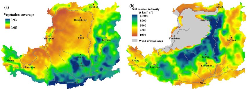
J. Zhang et al.: A universal multifractal approach to assessment of spatiotemporal extreme precipitation                                       813

Figure 1. Procedure for the EPT determination of the Xingxian station. (a) The multifractal index α (black dots) and the alternative abrupt
points (red dots). (b) Pooled variances (black dots) as calculated from the α series with the significant abrupt points (red dots) of the variances.
(c) As in panel (a) but for the singularity γS . (d) As in panel (b) but for the variance calculated from the γS series. (e) The time variation of
daily precipitation ranging from 1961 to 2015. The blue dotted line represents the determined EPT.

Table 1. Variables (abbreviations) used in this study addressing precipitation variations.

                 Abbreviation     Variables                                                                      Units
                 EPT              Extreme precipitation threshold                                                (mm d−1 )
                 MEP              Mean annual extreme precipitation                                              (mm)
                 EPF              Frequency of extreme precipitation event                                       (d)
                 EPI              Intensity of extreme precipitation event                                       (dimensionless)
                 EPS              Severity of extreme precipitation event                                        (dimensionless)
                 MDP              Long-term mean intra-annual daily precipitation                                (mm)
                 ADEP             Long-term accumulated intra-annual daily extreme precipitation events          (d)

www.hydrol-earth-syst-sci.net/24/809/2020/                                                    Hydrol. Earth Syst. Sci., 24, 809–826, 2020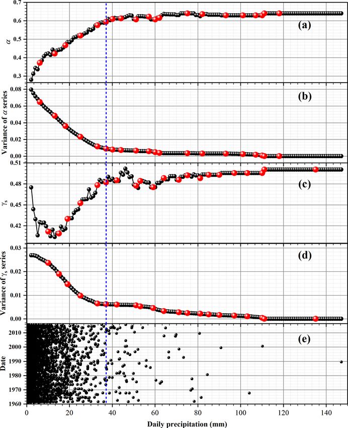
814 J. Zhang et al.: A universal multifractal approach to assessment of spatiotemporal extreme precipitation
100 to 300 m in thickness on the mountains, hills, basins, and
X = (Xi − Xmin ) / (Xmax − Xmin ) , (14) alluvial plains of different heights. The northwestern part of
the region is dominated by flat sandy areas. The middle and
where Xmin and Xmax represent the lowest and highest an- southeastern parts are characterized by EP-induced water-
nual EP frequency/intensity, respectively. The annual EPS erosion landforms (Zhang et al., 1997), with a rugged un-
for each station (0 ≤ EPS ≤ 1) is calculated from the stan- dulating ground surface that is broken, barren, and dissected
dardized EPI and EPF by by gullies and ravines (Cai, 2001). EP-induced flooding
episodes occur occasionally in the summer, with sediment
EPS = k1 PI + k2 PF , (15) concentrations generally exceeding 300 kg m−3 , although
they have been observed to be as large as 1240 kg m−3 . The
where k1 and k2 are the weight coefficients of frequency hyperconcentrated flooding has historically resulted in nu-
and intensity influencing EP severity, respectively, and k1 + merous disasters, with severe consequences for people and
k2 = 1. In this paper, k1 and k2 are set to 0.5 according to livestock (Zhang et al., 2017). The amount of soil erosion
IPCC (2007). has been estimated to be larger than 2 × 10⁹ to 3 × 10⁹ t yr−1
In addition, we compute the long-term mean daily pre- (Tang, 1990). Soil erosion has resulted in the density of gul-
cipitation (MDP) and the long-term accumulated daily lies and ravines in the LP being larger than 3–4 km km−2 ,
EP events (ADEP) to help characterize the intra-annual pre- with the maximum exceeding 10 km km−2 .
cipitation and EP. As shown in Table 1, MDP is averaged
from all 87 stations, and ADEP is accumulated from 87 sta- 3.2 Database
tions over the past 55 years.
To conduct the EP assessment, we used daily data that
2.4 Spatiotemporal EP presentation were available for 87 national meteorological stations in
and around the LP (Fig. 2), consisting of continuous time
The spatial distributions of the EP indices were derived by in- series from 1961 to 2015. All of the precipitation data
terpolation via kriging (Oliver and Webster, 1990), using data were obtained from the China Meteorological Data Sharing
observed at the gauging stations. All spatial analyses were Service System (http://data.cma.cn/, last access: 19 Febru-
carried out using the ArcGIS 10.1 software. Spatiotemporal ary 2020). Missing data accounted for less than 0.1 % of the
trends for annual EP indices were computed for each pixel total sample, and they were replaced by a value of zero in
using the least squares method. Following Stow et al. (2003), this paper; this replacement of a few missing values does
the trend is defined as the slope of the least squares line that not influence the analysis. Data regarding the severity of
fits the inter-annual variability of individual EP indices dur- soil erosion were provided by the LP Science Data Cen-
ing the study period and is given by ter of the data sharing infrastructure of the National Earth
! ! System Science Data Center of China (http://loess.geodata.
m m m
P P P cn, last access: 19 February 2020). These data were com-
m× j × Pj − j Pj
j =1 j =1 j =1 piled during the Soil Erosion Census of the China Census
S= !2 , (16) for Water (Ministry of Water Resources and National Bu-
m m
m×
P
j2 −
P
j reau of Statistics, 2013). Mean annual vegetation coverage
j =1 j =1 at an 8 km spatial resolution and a 15 d temporal resolu-
tion were computed using data for the period from 1982
where m is the total of years, and Pi is value of the pixel in to 2006, which were produced by the Global Inventory
the j -th year. Modeling and Mapping Studies (GIMMS) group from mea-
surements of the Advanced Very-High-Resolution Radiome-
ter (AVHRR) onboard the NOAA 7, NOAA 9, NOAA 11,
3 Study area and database and NOAA 14 satellites. Data from the National Center for
Environmental Prediction/National Center for Atmospheric
3.1 Study area
Research (NCEP/NCAR) Reanalysis Project (Kalnay et al.,
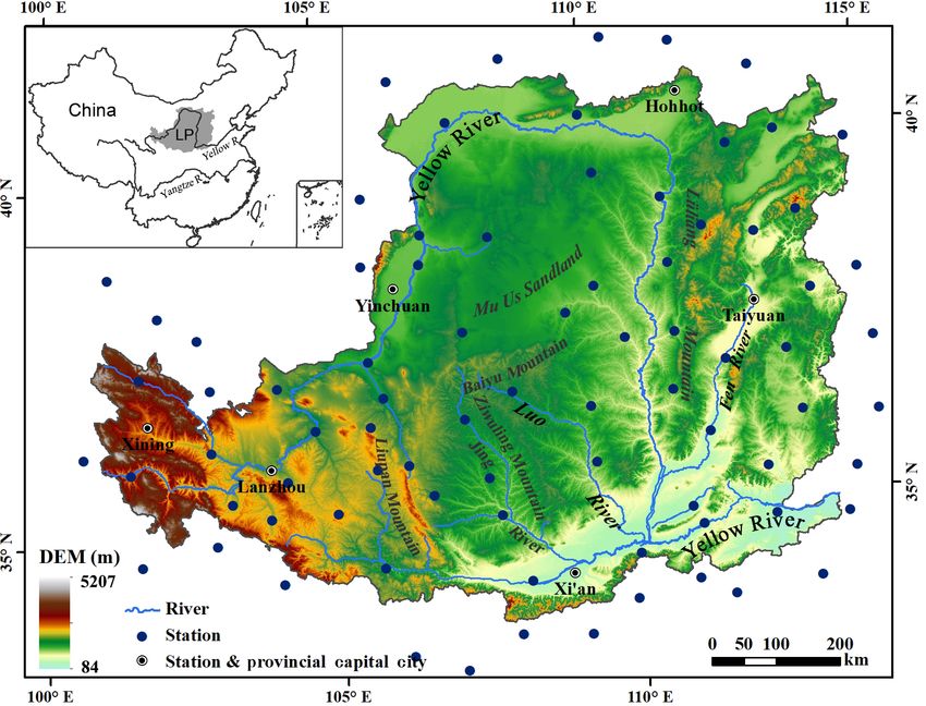
The LP (640 000 km2 ) is a typical arid and semiarid 1996) were also used in this study. The variables selected
area located in the middle reaches of the Yellow River for analysis were the monthly mean geopotential height,
(750 000 km2 ) and is characterized by a continental mon- monthly mean wind, daily mean sea level pressure, and
soon climate. Elevations range from 84 to 5207 m (Fig. 2). daily mean wind from 1961 to 2013 on a 2.5◦ × 2.5◦ spatial
The desert steppe, typical steppe, and forest steppe (decid- grid (http://www.esrl.noaa.gov/psd/, last access: 19 Febru-
uous broadleaf forest) zones are distributed from northwest ary 2020).
to southeast and correspond to mean annual isohyets of 250,
450, and 550 mm in the arid, semiarid, and semi-humid ar-
eas, respectively. The continuous loess covering ranges from
Hydrol. Earth Syst. Sci., 24, 809–826, 2020 www.hydrol-earth-syst-sci.net/24/809/2020/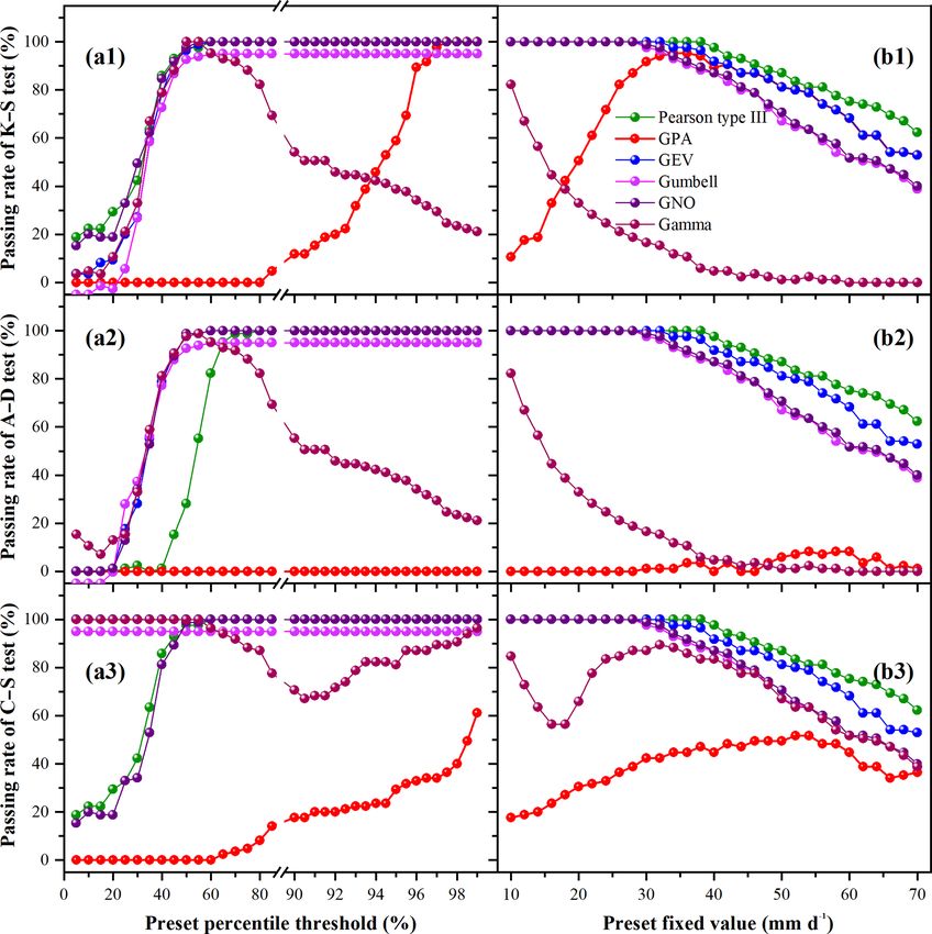
J. Zhang et al.: A universal multifractal approach to assessment of spatiotemporal extreme precipitation                               815

Figure 2. Location of the Loess Plateau in the middle reaches of the Yellow River, China (inset), and the distribution of the meteorological
stations in and around the LP.

4     Results                                                           contrast with each other, with the highest EPIs centered in
                                                                        the mid-eastern LP, where EPFs were comparatively lower,
4.1    Spatial characteristics of extreme precipitation                 and the lowest EPIs centered in the southeastern LP, which
                                                                        had the maximum mean annual precipitation and EPF. The
Figure 3a shows that the mean annual precipitation (for the             highest values of EPI dominated the central LP area. The
period from 1961 to 2015) varied from 115 mm in the north-              northern boundary of the area was positioned southeast of
western LP to the 845 mm in the southeastern LP. The as-                the Mu Us Desert (Dongsheng and Xingxian); the west-
sociated EPTs ranged from 17 mm d−1 in the northwest to                 ern boundary was positioned west of the Liupan Moun-
50 mm d−1 in the southeast (Fig. 3b); these EPT isohyets are            tains (Guyuan County); the eastern boundary was positioned
generally consistent with those of mean annual precipitation.           northeast of the Lüliang Mountains and the Fenhe Valley
Figure 3b indicates that the area around the Dongsheng sta-             (Taiyuan and Linfen); the southern boundary was positioned
tion is a regional EP center: the EPTs around the station are           to the north of the central Shaanxi Plain (Huashan, Xi’an and
higher than those of the surrounding areas, whereas the iso-            Changwu). The EPI presents the event EP power causing nat-
hyets of mean annual precipitation are smooth. The spatial              ural hazards. This high value of EPI partially explains why
distribution of MEP is also similar to that of mean annual pre-         this area is characterized by very serious soil erosion that re-
cipitation, increasing from northwest to southeast and rang-            leases more than 2 × 10⁹ t of sediment into channels of the
ing from 35 to 138 mm yr−1 (as shown in Fig. 3c). MEP max-              Yellow River annually.
imums occur in the southern and southeastern LP.                           Figure 3f indicates that the spatial distribution of EPS in
   Figure 3d indicates that EPFs have ranged from 54 to 115 d           the LP increased from the northwest to the southeast, rang-
(i.e., mean annual EPF ranged from 1.0 to 2.1 d) over the               ing from 0.27 to 0.66, but the highest EPSs were centered
region during the past 5 decades. Notable occurrences of                in the southeast central LP. The areas with the highest EPSs
high EPF can be seen in and around the Ziwuling Mountains               covered the basins of the Jing, Luo, and Fen rivers. Although
in the mid-southern LP, whereas the highest frequency oc-               EP events always occurred over a small range, the spatial
curred to the east of the Fenhe Valley in the southeastern LP.          maps of EPI, EPF, and EPS indicate that the areas with seri-
Meanwhile, the lowest frequency occurred in the northwest-              ous EP events are regularly distributed.
ern LP, the western Mu Us sandy land, and the western Liu-
pan Mountains.
   Figure 3e indicates that the averaged EPIs mainly ranged
between 0.3 and 0.7. The spatial variations in EPI and EPF

www.hydrol-earth-syst-sci.net/24/809/2020/                                               Hydrol. Earth Syst. Sci., 24, 809–826, 2020
816 J. Zhang et al.: A universal multifractal approach to assessment of spatiotemporal extreme precipitation
Figure 3. Spatial distributions of (a) mean annual precipitation, (b) EPTs, (c) MEP, (d) total EPF, (e) mean EPI, and (f) mean annual EPS in
the LP from 1961 to 2015.
4.2 Spatiotemporal variation of EP in the annual EP ranged from −0.78 to +0.48 mm yr−1
(Fig. 4b), with 23.8 % of the total area showing a posi-
Our results (Fig. 4a) indicate that 91.4 % of the LP was char- tive trend and increased annual EP distributed mainly in the
acterized by a negative annual precipitation trend over the southwestern LP (west of Lanzhou) and the central south-
study period, whereas only 8.6 % of the total area presented ern LP (Beiluo and Jing river basins and an area around the
a positive trend. A total of 9 out of 87 stations showed a sig- Xingxian station). Meanwhile, the annual EPF has changed
nificant negative trend, whereas 2 stations showed positive by −0.6 to +0.5 d over the past 55 years, with a change rate
trends (p < 0.1). At the same time, the spatiotemporal trends
Hydrol. Earth Syst. Sci., 24, 809–826, 2020 www.hydrol-earth-syst-sci.net/24/809/2020/J. Zhang et al.: A universal multifractal approach to assessment of spatiotemporal extreme precipitation 817
ranging from −1.2×10⁻² to +0.95×10⁻² d yr−1 (as shown cipitation from June to September accounts for 72 % of the
in Fig. 4c). Of the 87 stations, 4 stations showed a significant total amount, while 91 % of the total EP events occur from
negative trend in EPF, whereas 3 stations showed positive June to August. According to the fitted curve (Fig. 5), the
trends (p < 0.1). The areas with a negatively trending EPF highest MDP occurred on 26 July, which is 11 d earlier
covered 86.4 % of the total area, whereas the areas with posi- than the maximum ADEP on 6 August. Based on fitting the
tively trending EPF covered 13.6 %; the latter regions mainly four-parameter Weibull curve (p < 0.0001), the MDP for the
occurred in the southwestern LP (around the Xining station) 224 d from 26 March to 4 November accounted for 95 % of
and in the areas around the Xi’an and Xingxian stations. The the mean annual precipitation. Meanwhile, the ADEP from
areas with notably decreasing trends mainly occurred in the 21 May to 18 September accounted for 95 % of the total EPF.
central western and southeastern regions of the LP. Therefore, the high concentration of the amount of daily
Figure 4d indicates that the changes in annual EPI ranged precipitation into a limited period results in a significant al-
from −0.18 to +0.27, with a changing rate ranging from ternation of wet and dry seasons in the LP. In addition, low
−0.34 × 10⁻² to 0.52 × 10⁻² yr−1 . We found that 34 of the precipitation, the annual alteration of dry and wet seasons,
87 stations showed upward slopes (5 stations with a signif- and highly concentrated intra-annual EP events with an oc-
icance level of p < 0.1), and 53 stations showed negative currence 11 d earlier than the wettest days contribute to a
slopes (4 stations with a significance level of p < 0.1). As fragile eco-environment subject to severe natural hazards.
shown in Fig. 4d, areas with positive trends in EPI accounted Specifically, lower precipitation coupled with the occurrence
for 42.2 % of the total area, with the areas delineated by the of the highest EPI and EPS are responsible for the most se-
Wulate, Yan’an, and Huashan stations and the Jingtai, Xiji, vere hazard situations in the central LP, such as soil erosion.
and Tianshui stations as well as the area west of the Minhe
station. The areas with a negative slope covered 57.8 % of the 4.3.2 Atmospheric circulation factors for the spatial
total area. variation of extreme precipitation
Figure 4e indicates that the annual EPSs changed
by −0.09 to +0.07 during the study period, with rates vary- Atmospheric circulation is the leading factor causing the
ing from −0.34 × 10⁻² to 0.52 × 10⁻² yr−1 . Of the 87 sta- abovementioned phenomena. The LP is located in the East
tions, 39 stations showed a positive slope (3 stations with Asian monsoon region. According to the average sea level
a significance level of p < 0.05), while 54 stations exhib- pressure and winds in winter from 1961 to 2015 (see Fig. 6a),
ited a negative slope (2 station with a significance level of the dry winter in the region is influenced by the interactions
p < 0.05). The areas with increased EPSs covered 25.4 % of between two high-pressure areas in southwestern China (the
the total area and were mainly found in an area delineated by Tibet Plateau high-pressure system) and North China (the
the Wuqi, Tianshui, and Huashan stations and an area west Mongolian high-pressure system). The prevailing East Asian
of the Xiji station. The areas with negative trends accounted winter monsoon (which has a north-northwest direction) cir-
for 74.6 % of the total area. culates in East China and brings cold and dry airstreams. In
The trend estimates computed for annual EP, EPF, and EPI contrast, the summer climate of the LP is affected by inter-
are associated with strong uncertainty. For instance, the up- actions between two high-pressure systems, the Pacific high-
ward trend in annual EP in and around the Xingxian station pressure system and the Tibet Plateau high-pressure system.
relied heavily on the upward trend in the EPF and not the Figure 6b shows that the prevailing East Asian summer mon-
downward trend in the EPI. The EPF around the Changwu soon (which has a south-southeast wind direction) brings
station decreased, but both the annual EP and EPS increased warm and humid maritime airstreams that spread from the
with the upward trend in the EPI. However, nearly all of the West Pacific to central China. However, the Tibet Plateau
areas with positive trends for annual EP, EPI, EPF, and EPS high-pressure system has a notable effect on the climate of
had a negative trend in annual precipitation (Fig. 4). It should the northwestern LP, and the airstream humidity decreases
be noted that 62.1 % of the LP area with a negative trend in gradually as the distance from the Pacific increases. The re-
annual precipitation has more than one EP indices with pos- sulting effect and decreased humidity form a vast arid region
itive trends, potentially indicating the risk of more serious in northwestern China, including the northwestern LP, with a
hazardous situations. prevailing west-southwest wind direction. This explains why
precipitation decreases from the southeast to the northwest,
4.3 Intra-annual EP characteristics and their and precipitation is scarce in the northwestern LP.
relationship with large-scale atmospheric Nevertheless, tropical cyclones occasionally enter the cen-
circulation tral LP, accompanied by EP events. For instance, in Au-
gust 1996 a western Pacific cyclone landed in the southeast-
4.3.1 The intra-annual distribution of EP events ern coastal area of China and weakened gradually as it moved
northwest, as shown by the 1000 hPa geopotential height and
Figure 5 displays the intra-annual distributions of the MDP winds in Fig. 6c. Plenty of rainstorms or intense rainfall
and the ADEP for the 87 stations from 1961 to 2015. Pre- events that accompanied the cyclone occurred in its transit
www.hydrol-earth-syst-sci.net/24/809/2020/ Hydrol. Earth Syst. Sci., 24, 809–826, 2020818 J. Zhang et al.: A universal multifractal approach to assessment of spatiotemporal extreme precipitation Figure 4. The spatial distribution of the trends and the stations with significant trends (p < 0.1) for (a) annual precipitation, (b) annual EP, (c) annual EPF, (d) annual EPI, and (e) annual EPS in the LP from 1961 to 2015. area. On 3 August 1996, the weakened cyclone reached the as shown in Fig. 6d, the cyclone was blocked from entering southeastern LP (as shown in Fig. 6d). However, due to the the northwestern LP, moved towards the northeast, and grad- control of the Tibet Plateau high-pressure system, the cen- ually dissipated. These phenomena illustrate why this region tral LP is generally the northwestern inland boundary with has limited precipitation but severe EP events. respect to the reach and impact of tropical cyclones. Thus, Hydrol. Earth Syst. Sci., 24, 809–826, 2020 www.hydrol-earth-syst-sci.net/24/809/2020/
J. Zhang et al.: A universal multifractal approach to assessment of spatiotemporal extreme precipitation                            819

Figure 5. Intra-annual distribution of daily precipitation (MDP) and the number of daily EP events (ADEP) for the 87 stations from 1961
to 2015 and their fitting curves with respect to a Weibull function.

Figure 6. Average sea level pressure and winds: (a) the mean for all winters (from December to February) and (b) the mean for all summers
(from June to August) from 1961 to 2015. Characteristics of the average 1000 hPa geopotential height and winds on (c) 1 August 1996 and
(d) 3 August 1996. The data were derived from global NCEP/NCAR reanalysis average monthly and daily data.

www.hydrol-earth-syst-sci.net/24/809/2020/                                             Hydrol. Earth Syst. Sci., 24, 809–826, 2020
820             J. Zhang et al.: A universal multifractal approach to assessment of spatiotemporal extreme precipitation

Figure 7. (a) Spatial distribution of mean vegetation coverage in summer (from June to August) on the Loess Plateau from 1982 to 2006 at
a spatial resolution of 8 km. (b) Spatial distribution of the soil erosion intensity, which was resampled to a spatial resolution of 8 km.

5     Discussion                                                          Zhou and Wang (1992) divided the LP into three zones
                                                                       of raindrop kinetic energy (< 1000, 1000–1500, and 1500–
5.1    Rationality of spatial EP characteristics                       2000 J m−2 yr−1 , respectively), based on observations of the
                                                                       raindrop kinetic energies of rainstorms during 1980s. We
Natural hazards related to EP can be divided into two cate-            found that the 30 and 35 mm d−1 EPT contours closely over-
gories: (1) hazards accompanied by EP and (2) hazards that             lap with the raindrop kinetic energy contours of 1000 and
follow the occurrence of EP. For the former, one focus is              1500 J m−2 yr−1 . Further, soil erosion in the LP in re-
the dependence between EP and storm surges in the coastal              cent decades has been found to be approximately 5000–
zone. Using such dependence structures, EP and storm surges            10 000 t km−2 yr−1 (Ludwig and Probst, 1998; Shi and Shao,
can be quantified to provide information for successful haz-           2000). Such high rates of sediment erosion are generally in-
ard management (Svensson and Jones, 2004; Zheng et al.,                duced by several rainstorm events during the year, with the
2013). For the latter, the LP is such that the area suffers from       top five daily sediment yields accounting for 70 %–90 % of
EP-induced natural hazards that exceed the general tolerance           the annual total soil loss (Rustomji et al., 2008; Zhang et
of the natural environment, existing ecosystems, human life,           al., 2017). For instance, a 200-year precipitation event in
and the social economy. In this case, the rational characteris-        Wuqi on 30 August 1994 induced a flooding event with a
tics of EP responsible for spatial hazards can be studied.             daily sediment concentration of 1060 kg m−3 . The stream-
   Here, we use the widely distributed soil erosion to verify          flow was 2.41 times the mean annual streamflow from 2002
the rationality of our results. According to the universal soil        to 2011, and the sediment load was equivalent to 9.6 % of
loss equation (Wischmeier, 1976), the rational characteris-            the total sediment yields from 1963 to 2011 (Zhang et al.,
tics of EP should correlate well with soil erosion and vege-           2016). Therefore, the EPF obtained in this study, about twice
tation coverage (Fig. 7). To examine this, partial correlation         every year on average, is rational to explain such serious
analyses were performed between soil erosion intensity and             sediment erosion. In the LP, spring drought is the limiting
EPI/EPS as well as with the vegetation coverage. Our results           factor with respect to vegetation (especially herbaceous veg-
indicate that water-based erosion intensity correlates signif-         etation) recovery from winter every year, and grass gener-
icantly with vegetation coverage (negatively, Fig. 7a) and             ally germinates on an extensive scale after the first effective
EPS (positively, Fig. 3f); the related coefficients are −0.61          rainfall event (> 5 mm) in spring (Cai, 2001; Tang, 1993,
(p < 0.001) and 0.53 (p < 0.001), respectively. For the cor-           2004). However, as shown in Fig. 5, the highest EPF occurred
relations between water-erosion intensity and vegetation cov-          11 d earlier than the day of maximum daily precipitation in
erage as well as with EPI (Fig. 3e), the coefficients are −0.58        the LP. This means that the days on which the LP experiences
(p < 0.001) and 0.76 (p < 0.001), respectively. This find-             most serious EP events tend to be days when precipitation is
ing demonstrates the rationality of our results. Note that, the        low. In other words, every year, the vegetation has not suffi-
higher correlation between EPI and soil erosion agrees with            ciently recovered when frequent EP events occur in the LP.
the results of plot experiments by Tang (1993), who noted              Such an intra-annual distribution of precipitation is one of
that high-intensity precipitation is the primary driving force         the climatic reasons why there is serious soil erosion in the
of erosion.                                                            semiarid LP. Further, the sparse spatial nature of precipita-
                                                                       tion is insufficient for the growth of high-coverage vegeta-

Hydrol. Earth Syst. Sci., 24, 809–826, 2020                                            www.hydrol-earth-syst-sci.net/24/809/2020/
J. Zhang et al.: A universal multifractal approach to assessment of spatiotemporal extreme precipitation 821
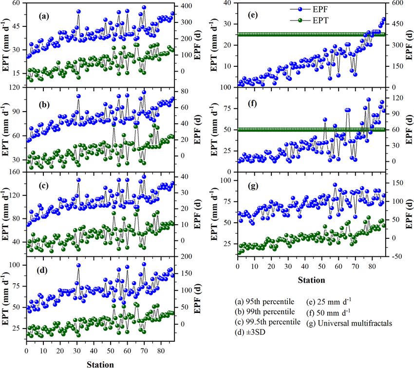
Figure 8. EPTs determined by different methods and the corresponding EP frequencies for 87 stations over the Loess Plateau. The abscissa
represents the stations with an increase in the mean annual precipitation from 104 to 918 mm.
tion, especially in the northwestern LP (Fig. 7a). However, precipitation events are relatively rare, poorly predictable,
the highest EPI provides the strongest erosion force, which and often short-lived, resulting in uncertainty in EP event
contributes to the severe rates of erosion (Fig. 7b) in the cen- identification. The uncertainties regarding EPT determina-
tral LP. Thus, these results regarding the EP responsible for tion from parametric and nonparametric methods has been
hazardous situations (both spatially and temporally) are im- discussed in Sect. 2.
portant for sustainable catchment management, ecosystem Figure 8 shows the results of the EPF obtained using non-
restoration, and water resource planning and management parametric methods for all 87 stations over the LP during the
within the LP. Given that 62.1 % of the total LP with a nega- period from 1961 to 2015. Large variances among the re-
tive trend in annual precipitation has one or more positive EP sults, calculated at different percentile levels, are shown in
indices, the underlying upward trends in water erosion and Fig. 8a–c. Trivially, the EPTs are smaller but with larger
sediment yield should be taken into account in catchment EPFs for lower percentiles. The “±3 SD (standard devia-
management efforts. tion)” method (Fig. 8d) provided results with a similar vari-
ance among stations in comparison with the universal mul-
5.2 Uncertainty in EP identification tifractal method (Fig. 8g). The EPTs determined by indi-
vidual methods generally increase as annual precipitation
The uncertainties in the identification and assessment of EP increases. As shown in Figs. 8e–f and 3a, no precipitation
events stem from two aspects: (1) the stochasticity in climate event exceeded 50 mm d−1 , as the mean annual precipitation
(Miao et al., 2019) and (2) the methodology (Papalexiou et is < 200 mm in the northwestern LP. A 50 mm d−1 threshold
al., 2013). For the former, significant spatiotemporal varia- is probably suitable for the southeast LP, which has higher
tions occur in EP events as a result of varying geographical mean annual precipitation, whereas a 25 mm d−1 threshold
and meteorological conditions (Pinya et al., 2015). Extreme
www.hydrol-earth-syst-sci.net/24/809/2020/ Hydrol. Earth Syst. Sci., 24, 809–826, 2020822 J. Zhang et al.: A universal multifractal approach to assessment of spatiotemporal extreme precipitation
may be more suitable for some stations in the northwest- Table 2. Passing rates of the goodness-of-fit test for EP events de-
ern LP. Therefore, regardless of the varying geographical and termined using the universal multifractals method.
meteorological conditions, the selection of these thresholds
can be quite subjective and empirical. Note that, although Function K–S A–D C–S
a similar variance of EPTs among stations can be obtained test test test
using individual methods, the spatial causes for hazards situ- (%) (%) (%)
ations cannot be theoretically explained by these methods in Gamma 100 100 100
Fig. 8a–f. GPA 100 100 100
Parametric methods require a predetermined threshold Gumbell 100 100 100
value, above which the data can be chosen as the EP series Pearson type III 100 100 100
if the data series passed the goodness-of-fit test. As shown GEV 100 100 100
in Fig. 9, both fixed values and percentiles were adopted GNO 100 100 100
to preset EPT. The selected rainfall data series were fit-
ted to the gamma, GPA (generalized Pareto distribution),
Gumbel, Pearson type III, GEV (generalized extreme value As noted by Pandey et al. (1998) and Douglas and Bar-
distribution), and the GNO (generalized normal) distribu- ros (2003), these methodological uncertainties arise due to
tions, whose parameters were estimated utilizing the L- the wide gap between mathematical modeling and the phys-
moments method (Haddad et al., 2011) at a 0.05 signif- ical understanding of precipitation processes. As previously
icance level, using goodness-of-fit tests including the K– mentioned, the multifractal technique can be used to describe
S (Kolmogorov–Smirnov test), A–D (Anderson–Darling K- the statistical probability and physical processes associated
Sample test) and C–S (Pearson’s Chi-squared test) tests. As with observed data (Lovejoy and Schertzer, 2013; Tessier et
shown in Fig. 9a1–a3 and b1–b3, the results of the three tests al., 1996), while the scale invariance of multifractals enables
are similar, although they differ with respect to the details for the multifractal technique to also overcome the influence of
the preset fixed value and percentile thresholds. the sample size (Pandey et al., 1998; Tessier et al., 1996).
Further, these results for different distribution functions Further, the segmentation algorithm helps to overcome the
are quite different from each other. As shown in Fig. 9a1 problem of uncertainty. In the present study, the general cor-
and a2 (by the K–S and A–D tests), the passing rates from respondence and the specific divergences between the EPT
the GEV, Gumbell, GNO, and Pearson type III distribution and precipitation isohyets (Fig. 3) further exhibits the varying
functions are high, whereas there are very low passing rates meteorological and geographical influences. As shown in Ta-
from the GPA and Gamma functions. In addition, the passing ble 2, by fitting EP series derived using universal multifrac-
rates are different between the preset methods of percentiles tals to the six distribution functions, the 100 % passing rate
and fixed values. As shown in Fig. 9, the GEV and Gum- of the goodness-fit test strongly supports that the universal
bell distribution function have high passing rates for EP se- multifractal approach is advanced in identifying EP events.
ries obtained by preset percentiles when the percentile is less Overall, the universal multifractal method provides a much
than or equal to 99 % (Fig. 9a1, a2), whereas the passing superior approach to addressing uncertainties and providing
rates for the series obtained using fixed values decrease with a unique set of EPTs.
increasing values (Fig. 9b1, b2). We also found that these
distribution functions are not sensitive to the percentile or
fixed value changes. These findings indicates that the fitting 6 Conclusions
accuracy can be greatly affected by the selection of the ex-
treme value distribution functions, the goodness-of-fit tests, Using data from 87 meteorological stations from 1961
and the methods used for the EPT preset. Liu et al. (2013) to 2015, we have proposed an approach that integrates uni-
noted that the fitting accuracy is also affected by the size of versal multifractals with a segmentation algorithm to enable
rainfall series. Thus, unavoidably, applications of paramet- the identification of EP events and, thereby, to assess the spa-
ric methods also depend on personal subjectivity and em- tiotemporal EP characteristics in the LP. We find that the spa-
piricism. We have attempted to explore EP using fixed val- tial distribution of the EPTs increased from 17.3 mm d−1 in
ues of spatiotemporal variation in precipitation analysis in the northwestern LP to 50.3 mm d−1 in the southeastern LP.
the LP; however, we found that the results did not explain the Similarly, the MEP increased from 35 mm to 138 mm yr−1 ,
rainfall-induced natural hazards well nor did they agree (spa- with the maximum MEP occurring in the southern and south-
tially) with plot experiments by Wan et al. (2014) or results eastern LP. The EPF over the LP has been within a range
obtained using fixed values (Xin et al., 2009) and percentiles of 54–116 d over the last 55 years. Notable occurrences of
(Li et al., 2010a, b). These uncertainties may be the reason EPFs have mainly been observed in the central southern and
why prior EP studies over the LP tend to disagree with each southeastern LP. An examination of atmospheric circulation
other. patterns demonstrates that the central LP is the inland bound-
ary with respect to the reach and impact of tropical cyclones
Hydrol. Earth Syst. Sci., 24, 809–826, 2020 www.hydrol-earth-syst-sci.net/24/809/2020/J. Zhang et al.: A universal multifractal approach to assessment of spatiotemporal extreme precipitation 823 Figure 9. The passing rates of the goodness-of-fit test for individual distribution functions, with EP data series selected by different preset thresholds. (a1) The K–S test, (a2) the A–D test, and (a3) the C–S test for different distribution functions using preset percentile thresholds. (b1) The K–S test, (b2) the A–D test, and (b3) the C–S test for different distribution functions using thresholds of fixed values. The sig- nificance level is 0.05. The symbol lines of the passing rate of Gumbell functions in (a1)–(a3) were arbitrarily offset upward by −5 units, respectively, in order to separate them. in China; therefore, the highest EP intensity and EP sever- 23.8 %, 13.6 %, 42.2 %, and 25.4 % of the LP area, respec- ity are found in this area. Correlation analysis significantly tively. It should be noted that 62.1 % of the LP area with neg- supported the reasonability of the spatial estimates of the ative annual precipitation experienced upward trends in one EP characteristics that are responsible for hazardous situa- or more of the EP variables. It can be concluded that EP over tions over the LP. The climate factors for the most serious the LP intensified, potentially imposing a risk of more seri- hazardous situations in the LP, especially in the central LP, ous hazardous situation. Sustainable countermeasures should stem from the low precipitation, the highest EPI, and the high be considered in the catchment management to address the ADEPs that are concentrated 11 d earlier than the wet season. underlying hazards. Spatiotemporally, annual EP increased in the southwest- In conclusion, the universal multifractal approach consid- ern and central southern LP. Areas with a positive EPF trend ers both the physical processes and their probability distribu- were found in the southwestern LP as well as the regions tion and, thereby, provides an approach to overcome uncer- around the Xi’an and Xingxian stations, whereas areas with tainties and identify EP events without the need for empirical a positive trend in EPI occurred among the Wulate, Yulin, adjustments. Thus, this approach is useful for application to Yan’an, and Huashan stations and the Jingtai, Xiji, and Tian- spatiotemporal EP assessment at the regional scale. shui stations, as well as the region west of the Minhe station. The annual EPSs (with increased slope) covered an area de- lineated by the Wuqi, Tianshui, and Huashan stations and an Data availability. All of the data used in this study are available area west of the Xiji station. Overall, the areas with upward upon request. trends in the annual EP, EPF, EPI, and EPS accounted for www.hydrol-earth-syst-sci.net/24/809/2020/ Hydrol. Earth Syst. Sci., 24, 809–826, 2020
824              J. Zhang et al.: A universal multifractal approach to assessment of spatiotemporal extreme precipitation

Author contributions. JZ, XZ, and RL prepared the research                 world’s dry and wet regions, Nat. Clim. Change, 6, 508–513,
project. JZ, HVG, GG, BF, and CW conceptualized the methodol-              https://doi.org/10.1038/NCLIMATE2941, 2016.
ogy. JZ developed the code and performed the analysis. JZ prepared       Dong, Q., Chen, X., and Chen, T.: Characteristics and Changes
the paper with contributions from all the co-authors.                      of Extreme Precipitation in the Yellow–Huaihe and Yangtze–
                                                                           Huaihe Rivers Basins, China, J. Climate, 24, 3781–3795, 2011.
                                                                         Douglas, E. M. and Barros, A. P.: Probable maximum precipitation
Competing interests. The authors declare that they have no conflict        estimation using multifractals: application in the Eastern United
of interest.                                                               States, J. Hydrometeorol., 4, 1012–1024, 2003.
                                                                         Du, H., Wu, Z., Zong, S., Meng, X., and Wang, L.: Assessing the
                                                                           characteristics of extreme precipitation over Northeast China us-
Acknowledgements. We thank the China Meteorological Data Shar-             ing the multifractal detrended fluctuation analysis, J. Geophys.
ing Service System, the Yellow River Conservancy Commission,               Res.-Atmos., 118, 52013, https://doi.org/10.1002/jgrd.50487,
the LP Science Data Center of the data sharing infrastructure of           2013.
the National Earth System Science Data Center of China, and the          Dulière, V., Zhang, Y., and Salathé Jr, E. P.: Extreme precipitation
NCEP/NCAR for providing data used in this paper. All data sources          and temperature over the US Pacific Northwest: A comparison
are publicly accessible, and these websites are listed in Sect. 3.2.       between observations, reanalysis data, and regional models, J.
                                                                           Climate, 24, 1950–1964, 2011.
                                                                         Eekhout, J. P. C., Hunink, J. E., Terink, W., and de Vente, J.: Why
                                                                           increased extreme precipitation under climate change negatively
Financial support. This research was funded by the National
                                                                           affects water security, Hydrol. Earth Syst. Sci., 22, 5935–5946,
Natural Science Foundation of China (grant nos. 41701207
                                                                           https://doi.org/10.5194/hess-22-5935-2018, 2018.
and 41822103), the State Key Project of Research and Develop-
                                                                         Feng, X. M., Sun, G., Fu, B. J., Su, C. H., Liu, Y., and Lamparski,
ment Plan of China (grant no. 2016YFC0501603), the Open Foun-
                                                                           H.: Regional effects of vegetation restoration on water yield
dation of the State Key Laboratory of Urban and Regional Ecol-
                                                                           across the Loess Plateau, China, Hydrol. Earth Syst. Sci., 16,
ogy of China (grant no. SKLURE2019-2-5), and the Fundamen-
                                                                           2617–2628, https://doi.org/10.5194/hess-16-2617-2012, 2012.
tal Research Funds for the Central Universities of China (grant
                                                                         Feng, X., Fu, B., Piao, S., Wang, S., Ciais, P., Zeng, Z., Lü, Y.,
no. 2652018034). The corresponding author acknowledges partial
                                                                           Zeng, Y., Li, Y., and Jiang, X.: Revegetation in China’s Loess
support from the Australian Centre of Excellence for Climate Sys-
                                                                           Plateau is approaching sustainable water resource limits, Nat.
tem Science (grant no. CE110001028).
                                                                           Clim. Change, 6, 1019–1022, 2016.
                                                                         Gagnon, J.-S., Lovejoy, S., and Schertzer, D.: Multifractal
                                                                           earth topography, Nonlin. Processes Geophys., 13, 541–570,
Review statement. This paper was edited by Nadia Ursino and re-            https://doi.org/10.5194/npg-13-541-2006, 2006.
viewed by three anonymous referees.                                      Haddad, K., Rahman, A., and Green, J.: Design rainfall estimation
                                                                           in Australia: a case study using L moments and generalized least
                                                                           squares regression, Stoch. Environ. Res. Risk A., 25, 815–825,
                                                                           2011.
                                                                         Herold, N., Behrangi, A., and Alexander, L. V.: Large uncertainties
References                                                                 in observed daily precipitation extremes over land, J. Geophys.
                                                                           Res.-Atmos., 122, 668–681, 2017.
Anagnostopoulou, C. and Tolika, K.: Extreme precipitation in Eu-         Huang, J., Yu, H., Guan, X., Wang, G., and Guo, R.: Accelerated
  rope: statistical threshold selection based on climatological crite-     dryland expansion under climate change, Nat. Clim. Change, 6,
  ria, Theor. Appl. Climatol., 107, 479-489, 2012.                         166–171, 2016.
Bao, J., Sherwood, S. C., Alexander, L. V., and Evans, J. P.: Future     Hubert, P., Tessier, Y., Lovejoy, S., Schertzer, D., Schmitt, F., Ladoy,
  increases in extreme precipitation exceed observed scaling rates,        P., Carbonnel, J., Violette, S., and Desurosne, I.: Multifractals
  Nat. Clim. Change, 7, 128–132, 2017.                                     and extreme rainfall events, Geophys. Res. Lett., 20, 931–934,
Beguería, S., Vicente-Serrano, S. M., López-Moreno, J. I., and             1993.
  García-Ruiz, J. M.: Annual and seasonal mapping of peak in-            IPCC – Intergovernmental Panel on Climate Change: Climate
  tensity, magnitude and duration of extreme precipitation events          Change 2007: Synthesis Report. Contribution of Working
  across a climatic gradient, northeast Spain, Int. J. Climatol., 29,      Groups I, II and III to the Fourth Assessment Report of the Inter-
  1759–1779, 2009.                                                         governmental Panel on Climate Change, edited by: Core Writing
Bernaola Galván, P., Ivanov, P. C., Amaral, L. A. N., and Stanley,         Team, Pachauri, R. K. and Reisinger, A., Geneva, Switzerland,
  H. E.: Scale invariance in the nonstationarity of human heart rate,      104 pp., 2007.
  Phys. Rev. Lett., 87, 168–105, 2001.                                   Kalnay, E., Kanamitsu, M., Kistler, R., Collins, W., Deaven, D.,
Cai, Q.: Soil erosion and management on the Loess Plateau, J. Ge-          Gandin, L., Iredell, M., Saha, S., White, G., and Woollen, J.: The
  ogr. Sci., 11, 53–70, 2001.                                              NCEP/NCAR 40-year reanalysis project, B. Am. Meteorol. Soc.,
Deidda, R. and Puliga, M.: Sensitivity of goodness-of-fit statistics       77, 437–471, 1996.
  to rainfall data rounding off, Phys. Chem. Earth, 31, 1240–1251,       Lavallée, D., Lovejoy, S., Schertzer, D., and Ladoy, P.: Nonlinear
  2006.                                                                    variability and landscape topography: analysis and simulation,
Donat, M. G., Lowry, A. L., Alexander, L. V., O’Gorman,
  P. A., and Maher, N.: More extreme precipitation in the

Hydrol. Earth Syst. Sci., 24, 809–826, 2020                                               www.hydrol-earth-syst-sci.net/24/809/2020/
You can also read