Principles of NMR By John C. Edwards, Ph.D. Process NMR Associates LLC, 87A Sand Pit Rd, Danbury CT 06810
←
→
Page content transcription
If your browser does not render page correctly, please read the page content below
Principles of NMR
                             By John C. Edwards, Ph.D.

    Process NMR Associates LLC, 87A Sand Pit Rd, Danbury CT 06810

Nuclear magnetic resonance spectroscopy (NMR) was first developed in 1946 by
research groups at Stanford and M.I.T., in the USA. The radar technology developed
during World War II made many of the electronic aspects of the NMR spectrometer
possible. With the newly developed hardware physicists and chemists began to apply the
technology to chemistry and physics problems. Over the next 50 years NMR developed
into the premier organic spectroscopy available to chemists to determine the detailed
chemical structure of the chemicals they were synthesizing. Another well-known product
of NMR technology has been the Magnetic Resonance Imager (MRI), which is utilized
extensively in the medical radiology field to obtain image slices of soft tissues in the
human body. In recent years, NMR has moved out of the research laboratory and into the
on-line process analyzer market. This has been made possible by the production of stable
permanent magnet technologies that allow high-resolution 1H NMR spectra to be
obtained in a process environment.

The NMR phenomenon is based on the fact that nuclei of atoms have magnetic properties
that can be utilized to yield chemical information. Quantum mechanically subatomic
particles (protons, neutrons and electrons) have spin. In some atoms (eg 12C, 16O, 32S)
these spins are paired and cancel each other out so that the nucleus of the atom has no
overall spin. However, in many atoms (1H,13C, 31P, 15N, 19F etc) the nucleus does possess
an overall spin. To determine the spin of a given nucleus one can use the following rules:

If the number of neutrons and the number of protons are both even, the nucleus has no
spin. If the number of neutrons plus the number of protons is odd, then the nucleus has a
half-integer spin (i.e. 1/2, 3/2, 5/2). If the number of neutrons and the number of protons
are both odd, then the nucleus has an integer spin (i.e. 1, 2, 3).

                                           -1-
Energy Levels for a Nucleus with Spin Quantum Number
Energy m = -1/2
No
Field Applied
Magnetic
Field
m = +1/2
In quantum mechanical terms, the nuclear magnetic moment of a nucleus will align with
an externally applied magnetic field of strength Bo in only 2I+1 ways, either with or
against the applied field Bo. For a single nucleus with I=1/2 and positive γ, only one
transition is possible between the two energy levels. The energetically preferred
orientation has the magnetic moment aligned parallel with the applied field (spin
m=+1/2) and is often given the notation α, whereas the higher energy anti-parallel
orientation (spin m=-1/2) is referred to as β. The rotational axis of the spinning nucleus
cannot be orientated exactly parallel (or anti-parallel) with the direction of the applied
field Bo (defined in our coordinate system as about the z axis) but must precess (motion
similar to a gyroscope) about this field at an angle, with an angular velocity given by the
expression:
ωo = γBo
Where ωo is the precession rate which is also called the Larmor frequency. The γ
magnetogyric ratio (γ) relates the magnetic moment μ and the spin number I for a
specific nucleus:
γ = 2πμ/hI
Each nucleus has a characteristic value of γ, which is defined as a constant of
proportionality between the nuclear angular momentum and magnetic moment. For a
proton, γ = 2.674x10⁴ gauss-1 sec-1. This precession process generates an electric field
with frequency ωo. If we irradiate the sample with radio waves (in the MHz frequency
range) the proton will absorb the energy and be promoted to the less favorable higher
energy state. This energy absorption is called resonance because the frequency of the
applied radiation and the precession coincide or resonate.
-2-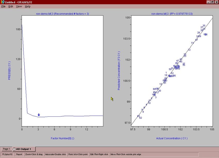
Bo

                      Precessional                         m=-
                      orbit around
                      applied
                      magnetic                       Spinning
                      field                          Nucleus

We can calculate the resonance frequencies for different applied field (Bo) strengths (in
Gauss):

                                                 1
                               Bo (T)                H Freq (MHz)
                                1.41                     60
                                2.35                     100
                                4.70                     200
                                7.05                     300
                                9.40                     400
                                11.75                    500

The field strength of a magnet is usually reported at the resonance frequency for a proton.
Therefore, for different nuclei with different gyromagnetic ratios, different frequencies
must be applied in order to achieve resonance.

                                   NMR Energies
The orientations that a nucleus’ magnetic moment can take against an external magnetic
are not of equal energy. Spin states which are oriented parallel to the external field are
lower in energy than in the absence of an external field. In contrast, spin states whose
orientations oppose the external field are higher in energy than in the absence of an
external field.

                                           -3-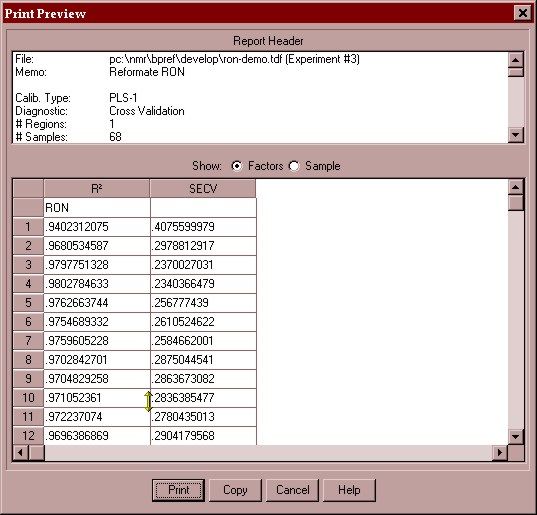
Bo

                                                                m = -1/2

 Relative
 Energy
                                                       I=1/2
                                             Bo
                                                                m = +1/2

                          Increasing Magnetic
                          Field Strength
Where an energy separation exists there is a possibility to induce a transition between the
various spin states. By irradiating the nucleus with electromagnetic radiation of the
correct energy (as determined by its frequency), a nucleus with a low energy orientation
can be induced to "transition" to an orientation with a higher energy. The absorption of
energy during this transition forms the basis of the NMR method. Other spectroscopic
methods, such as IR and UV/Visible, also rely on the absorption of energy during a
transition although the nature and energies of the transitions vary widely.

When discussing NMR you will find that spin state energy separations are often
characterized by the frequency required to induce a transition between the states. While
frequency is not a measure of energy, the simple relationship E=hυ (where E=energy,
h=Planks constant, and υ=frequency) makes this substitution understandable. The
statement "the transition (peak) shifted to higher frequencies" should be read as "the
energy separation increased".

                              Population Distribution

In a given sample of a specific NMR-active nucleus, the nuclei will be distributed
throughout the various spin states available. As the energy separation between these
states is comparatively small, energy from thermal collisions is sufficient to place many
nuclei into higher energy spin states. The number of nuclei in each spin state is described
by the Boltzmann distribution :

                                    Nupper /Nlower = e-γBo/kT

                                             -4-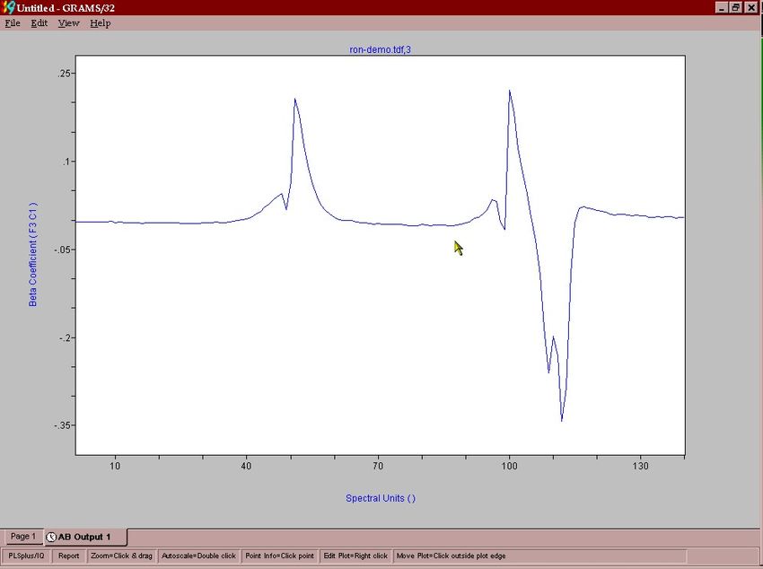
where the N values are the numbers of nuclei in the respective spin states, γ is the
magnetogyric ratio, h is Planck's constant, Bo is the external magnetic field strength, k is
the Boltzmann constant, and T is the temperature. For example, given a sample of 1H
nuclei in an external magnetic field of 1.41 Tesla, then the Population Ratio can be
written as:

Population Ratio =
    ((-2.67519x10⁸ rad.s-1.T-1*1.41T*6.626176x10-34 J.s)/(1.380662x10-23 J.K-1*K 293))
e                                                                                        = 0.9999382

Thus, at room temperature, the population ratio is 0.9999382. This plainly demonstrates
that the upper and lower energy spin states are almost equally populated with only a very
small excess in the lower energy state that represents spins aligned with the applied field.
The population difference is can be calculated as being only about 123 for every 4
million spins.

This nearly equal population distribution has a very important consequence. The amount
of signal intensity that one will observe in any spectroscopic method is proportional to
the population difference between the two energy levels involved. As an example, in
UV/Visible spectroscopy, the quantum energy levels have a large energy difference
which leads according to the Boltzmann distribution the population residin almost
exclusively in the lowest energy state. This means that UV/Visible spectroscopy is an
extremely sensitive technique that is typically used in analytical chemistry to deal with
very small amounts of sample. In NMR, the energy separation of the spin states is
comparatively very small to the point that, at room temperature, while NMR is very
informative from a chemistry stand-point, quantum mechanically it is considered to be an
insensitive technique. Thus NMR yields relatively weak signals that need to be signal
averaged for considerable periods to obtain spectra of adequate signal to noise. This also
leads to difficulties in using NMR for trace analysis. Typically NMr would not be
considered accurate below a quantitation of 0.05 wt% (500 ppm).

                   NMR Instrumentation – General Overview
There are two general types of NMR instrument; continuous wave and Fourier transform.
Early experiments were conducted with continuous wave (CW) instruments, and in 1970
the first Fourier transform (FT) instruments became available. This type now dominates
the market, and currently we know of no commercial CW instruments bing manufactured
at the present time.

Continuous Wave (CW) NMR instruments

Continuous wave NMR spectrometers are similar in principle to optical-scan
spectrometers. The sample is held in a strong magnetic field, and the frequency of the
source is slowly scanned (in some instruments, the source frequency is held constant, and

                                                      -5-
the magnet field is scanned). These systems are currently obsolete except for a few
wideline experiments that are performed in specialty solid-state NMR applications.

Fourier Transform (FT) NMR instruments

The magnitude of the energy changes involved in NMR spectroscopy are very small. This
means that, sensitivity can be a limitation when looking at very low concentrations. One
way to increase sensitivity would be to record many spectra, and then add them together.
As noise is random, it adds as the square root of the number of spectra recorded. For
example, if one hundred spectra of a compound were recorded and summed, then the
noise would increase by a factor of ten, but the signal would increase in magnitude by a
factor of one hundred - giving a large increase in sensitivity. However, if this is done
using a continuous wave instrument, the time needed to collect the spectra is very large
(one scan takes two to eight minutes).

In FT-NMR, all frequencies in a spectral width are irradiated simultaneously with a radio
frequency pulse. A single oscillator (transmitter) is used to generate a pulse of
electromagnetic radiation of frequency ωο but with the pulse truncated after only a
limited number of cycles (corresponding to a pulse duration τ), this pulse has
simultaneous rectangular and sinusoidal characteristics. It can be proven that the
frequencies contained within this pulse are within the range +/- 1/τ of the main
transmitter frequency ωο. For example a 5 μs pulse would generate a range of frequencies
of ωο ± 1/0.000005 Hz (i.e. ωο ± 200,000 Hz).

Following the pulse, the nuclei magnetic moments find themselves in a non-quilibium
condition having precesed away from their alignment with they applied magnetic field.
They begin a process called “relaxation”, by which they return to thermal equilibrium. A
time domain emission signal (called a free induction decay (FID)) is recorded by the
instrument as the nuclei magnetic moments relax back to equilibrium with the applied
magnetic field. A frequency domain spectrum that we are familiar with is then obtained
by Fourier transformation of the FID.

Effect of Applying a Radiofrequency Pulse

To understand the effect of the radio frequency pulse, we will consider the precessing
magnetic moments of the 1H nuclei in a sample sitting in an applied magnetic field:

                                           -6-
As discussed previously, there are more magnetic moments aligned with the field than
against it. This means that when all the opposing magnetic moments have cancelled each
other out, the net population difference will create a bulk magnetization vector (called
Mo) aligned along the direction of Bo. With this bulk magnetization vector concept the
magnetic behaviour of the spin system can be shown as follows:

Now we come to the “resonance” aspect of the NMR technique. One has now reduced the
magnetic moment system to a bulk magnetization vector. However, one must now take
into account the fact that the individual magnetization vectors for the nuclei are still
precessing around the applied field at the Larmor frequency (58 MHz in the case of the
DPS process NMR system). The trick in the NMR experiment is to find a way to perturb
these magnetic moments away from their alignment with the huge applied field by
utilizing the tiny field applied by a radio frequency pulse. This is a problem similar to

                                          -7-
what one would face when trying to push a friend off a carousel horse with your little
finger while the carousel rapidly spins past you at 58 million revolutions per second.
Timing would be essential! The way to do this is to jump on the carousel and poke your
friend in the eye causing them to fall off the horse. This “jumping on the carousel” can be
described as you joining your friends “rotating frame of reference”, in which the friend is
static with respect to the observer and can then be acted upon. In the NMR experiment
one applies radio frequency pulses at the Larmor frequency of the 1H nuclei being
observed in order to perturb the 1H magnetic moments with the magnetic component of
the applied RF electromagnetic radiation. In our diagrams below, a short RF pulse is
applied along the x' axis. The magnetic field of this radiation is given the symbol B1. In
the rotating frame of reference, B1 and M0 are stationary, and at right angles. The pulse
causes the bulk magnetization vector, M0 , to rotate clockwise about the x' axis. The
extent of the rotation is determined by the duration of the pulse. In many FT-NMR
experiments, the duration of the pulse is chosen so that the magnetization vector rotates
by 90°. In the case of the DPS process NMR system, the duration of the RF pulse is
chosen so that the magnetization vector moves through a 45o rotation.

The various reasons for performing 45o pulses rather than 90o pulses are related to the
relaxation rates of the spins. After each pulse one must wait for a “relaxation period”
which allows time for all the spins to equilibrate and line up with Bo again. By
performing a 45o pulse one can collect the NMR spectra at 3 times the rate that is
possible after performing a 90o pulse, while still acquiring 70% of the signal.

The detector is aligned along the y'-axis. If we return to a static frame of reference (i.e.
stop spinning the laboratory at the Larmor frequency) the net magnetic moment will be
spinning around the y-axis at the Larmor frequency. This motion of magnetic moments
constitutes a radio-frequency signal, which can be detected. When the pulse ends, the
nuclei relax and return to their equilibrium positions, and the signal decays. This
decaying signal contains the sum of the frequencies from all the target nuclei in the
sample. It is picked up in the coil as an oscillating voltage generated by the magnetic

                                           -8-
moments precessing/relaxing back to equilibrium. The signal cannot be recorded directly,
because the frequency is too high. It is mixed with a lower frequency signal to produce an
interferogram of low frequency. This interferogram is digitized, and is called the Free
Induction Decay, (FID). Fourier transformation of the FID yields a frequency domain
spectrum.

    FID - Time Domain Signal -Æ Fourier Transform -Æ Spectrum – Frequency Domain

             Chemical Shift and the NMR Spectrum
                    Sigma Electrons and Electronic Shielding

Electrons are negatively charged particles that surround nuclei within a molecule.We
know that moving charged particles will generate a magnetic field. For example, a stream
of moving electrons (electrical current) will generate a magnetic field around the
conducting wire that will cause the needle of a compass to align itself with the lines of
force generated by the magnetic field. Since electrons around nuclei in a molecule
generate their own magnetic field, the lines of force (magnetic moment) generated by this
magnetic field will run in the opposite direction as the lines of force generated by the
external magnetic field Bo. In fact, the electron's magnetic field runs anti-parallel to the
external magnetic field. When this happens, the electron-generated magnetic moment will
run in opposition to the magnetic moment of the external magnetic field. This has the
effect of reducing the net magnetic moment affecting the proton. This requires that the
external magnetic field be greater or higher in order to overcome this opposition so that
an NMR signal may be generated. This electronic magnetic field effect will cause protons
with different chemical environments to yield resonance frequencies perturbed from the
frequency defined by the applied external field Bo.

                                           -9-
The Larmor frequency can be re-written to include the electronic effect:

                                      ωo = γ(Bo – S)

where S represents the change in magnet field caused by the opposing electron magnetic
moment.

All electrons making up the sigma bonding around the nuclei will generate a magnetic
field that will be anti-parallel to the external magnetic field's lines of force. This causes
the NMR signal generation to occur at a higher external magnetic field setting. The NMR
signal is shifted upfield, and the protons are said to be electronically shielded. The word
shielded is used because the electronic magnetic moment actively shields the proton from
the external magnetic field such that the effect of the external field is not as great as it
could be if the proton was removed from an electronic environment.

Chemical Shift and the TMS Standard

We have now determined that chemically different protons have different electronic
environments. Differences in the electronic environments cause the protons to experience
slightly different applied magnetic fields owing to the shielding/deshielding effect of the
induced electronic magnetic fields. Over the years NMR spectra have been obtained on
every conceivable organic molecule in nature or synthesized in a lab. In order to
standardize the NMR scale it is necessary so set a 0 reference point to which all protons
can then be compared. The standard reference that was chosen is tetramethylsilane
(TMS). This compound has four CH3 methyl groups single bonded to a silicon atom. All
of the protons on the methyl groups are in the same electronic environment. Therefore
only one NMR signal will be generated. Furthermore, the electronegativity of the carbon
atoms is actually higher than the silicon atom to which they are bonded. This results in
the sigma electrons being shifted toward the carbon atoms in the methyl groups and
consequently, the protons will be heavily shielded causing the one signal to be generated
at a very high magnetic field strength setting. It is that signal that all other NMR signals
of a sample are referenced to. This association with the reference signal is called the
chemical shift. This shift is measured in parts per million (ppm). NMR signals occurring
near the TMS resonance are said to be in an upfield position while those shifted away by
deshielding are said to be downfield (see figure below)

Virtually all NMR signals will be further downfield from the TMS signal because of the
heavily shielded nature of the methyl protons in the TMS molecule. The proton NMR
chemical shift range is 0-12 ppm. The ppm scale is another form of standardization that
allows one to compare directly the 1H spectra obtained on NMR instruments with
different magnetic fields. After the samples have been referenced to the TMS resonance
at 0 ppm the actual NMR peak position in Hz is divided by the resonance frequency of
the spectrometer, which is in MHz. Thus, one is dividing Hz by MHz which is a part per
million (ppm). One ppm on a 58 MHz NMR instrument is actually 58 Hz from the
resonance position of TMS, while on a 300 MHz NMR instrument 1 ppm is 300 Hz from

                                           - 10 -
the TMS resonance position. With this standardization/normalization in place one can
always unequivocally say that all benzene protons resonate at 7.16 ppm no matter what
NMR instrument is being used in the analysis.
Downfield
Upfield
Aldehyde Aromatic
water Alpha-H Alkane
TMS
olefin oxygenate
10 5 0 ppm
In the DPS process NMR instrument we do not have an internal TMS standard available
to reference the on-line spectra. Instead, the NMR peaks in the spectrum itself are used to
reference the whole spectrum based on a well-established knowledge of the process
stream chemistry. The various aromatic, CH3 or CH2 groups in the spectrum can be peak-
picked and assigned to their known chemical shift values that have been logged in large
databases of NMR chemical shifts. Below is a diagram showing the chemical shifts of
some typical organic functional groups. The detailed chemical shift information related
specifically to petroleum chemistry is described more fully later on.
Proton NMR Chemical Shifts for Common Functional Groups
RNH2
R-CO-NH2
R-CH-OH
Alpha-H
Aromatic-H
H2O R-CH-O
RCHO R-CH-NR2
R-CH-Cl
R-COOH
Olefinic-H
Saturate-H
12 11 10 9 8 7 6 5 4 3 2 1 0 ppm
- 11 -• Electronegative groups are "deshielding" and tend to move NMR signals from
neighboring protons further "downfield" (to higher ppm values).
• Protons on oxygen or nitrogen have highly variable chemical shifts, which are
sensitive to concentration, solvent, temperature, etc.
• The -system of alkenes, aromatic compounds and carbonyls strongly deshield
attached protons and move them "downfield" to higher ppm values.
Relaxation
In most spectroscopic techniques, how the energy absorbed by the sample is released is
not a primary concern. In NMR, where the energy goes, and particularly how fast it "gets
there" are of prime importance. The NMR process is an absorption process. Nuclei in the
excited state must also be able to "relax" and return to the ground state. The timescale for
this relaxation is crucial to the NMR experiment. For example, relaxation of electrons to
the ground state in uv-visible spectroscopy is a very fast process, on the order of pico-
seconds. In NMR, the excited state of the nucleus can persist for minutes. Because the
transition energy between spin levels (discussed earlier) is so small, attaining equilibrium
occurs on a much longer timescale. The timescale for relaxation will dictate the how the
NMR experiment is executed and consequently, how successful the experiment is.
There are two processes that achieve this relaxation in NMR experiments: longitudinal
(spin-lattice) relaxation and transverse (spin-spin) relaxation.
In longitudinal relaxation energy is transferred to the molecular framework, the lattice,
and is lost as vibrational or translational energy. The half-life for this process is called the
spin-lattice relaxation time (T1). Dissipating the energy of NMR transitions (which are
tiny compared to the thermal energy of the sample) into the sample should not be a
problem, however T1 values are often long. The problem arises not in where to "send" the
excess energy, but the pathway along which the energy is released to the lattice.
Contributing factors to this type of relaxation are temperature, solution viscosity,
structure, and molecular size.
In transverse relaxation energy is transferred to a neighboring nucleus. The half-life for
this process is called the spin-spin relaxation time (T2). This process exchanges the spin
of nucleus A with the spin of nucleus B (A mI = -½ → +½ as B mI = +½ → -½. There is
no net change in spin for this process. Inhomogeneity of the magnetic field or the
presence of paramagnetic materials can be a large contributor to the value observed for
transverse relaxation.
The peak widths in an NMR spectrum are inversely proportional to the lifetime (due to
the Heisenberg uncertainty principle) and depend on both T1 and T2. For most organic
solutions, T1 and T2 are long enough to result in spectra with sharp lines. However, if
magnetic field homogeneity is poor or paramagnetic material (such as iron) is present the
NMR signals can be broadened to the extent that the signal is destroyed or unusable.
- 12 -Experimental Considerations Temperature, Tuning, Locking, Shimming The sample for an NMR experiment should not contain any particulate matter that may affect the field homogeneity within the sample. After the sample is stopped in the magnet it is necessary to tune the probe to get the most effective power transferred to the sample, and the most effective detection of the signal. Tuning the probe involves altering the complex impedance of the coil to minimize the reflected power. (This needs to be performed once during installation). After the probe is tuned it is necessary to "lock" the spectrometer on the external LiCl sample. Adjusting the Transmitter The next step is set the frequency of the pulses and to adjust the sweep (or spectral width). In general, spectrometer frequencies are specified using two parameters, a fixed number that depends on the magnetic field strength of the instrument and the observed nuclei, and a user adjustable offset that is added to the fixed number to give the frequency of the transmitted pulse. At the beginning the user defined offset is set to zero and a very large spectral width is used (e.g. 20 KHz). With such a wide window all of the resonance lines should fall in this frequency range. Since the time required for the 90o pulse is not yet known, the first spectrum is obtained using a short (6 μs) pulse. Once the position of the resonance peaks has been determined, the offset is moved to the middle of the spectrum and the spectral width is adjusted to be just large enough to span all of the resonance lines in the spectrum. The 90o pulse length is determined by observing the effect of the pulse length on the spectral intensity or on the FID signal intensity (RMS – root mean signal). The spectrometer frequency is set to be 300-500 Hz from the resonance frequency of the main resonances in the spectrum. The pulse length is set to 4 μs (e.g.
of the fields generated by the other shim coils. However, in practice there can be
considerable interaction and it is usually necessary to adjust several coils at the same
time. All magnets show drift, or a change in field strength, over time. These changes are
usually small enough that they can be compensated by adjusting the 1H transmitter
frequency to match the magnetic field / shim changes.

The Lock

Changes in the magnetic field strength are detected by measuring the resonance position
of Li7 in the external lock reference. Both the absorptive and dispersive components of
the Li7 resonance line are used in adjusting for field inhomogeneity. Based on the
absolute frequency of the Li7 resonance the transmitter frequency is adjusted to
compensate for changes in magnet, sample, or shim.

Generating the Pulse

The actual frequency of the RF pulse is generated by mixing two frequencies together.
The first, ωsyn is adjustable and is generated from the frequency synthesizer under
computer control. The second is an internal constant frequency called the intermediate
frequency, IF. After mixing of these two frequencies and amplification the signal is sent
to the probe. Since the same sample coil is used to both send the RF pulse and receive the
FID it is necessary to route the RF pulse to the coil and not to the pre-amplifier.
Otherwise the rather intense RF power may damage sensitive components in the pre-
amplifier. This routing is accomplished by grounding the circuit (using diodes) 1/4λ from
the junction point. Under these conditions the pre-amplifier side of the circuit appears as
an infinite resistance and most of the RF pulse goes to the sample coil.

Receiving the NMR Signal

The induced transverse magnetization is detected using the same coil that carried the RF
pulse to the sample. However, since the induced EMF in the coil is quite weak, the
grounded point in the pre-amplifier is not seen as a ground and the signal can pass the
1/4λ coil.

The frequency of the induced RF is quite high (e.g. 58 MHz). This is an extremely fast
rate (i.e. 58 MHz) and there are practical problems associated with operating analog to
digital converters at this frequency. Instead of trying to sample the magnetization at 58
MHz, the frequency of the signal is reduced to that in the rotating frame (audio range) by
mixing the signal first with ωsyn and then with the IF.

How to Obtain Quantitative NMR Spectra

The quantitative information of NMR is contained in the area under the various
resonances. A quantitative spectrum is simply a spectrum where you can trust the integral

                                          - 14 -
values and ratios. In other words, if the integral of resonance A is twice the height of the
integral of resonance B, you can say with certainty that resonance A is due to twice the
number of nuclei as resonance B. In the DPS process NMR instrument all spectra are
converted to integral values during the data processing step. We use integrals because it
is the area of the resonances that is proportional to the number nuclei. The height of a
broad line may be less than that of a sharp line, but its area may be greater. How do we
get accurate integrals? By ensuring that all resonances are equally excited, well digitized,
and properly relaxed.
o Equally excited : if the pulse power is not high enough, some resonances
far from the observe frequency may experience a reduced flip angle,
resulting in a smaller observed signal. Fix: ensure power levels are high
and that the spectrum is not offset to the edges of the spectrum.
o Well digitized : if the number of data points in the spectrum is too low,
there will not be enough points to accurately define each resonance,
resulting in inaccurate integrals (and peak heights). Fix: set ADC so that a
narrow spectral width is defined and the FID contains all signal and very
little noise – then zero fill to 8192 of 16384 points so that the spectral
resolution is improved for referencing and integral calculation.
o Properly relaxed : resonances that are not fully relaxed give a weaker
signal than fully relaxed resonances. The nuclei in your compound will not
all relax at the same rate, so if you pulse too rapidly the quickly relaxing
resonances will appear stronger than the slowly relaxing ones. To be sure
of obtaining accurate integrals, one must ensure that a 45o pulse is used
and that a relaxation delay is placed in the pulse sequence that is long
enough to prevent observable RMS reduction from the first pulse to the
second pulse. For small molecules in the gasoline range typical T1 values
are on the order of 8-30 seconds while larger molecules in the diesel range
are typically 4-20 seconds. The T1 of the longest relaxing molecule in the
mixture must be used. Thus, at 45o the recycle rate should be about 10 s
for gasoline range samples and 7 seconds for diesel range samples.
- 15 -Proton NMR of Refinery Streams
Table I shows the chemical shifts of the various functional groups found in petroleum
products.
Table I
Proton NMR Assignments for Functional Groups of Interest in Petroleum Chemistry
Peak
Position * Assignment (comments)
0.5-1.0 CH3 γ and further, some naphthenic CH and CH2 . Separation at 1.0 ppm is
generally not baseline resolved (ref a).
1.0-1.7 CH2 β and further. some β CH. Separation at 1.7 ppm is generally not base
resolved
1.7-1.9 Most CH, CH2, β hydroaromatic. This shoulder is one of the best available
ways to estimate hydroaromaticity (ref b).
1.9-2.1 α to olefinic. Only if a clear peak appears, associated with peaks at 4.5-6.0
ppm
2.1-2.4 CH3 α to aromatic carbons. Separation at 2.4 ppm is generally not base
resolved
2.4-3.5 CH, CH2 α to aromatic carbons
3.5-4.5 CH2 bridge (diphenylmethane)
4.5-6.0 Olefinic
6.0-7.2 Single ring aromatic
7.2-8.3 Diaromatic and most of tri- and tetraromatic. For differentiation of aromatic
ring multiplicity see Cookson and Smith(ref a) and Simmons (ref c).
8.3-8.9 Some tri- and tetraromatic rings
8.9-9.3 Some tetraromatic rings
* Referenced to TMS (tetramethylsilane) at 0 ppm (units = ppm)
ref a Cookson, D.J., Smith, B.E., in ‘Coal Science and Chemistry’ (Ed. A.
Volborth), Elsevier, Amsterdam,1987, pp31-60.
ref b Galya, L.G., Rudnick, L.R., Am. Chem. Soc. Div. Pet. Chem. Prepr., 1988, 33,
382.
ref c Simmons, W.W. (Ed.),’The Sadtler Handbook of Proton NMR Spectra’,
Sadtler Research, Inc., Philadelphia, PA, 1978.
On the following pages are several examples of 1H NMR spectra obtained on various
refinery streams. The hydrocarbon types that are observed are displayed on the spectrum.
Superimposed plots of the spectra show the typical variability that is observed as the
processes change over time. Typical modeled parameters and their reproducibilities are
also shown.
- 16 -Reformer Application
R
Benzene CH3
CH2
CH3
R
CH
R
H3C
10 8 6 4 2 0
PPM
Figure 1: Chemical Breakdown of 1H NMR Spectrum of Reformate
- 17 -Figure 2: Typical Variation of Processed NMR Data Observed in
Reformate Data Set
- 18 -Table II
Performance of Current On-Line Reformate PLS Models
Parameter R2 SECV # of Factors Range
RON 0.9895 0.23 O.N. 8 97-106 O.N.
Benzene 0.9850 0.23 Vol% 8 0.7-10.0 Vol%
MON 0.9852 0.19 O.N. 6 89 – 94 O.N.
RVP 0.9012 0.015 Bar 8 0.29 – 0.49 Bar
- 19 -Gasoline Application CH3
CH2
CH3
CH3
CH
H R
R H
R R
R H
H H R H
Oxygenate
8 7 6 5 4 3 2 1 PPM 0
Figure 3: H-Types Observed in a Gasoline 1 H NMR Spectrum
- 20 -1
0
8
6
4
2
0
20 40 60 80 100 120 140
Figure 4:Variability observed in Gasoline NMR spectra
- 21 -Table III
Summary of Cross Validation PLS Modeling for Gasolines
Validation Calibration
2
Parameter Variance SECV R Factors SEC R2
0.0020
Density 99.06 0.0024 g/ml 0.9984 5 g/ml 0.9991
Aromatics 98.79 0.77 Vol% 0.9994 5 0.64 Vol% 0.9996
Benzene 99.33 0.19 Vol% 0.9744 5 0.12 Vol% 0.9925
Olefins 99.73 1.41 Vol% 0.9938 6 1.15 Vol% 0.9967
MTBE 99.03 0.27 Vol% 0.9986 5 0.10 Vol% 0.9999
IBP 99.96 5.12 oC 0.9636 6 4.26 oC 0.9783
T10 99.49 4.22 oC 0.9905 6 3.59 oC 0.9942
T50 99.07 2.13 oC 0.9967 5 1.61 oC 0.9983
T90 99.81 2.15 oC 0.9982 7 1.41 oC 0.9989
FBP 99.57 4.11 oC 0.9896 6 3.28 oC 0.9946
RON 99.67 0.31 0.9968 8 0.22 0.9989
MON 99.79 0.35 0.9971 8 0.25 0.9989
RVP 99.87 0.026 bar 0.9956 9 0.014 bar 0.9990
Sulfur 99.69 61.7 ppm 0.9820 6 39.0 ppm 0.9949
- 22 -CH3
15
CH2
10
CH3
CH
CH3
5
0
H R
R H
R R
R H
H H R H
Figure 5: 1H NMR Spectral Variability Observed in Naphtha Cracker Feed Samples
d the Functional Chemistry Observed
- 23 -Table IV (Part 1)
Summary of Cross Validation PLS Modeling for Normal and Iso-Paraffins
Validation Calibration
Parameter Variance SECV R2 Factors SEC R2
Density 97.64 0.0031 0.9903 5 0.0021 0.9968
Normal-Paraffin 97.18 0.95 0.976 6 0.6 0.9929
n-C4 99.26 0.89 0.759 9 0.39 0.9725
n-c5 97.69 1.73 0.9525 6 1.05 0.9879
n-c6 99.19 1.25 0.9689 9 0.81 0.9809
n-c7 91.14 0.34 0.9595 3 0.27 0.9801
n-c8 99.36 0.36 0.9836 9 0.18 0.9978
n-c9 99.55 0.26 0.9843 10 0.15 0.9973
n-c10 98.95 0.14 0.9821 8 0.09 0.9947
Iso-Paraffin 98 1 0.9646 6 0.67 0.9888
I-c4 83.63 0.05 0.8084 3 0.04 0.9271
I-c5 99.69 1.01 0.9798 11 0.49 0.9975
I-c6 98.76 1.6 0.9557 7 1.07 0.9863
I-c7 99.66 0.89 0.9441 11 0.41 0.9939
I-c8 98.83 0.36 0.9893 7 0.22 0.9973
I-c9 97.34 0.3 0.9893 6 0.21 0.9964
I-c10 66.16 0.45 0.9705 1 0.41 0.9777
I-c11 80.69 0.03 0.9148 2 0.02 0.9479
I-c12 99.98 0.43 0.9205 13 0.06 0.9996
- 24 -Table IV (Part 2)
Summary of Cross Validation PLS Modeling for Olefins,
Naphthenes and Aromatics
Validation Calibration
2
Parameter Variance SECV R Factors SEC R2
Olefins 99.5 0.084 0.9779 11 0.061 0.9888
Naphthenes 99.21 0.81 0.9689 8 0.47 0.9934
Cyclopentane 99.32 0.11 0.9934 9 0.06 0.9986
Methyl-Cyclopentane 94.18 0.48 0.9678 3 0.41 0.9806
Cyclohexane 97.96 0.21 0.9924 6 0.14 0.9973
Methyl-Cyclohexane 99.2 0.43 0.9424 9 0.23 0.9904
c7-naphthenes 97.69 0.21 0.8151 4 0.16 0.9303
c8-naphthenes 99.72 0.32 0.9843 11 0.14 0.9984
c9-naphthenes 96.88 0.41 0.9845 5 0.27 0.995
c10-naphthenes 97.53 0.02 0.9249 5 0.01 0.9858
Aromatics 99.19 0.36 0.9956 9 0.17 0.9994
Benzene 99.43 0.06 0.9986 9 0.04 0.9996
Toluene 99.01 0.18 0.9721 8 0.11 0.9933
Xylenes 98.31 0.25 0.9833 7 0.15 0.9955
Ethyl-Benzene 99.38 0.07 0.9757 9 0.04 0.9948
C9-Aromatics 88.76 0.28 0.9704 2 0.25 0.9782
C10-Aromatics 87 0.06 0.9483 3 0.05 0.9736
- 25 -CH2
CH3
CH3
R R
R
H3C
10 8 6 4 2 0
ppm
Figure 6: Typical Variability Observed in
NMR Spectra of Blended Diesel Fuels
- 26 -Table V
Performance of On-Line NMR Gas Oil Blending Models
Parameter R2 SECV # of Factors Range
Cetane Index 0.9943 0.85 C.N. 7 21 to 56 C.N.
(D976)
Cetane Index 0.9925 0.91 C.N. 8 21 to 56 C.N.
(D4737)
Cloud Point 0.9746 5.6of 9 -87 to +45of
(D2500)
Pour Point 0.9737 5.7 of 9 -85 to +35 of
(D97)
T10 0.9332 10.4 of 9 312 to 496 of
(D86)
T50 0.9837 4.6 of 9 340 to 565 of
(D86)
T90 0.9842 5.2 of 8 400 to 662 of
(D86)
End Point 0.9733 9.8 of 8 445 to 694 of
(D86)
API Gravity 0.9940 0.60o 8 13 to 46o
(D4052)
Sulfur 0.9722 0.12 Wt% 8 0.01 to 1.92
(D2622) Wt%
Viscosity 0.9283 0.099 cSt 9 1.00-3.3 cSt
(D445)
- 27 -NMR Chemometric Modeling
Introduction
Chemometrics is the statistical processing of analytical chemistry data with various
numerical techniques in order to extract information. The technique utilized for the
Foxboro NMR product is partial least squares analysis which reduces the large amount of
spectral data obtained on a process stream and reduces the information into principal
components (factors) that describe the spectrum/measured parameter correlation in a data
reduced manner
Chemometric Modeling of Refinery Streams
The data processing routines that are commonly used with near-infrared spectroscopy in
analysis of refinery streams are being used to process the spectral data from the Foxboro
NMR instrument. A series of mathematical manipulations of the data are used with a
previously developed calibration model to predict the fuel content value of the property
of interest.
RAW DATA, X Æ Chemometrics: f(X) Æ MON, RON, Benzene, T90, Cetane etc.,
Mathematical Tools
Chemometric data analysis routines consist of proven mathematical tools from the
statistics and engineering literature. Tools range from baseline correction and smoothing
to multivariate analysis techniques such as partial least squares regression, PLS, principal
components regression, PCR, and neural networks. The detection of outliers and new
and different samples will be handled by hierarchical cluster analysis followed by
Mahalanobis distance testing of single-cluster subsets of the spectral data.
Why Use Chemometrics?
The complex relationship of fuel content to fuel property often requires a complex
solution. Consider the property of research octane number, or RON. The RON value of
a particular fuel depends in a complex way on the chemical composition of that fuel.
Aromatics tend to increase RON, while long and very short saturated chains tend to
decrease the RON value of a fuel. Each particular chemical species contributes uniquely
to the overall RON value of a fuel. Some types of molecules strongly influence
(negatively and positively) the RON number while others have a more modest influence.
Many fuel and distillate properties are a weighted function of the array of fuel
constituents. Chemometric techniques provide a means for extracting complex property
information from subtle variations in the fuel spectrum that arise from variations in the
array of chemical constituents present in the fuel sample.
- 28 -Long Term Modeling Approach
The ultimate goal in process modeling with chemometrics is to develop the “global”
multivariate calibration model. The global calibration model would be invariant through
time on one instrument and across different instruments. Little progress has been made on
the development of global models on near IR instruments over the past 10 years. The
global model would require that the calibration developed on one instrument be
transferred to other instruments and through time on a single instrument without a
significant loss of accuracy. This is a very challenging problem because of the
complexity of the model being transported.
Foxboro NMR recognizes that chemometric process models must be developed and
maintained. The strategy being implemented currently involves the updating of on-line
models with new data points currently not described in the calibration models. This step
is performed when a shift in the process is indicated by the appearance of outliers arising
from chemical variation of the process stream. The expected maintenance interval for a
given calibration is expected to decrease with time as the process variation is revealed
and incorporated into the model database.
Chemometric Regression Methods
Model Building Using Soft Modeling Methods
Modeling in the absence of a direct quantitative physical understanding of the relation
between the measurement variables(spectra) and the physical or chemical properties (e.g.
RON) to be determined requires a different approach when compared with models based
on well-defined physical systems. Take for example the property of Research Octane
Number, RON. RON is known to depend on the distribution of chain lengths and
fractional content of aliphatics, and on the distribution and fractional content of aromatic
species. Even if the exact impact (hard model) of each molecular type on the octane
number was quantitatively known, the accounting for the hundreds of chemical species
that make up a gasoline stream would require an exhaustive level of analysis to compute
the hard model for the fuel octane. Soft modeling with principal components makes use
of the statistical correlation of the data variation with the property variation in developing
a regression model.
Soft modeling was originally used in the behavioral sciences in an attempt to extract
expected behaviors from complex multivariable observations. Modeling in the behavioral
sciences is complicated by the selection of observations that are related to the behaviors
of interest. Fortunately, the intuitive link between spectroscopic measurements and
physical or chemical properties is much easier to establish. For example, it is known that
7-9 carbon straight chain aliphatics increase octane and that aromatics also increase
octane. Aliphatics with a high degree of branching also increase the octane value of a
fuel. Spectroscopy provides information on the chemical structure variation contained in
- 29 -the fuel mixture. Therefore chemical intuition can be used to support the development of
regression models that relate the spectral responses to the octane number of fuels.
Multivariate Regression Models
Many engineers and scientists are familiar with the concept of linear regression. In linear
regression a single independent variable, y, is regressed against a single dependent
variable, x. The form of the regression model is:
y = bx + int (1)
Equation 1 requires 2 pairs of (x,y) data (2 points to define a line) since there are two
unknowns to be solved, b and int. This theme of the number of data samples meeting or
exceeding the number of unknowns to be determined is a very important concept that
must be met in order to determine meaningful regression solutions. The solution to
equation 1 is obtained by regressing known values of y against the corresponding known
values of x. The unknown free parameters to be solved are the slope b, and the intercept,
int.
In spectrometry, a line is used to develop a calibration between concentration, c, and
absorbance, x, according to beer’s law.
c = bx + int (2)
It is possible to extend the regression relation to multiple concentration and absorbance
variables. A vector is denoted by using a boldface lower case character, and a matrix is
denoted by a boldface upper case character. The concentration vector includes the
concentration of n sample constituents, a 1 by n dimensional vector.
c = xB + int (3)
Note that equation 3 has a 1 by n vector of concentrations(1 sample with n constituents),
a 1 by m vector of spectral measurements, x, and an n by m matrix of regression
coefficients(slopes) to be solved: (1 by m)(m by n) gives a 1 by n dimensional
concentration vector.
If c and x are mean-centered, the intercept term is zero.
c = xB (4)
Equation 4 is the form of a multivariate predictive model that is used in the estimation of
the property or concentration values of a sample with measured spectral response x. The
predictive model is defined by B, the matrix of regression coefficients. A multivariate
calibration model must be calculated to obtain B. In the calibration sequence, multiple
- 30 -samples are required to ensure a unique solution of B and the variables in the expression
are all matrices.
C = XB (5)
The matrix of unknown free parameters, B, is solved by a multivariable matrix regression
B = (XTX) –1 XTC (6)
–1
Where the superscript T is used to denote the matrix transpose, and the superscript is
used to denote the matrix inverse.
It is important to note that the matrix B, is dimensioned as m by n, the number of number
of wavelengths, m, by the number of constituents, n. Equations 5-6 describe the multiple
linear regression model, MLR. If it is desired to increase the available spectral
information in the model, more spectral wavelengths are included. One of the problems
with MLR is that the size of the B matrix of unknowns grows rapidly as more spectral
wavelengths are included in the regression model. This means that the number of
calibration samples with known property/concentration values must also grow rapidly as
more wavelengths are included in the model. The failure to use an adequate number of
calibration samples can result if a catastrophic failure of the model in the prediction
mode. Another problem with MLR is that, for spectral data that exhibit subtle variations
with the typical process variation, the matrix inverse step is poorly conditioned. A poorly
conditioned system will lead to large errors in the computation of the regression
coefficient matrix B, and resulting poor prediction accuracy. A poorly conditioned
calibration matrix will lead to models that will be extremely unreliable in predicting on
samples with spectra that are dissimilar to those spectra contained in the calibration set
data. Dissimilar spectra are likely to be encountered with a changeover in blending
feedstock or formulation (winter/summer) changes in the product.
Latent Variable Based Soft Models
The aforementioned difficulties with MLR are addressed with latent variable regression
methods. A latent variable is defined as a variable that is not directly observable, but is
related to the observable variable. The observable variables, usually spectral intensities or
absorbances, are used to generate latent variables. A latent variable, t, is the result of a
weighted linear combination of the observable variable vector elements, x.
t = p1x1 + p2x2 + p3x3 + p4x4 + p5x5 + … pmxm (7)
Thus, information from m wavelength measurements can be compressed into 1 latent
variable. The weighting coefficients, pi , in equation 7 are called the loadings, and p is the
loadings vector. In practice, more than one score variable is required to capture the
relevant chemical variance of complex samples. The spectral matrix is eigen-decomposed
into a number of scores and loadings vectors and some analysis is required to determine
- 31 -the number of that are needed to capture the chemical variation inherent in the chemical
system. The number of relevant scores kept is typically between 5 and 10 when
calibrating on petroleum distillate streams. Most of the methods of eigen-decomposing
spectral data yield orthogonal or nearly orthogonal sets of scores. Orthogonalization of
the spectral data addresses the problem of inverting a poorly conditioned spectral
calibration matrix, and the relatively small number of score terms used can dramatically
reduce the number of free parameters to be solved. This means that fewer samples are
required to over-determine the calibration model. For example, the use of 500 wavelength
measurements to determine 5 constituents would require 500*5 or 2500 unique sample
spectra. If 10 scores were used in place of the raw spectra, 10*5 or 50 samples would
represent the number of samples to exactly determine the chemical system. Experience
has determined that reliable models should be over-determined by 2-3 times, therefore
100-150 samples (as opposed to 50) would be a good starting point to model a system
with 10 significant scores.
Building of PLS/PCR Models
The two most common latent variable modeling methods are principal components
regression, PCR, and partial least squares, PLS. They are essentially equivalent in
modeling accuracy with the following exceptions:
1) PLS may have an advantage in modeling systems that contain uncorrected baseline
variation or pink noise.
2) PCR may have an advantage in systems that contain more than 6 significant score
variables.
The basic difference between the two is that the PLS algorithm uses information in the
independent variable matrix of properties/concentrations to direct the decomposition of
the spectral matrix into loadings vectors and scores while the PCR algorithm decomposes
the spectral matrix sequentially in the direction of maximum spectral variance, subtracts
the contribution on the maximal axis of variance from the spectral matrix, and then
repeats the process along the maximum direction of variance in the residual spectral
matrix that is orthogonal to the previously determined loadings vectors. This process is
continued until the variance in the spectral matrix is completely eigen-decomposed.
The following discussion on process modeling specifics will focus on the use of PCR,
though the choice of method actually used in process modeling will be determined by
prediction accuracy.
Model Development Environment
Proprietary algorithms used in generation of calibration models, calibration transfer and
spectrum pre-processing have and will be developed in the MATLAB programming
- 32 -environment. The PLS and PCR modeling program used to develop the process
chemometric models is Galactic Grams PLS/IQ.
Principal Components Regression, PCR
Consider fuel spectra that are arranged in rows of a matrix of spectral data, X, with
measured property values for each fuel sample represented in the property matrix Y. The
development of the PCR calibration model is performed as follows:
First, the row spectral matrix X is decomposed into an orthogonal basis set of scores,
T(projections), and loadings vectors contained in the matrix P as in Equation 1. The set
of loadings vectors make up the basis for the new coordinate system. The new coordinate
system is used to define the NMR spectrum in terms of new variables that are fewer in
number than the frequency range variables that makes up the original NMR frequency
coordinate system. The redefining of coordinates is analogous to the conversion from
rectangular to polar coordinates, though coordinate changes in a PCR decomposition only
require linear transformations. The values of the spectral intensities in the new coordinate
system are the spectral scores, T.
X = TPT (8)
Selection of Principal Components
The number of coordinate (loadings) axes chosen to represent the spectral data (number
of principal component scores) is a critical decision that will be made using a variety of
criteria. The inclusion of too many scores leads to good fits of the model but sub-optimal
prediction due to the inclusion of excess noise in the calibration model. The inclusion of
too many scores leads to a model with excessive bias or systematic error in fitting and
prediction. There are a number of methods (like PRESS, indicator function, f-test) that
have been used to determine the optimal number of scores, but since some of these
methods are statistically based and include statistical assumptions of data homogeneity,
the most reliable method of determining the optimal number of scores is by expert
inspection of the data structure. A careful study of the spectral calibration matrix is
conducted and the residual errors fitted with the addition of each principal component are
examined. Unusually large projections of a single sample on a single loadings axis can be
indicative of one unusual sample dominating the score. In this case the score will be
excluded from the model. In process modeling, the removal of one extra score component
than the apparent optimal number, is often used to define models as it is easier to
compensate for model bias than model noise.
Once the spectral scores of the calibration set spectra are obtained, they are then used
along with the known matrix of property values to solve for the matrix of regression
coefficients, B, which define the PCR calibration model.
B = (TTT) –1 TTY (9)
- 33 -The calibration model is defined by the loadings matrix, P, and by the matrix of
regression coefficients, B. Once the model is defined, the forward prediction step can be
used in the evaluation of fuel properties as follows:
First, obtain the vector of scores, ti , for the ith fuel sample by projecting the sample onto
the basis set or loadings matrix of the calibration model, P.
ti = xiP (10)
The prediction of the fuel properties, c, for the ith sample are obtained by right hand
matrix multiplication of the scores vector by the matrix of regression coefficients as in
Equation 4.
c i = t iB (11)
Sampling Requirements
There are well-defined statistically designed sampling guidelines for modeling with
multivariable systems. A statistical design of the simplest type, a two-level design,
requires two samples for a line (a univariate system: 1 independent variable), four for a
plane (2 independent variables), eight for a cube (three variables) and so on. The formula
for a statistical design of this type is 2n samples, where n is the number of variables in the
system. Samples are strategically chosen in a high-low format in each variable with all
combinations of high-low in each dimension accounted for. This design provides for
interpolation of all samples that fall inside the (hyper)volume bounded by the calibration
set measurements. Failure to use a statistical calibration design means that extrapolation
of the calibration model along one of the loadings axes is likely to occur in the prediction
mode.
Statistically designed calibrations models are not practical in many process applications
because the extremes of the process are undesirable and therefore extreme samples are
typically unavailable. This fact necessitates an alternate strategy for building process
calibration models:
1) An initial group of samples is selected containing as much of the process
variation as possible. The model is built on these samples and the future
prediction samples are evaluated in the prediction mode.
2) If a prediction sample appears to represent a variation that is not present in the
calibration set, the sample is captured, evaluated with the reference method
(e.g. octane engine) and the model is rebuilt with the inclusion of that sample
in the calibration set.
- 34 -Approximately 50-75 fuel samples, each with lab determined property values, are needed
to initially define a model containing 6-8 significant score components.
Model Adjustments
An adjustment of the model is dictated by the (automated flag) detection of process fuel
spectra that are dissimilar to the existing fuel spectra in the model database. The
differences could be due to considerable changes in chemical composition of fuels,
malfunction of sampling hardware or spectrometer The detection of an unusual sample
triggers a lab test, a graphical evaluation of the sample spectrum and, if necessary, a
recalculation of the chemometric regression model including the new sample(s). These
situations can arise from, process changes, unusual process disruptions/maintenance,
changes in regulations concerning fuel content, or from absence of some (seasonal)
variants of the fuel composition. In the case of regulation changes, some of the older
fuels will be excluded from the model database so that the model reflects current
blending targets. Model adjustments are commonly accepted among refiners that use
spectrometry as a part of a unified process control strategy. It is felt, however, that model
adjustments for NMR based models will be much fewer in number once a wide range of
process conditions have been included in the model.
The “outlier” sample in question would be linked to a cluster in the calibration set and a
Mahalanobis distance (a covariance matrix, C, scaled Euclidean distance) would be used
to determine if the sample belongs to the identified cluster.
D = [(x-u)C–1 (x-u)T]1/2 (12)
The Mahalanobis distance of normally distributed spectral data is known to follow the χ2
(chi-squared) distribution, permitting a test against a 95% confidence limit, assuming that
the data are homogeneous and normally distributed. This test also assumes that enough
data have been collected to obtain an accurate estimate of the sample population co-
variance matrix, C. In the real world of refinery measurements, the data are clustered
according to stream and the assumption of homogeneity fails. The normality of the data
may also be in doubt, but the Mahalanobis distance is somewhat tolerant of modest
deviations from normality.
To prevent the use of the Mahalanobis distance on a heterogeneous (multiple cluster) data
set, the calibration set data will be partitioned into individual cluster groups and a class
covariance matrix will be calculated for each cluster. This step will be performed using
hierarchical clustering to establish the number of clusters, and then self-organizing
clustering to assign cluster membership. The Mahalanobis distance of the sample will be
calculated for each cluster and the sample will be evaluated with the χ2 test statistic at the
95 % confidence level to determine is sample belongs to an existing cluster. If it is
determined that the sample does not belong to an existing cluster and it is determined that
there was no hardware malfunction, the model would be rebuilt with inclusion of the
outlier sample in the calibration data set.
- 35 -You can also read