A Comparative Analysis on Probability of Volatility Clusters on Cryptocurrencies, and FOREX Currencies
←
→
Page content transcription
If your browser does not render page correctly, please read the page content below
Journal of
               Risk and Financial
               Management

Article
A Comparative Analysis on Probability of Volatility Clusters on
Cryptocurrencies, and FOREX Currencies
Usha Rekha Chinthapalli

                                          Independent Researcher, H. No: 5-7-12, Housing Board Colony, Pakabanda Bazar, Khammam 507001, India;
                                          usha.bandu@gmail.com

                                          Abstract: In recent years, the attention of investors, practitioners and academics has grown in cryp-
                                          tocurrency. Initially, the cryptocurrency was designed as a viable digital currency implementation,
                                          and subsequently, numerous derivatives were produced in a range of sectors, including nonmonetary
                                          activities, financial transactions, and even capital management. The high volatility of exchange rates
                                          is one of the main features of cryptocurrencies. The article presents an interesting way to estimate the
                                          probability of cryptocurrency volatility clusters. In this regard, the paper explores exponential hybrid
                                          methodologies GARCH (or EGARCH) and through its portrayal as a financial asset, ANN models
                                          will provide analytical insight into bitcoin. Meanwhile, more scalable modelling is needed to fit
                                          financial variable characteristics such as ANN models because of the dynamic, nonlinear association
                                          structure between financial variables. For financial forecasting, BP is contained in the most popular
                                          methods of neural network training. The backpropagation method is employed to train the two mod-
                                els to determine which one performs the best in terms of predicting. This architecture consists of one

                                          hidden layer and one input layer with N neurons. Recent theoretical work on crypto-asset return
Citation: Chinthapalli, Usha Rekha.
                                          behavior and risk management is supported by this research. In comparison with other traditional
2021. A Comparative Analysis on
                                          asset classes, these results give appropriate data on the behavior, allowing them to adopt the suitable
Probability of Volatility Clusters on
                                          investment decision. The study conclusions are based on a comparison between the dynamic features
Cryptocurrencies, and FOREX
                                          of cryptocurrencies and FOREX Currency’s traditional mass financial asset. Thus, the result illustrates
Currencies. Journal of Risk and
Financial Management 14: 308.             how well the probability clusters show the impact on cryptocurrency and currencies. This research
https://doi.org/10.3390/                  covers the sample period between August 2017 and August 2020, as cryptocurrency became popular
jrfm14070308                              around that period. The following methodology was implemented and simulated using Eviews
                                          and SPSS software. The performance evaluation of the cryptocurrencies is compared with FOREX
Academic Editors: Jong-Min Kim and        currencies for better comparative study respectively.
Shigeyuki Hamori
                                          Keywords: cryptocurrency; FOREX currencies; volatility clusters; volatility persistence; cryptocurrency
Received: 26 April 2021                   market
Accepted: 24 June 2021
Published: 6 July 2021

Publisher’s Note: MDPI stays neutral      1. Introduction
with regard to jurisdictional claims in
                                               Volatility is commonly employed for estimating the distribution of returns on a given
published maps and institutional affil-
                                          financial asset to assess financial market instability. The simulation and estimation of
iations.
                                          volatility, therefore, play a significant role in the management and pricing of derivatives
                                          (Kočenda and Moravcová 2019). Most of the time, own-currency volatilities explain
                                          substantial share of exchange rates movements. While volatility is not explicitly observed,
                                          several volatility measures are suggested. The dynamic of this “observed” volatility
Copyright: © 2021 by the author.
                                          mechanism was then built to model and predict (Ramos-Pérez et al. 2019). For decades,
Licensee MDPI, Basel, Switzerland.
                                          different models of volatility were tested. Numerous models imitate major swings in
This article is an open access article
                                          cryptocurrencies and currencies; at the same time, smaller models are more prone to follow
distributed under the terms and
                                          modest price fluctuations. The pattern of significant market swings in the financial asset is
conditions of the Creative Commons
                                          known as volatility clustering (Pongsena et al. 2018), resulting in these price shifts being
Attribution (CC BY) license (https://
                                          permanent. In modelling volatility clusters, financial literature is relevant as the market
creativecommons.org/licenses/by/
4.0/).
                                          conditions are considered a key market risk predictor.

J. Risk Financial Manag. 2021, 14, 308. https://doi.org/10.3390/jrfm14070308                                 https://www.mdpi.com/journal/jrfm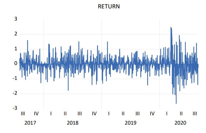
J. Risk Financial Manag. 2021, 14, 308                                                                                             2 of 23

                                              The amount of trade contains some commodities, including derivatives, making
                                         volatility their most important pricing factor, which increases over time. In the past several
                                         decades, the FOREX markets and their operations have changed dramatically. The days
                                         have passed when foreign exchange transactions are utilized in central banks, investment,
                                         and business. The presence of multinational businesses, private investors, speculators,
                                         hedge funds, individual investors, and arbitration companies in foreign exchange trans-
                                         actions has affected global and economic integration. From a conventional limited hour,
                                         the foreign exchange market has shifted operational structure to a 24-h electronic-based,
                                         market-oriented mechanism. With an estimated daily transaction of 3.2 trillion USD, this
                                         market is already considered the world’s largest financial market. The aforementioned
                                         dynamics have endowed the FOREX market with a particular characteristic known as
                                         “volatility” (Ho et al. 2017). In controlling the exchange rate flutter and alleviating negative
                                         consequences of cross-market disruptions, i.e., currency markets and through commodity
                                         that could harm individuals and companies alike, especially for corporations and poli-
                                         cymakers, modelling volatility exchanges across commodity and currency markets are
                                         especially relevant. Emerging markets are more susceptible to global shocks and lack an
                                         active derivatives market where market participants may hedge against currency risks
                                         are more concerned with this issue (Rognone et al. 2020). Different studies have added
                                         to the commodity currency nexus literature from several perspectives and have shown
                                         broad data from mature and developing economies with relevant impact on practitioners
                                         and policymakers. The variance is among the most significant parameters in several ran-
                                         dom processes for process recognition. In recent decades the association between sudden
                                         instability and crises has become stronger (Asai et al. 2020).
                                              The comprehensive behavior of the financial series shows that the major fluctua-
                                         tions seem more clustered than minor ones, and big losses, for example, tend to lump
                                         more than major gains together (Catania and Proietti 2020). Appropriate calibration of
                                         uncertainty and market risk are among the most daunting problems facing businesses
                                         that have to handle their assets’ inherent vulnerability or financial actions, for example,
                                         pension funds, banks, or insurers. During the 2007–2008 financial crisis, when market risk
                                         and volatility forecasting algorithms failed, this became even more apparent. Some pos-
                                         sible hedging possibilities are discovered based on the computed correlations between
                                         the bitcoin market and other assets (Tan et al. 2019). At the same time, the time series
                                         conditional variance are calculated according to different model specifications of ARCH.
                                         When the market is in chaos, the daily price restriction mechanism acts as a circuit breaker.
                                         However, when it comes to the link between PLH (Price Limit Hits) and market volatility
                                         (Reus et al. 2020). The supporters claim that price limits are efficient for minimizing price
                                         volatility, as, after the limits hits, the system effectively interrupts order flow. The op-
                                         ponents maintain, however, that the PLH serve as a magnet for enticing more traders,
                                         resulting in greater price volatility.
                                              In addition to returning causalities, the causal influence from currencies to commodi-
                                         ties occurs in volatility cases, often suggesting major transmissions from currencies to
                                         danger. It became apparent that the distributed ledger might be used to reduce investment
                                         risk by increasing public understanding about Bitcoin, which is crucial for the exchange
                                         market (Altan et al. 2019). Many contemporary theories focus on conditional variance or
                                         volatility, which measures the degree of unexpected return shifts and may thus be thought
                                         of as a random variable in a stochastic process (Kim et al. 2019). The class of models,
                                         which have been widely analyzed in literature as risk models of several financial time
                                         series, is based on a univariate GARCH model. The accuracy of the volatility projections
                                         increases by giving kurtosis and skewness for longer maturity solutions (Belasen and
                                         Demirer 2019). Compared with the electronic central money generated by the bank sys-
                                         tems or central banks (Samirkaş 2020), cryptocurrencies are decentralized and distributed.
                                         Blockchain Technology exercises control of this distributed system. Blockchain Technology
                                         (Dritsaki 2019) launches modern cryptocurrencies and verifies crypto puzzles decod-
                                         ing transactions.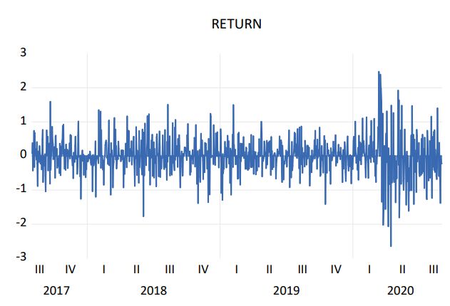
J. Risk Financial Manag. 2021, 14, 308                                                                                            3 of 23

                                              In many financial models, the main underlying assumption is the consistency of
                                         the model, but this assumption is generally not fulfilled because financial returns could
                                         include systemic breaks due to regulatory, operational, or technical changes and economic
                                         policy changes or significant macroeconomic shocks (Liu et al. 2020). Due to the variety
                                         of dynamics over time, the existence of disturbances influences the efficiency of forecasts.
                                         A method based on the modification of the estimate window for the prediction model
                                         can be employed to fix possible structural splits. This research explores the clustering
                                         of uncertainty in various properties, i.e., cryptocurrencies, and FOREX currencies. The
                                         financial assets are known to be cryptocurrencies, FOREX reserves, and currencies. This
                                         comparative study of the two financial properties would be demonstrated with the GARCH
                                         and the ANN models. Five days in advance are also expected for volatility, with value
                                         relative to real values. By measuring different indicators on the instability of financial
                                         markets, the findings of this analysis validate the key provisions of the principle of early
                                         detection of crisis.
                                              This article has six sections; Section 1 dealt with introduction. Section 2 examines the
                                         review literature, and Section 3 outlines the statement of problems. Section 4 reflects on
                                         research methodology; Section 5 continues with results and discussion. The study of this
                                         research paper is concluded in Section 6.

                                         2. Literature Review
                                               The volatility of an asset, which determines the distribution of this variable’s outcomes,
                                         plays a vital role in a variety of financial applications. Its key use is to quantify the
                                         consumer risk-benefit. Volatility is also an important price parameter for financial goods.
                                         Both modern models of option pricing are based on a price valuation volatility parameter.
                                         Volatility is also used in applications for risk control and fund management in general.
                                         In addition to the present valuation of the fluctuations of the controlled assets, financial
                                         institutions need to be able to predict their potential values. For institutions engaged in
                                         options trading and portfolio management, volatility forecasting is particularly relevant.
                                               (Koosakul and Shim 2021) published a document analyzing the precision of some of
                                         the most shared volatility projections: historical models for volatility (including exponen-
                                         tially weighted motion average), the implicit models for volatility, and autoregressive and
                                         heteroskedastic models. The model’s estimation accuracy is checked for the S&P 500 price
                                         index, demonstrating the benefits and drawbacks of each model.
                                               (Wen and Wang 2020) examined total and directional volatility connectedness in global
                                         foreign exchange (FX) markets. The variance decomposition approach was used to build
                                         a high-dimensional volatility network using 65 major currencies; the author includes the
                                         volatility overflow rate and LASSo-VAR methods. The empirical data show that the U.S.
                                         dollar and the Euro are large transmitters of volatility, whereas others, such as the Japanese
                                         yen and the British pound, are net receivers of volatility. In the volatility connectivity
                                         network, currencies are often categorized based on geoFigureical distributions. Total
                                         volatility links react dynamically to changes and growth in global economic fundamentals
                                         during moments of crisis.
                                               (Maciel and Ballini 2017) introduced the range-based modelling of volatility to define
                                         and estimate return-based models of conditional volatility. It involves the inclusion of
                                         the range calculation defined as the distance among the maximum and the leased asset’s
                                         prices within a time frame as an exogenous variable in General Autoregressive Conditional
                                         Heteroscedasticity (GARCH) models. It assesses whether range offers more knowledge
                                         about the intraday volatility mechanism and enhances estimation in comparison with
                                         GARCH-type approaches.
                                               (Cho et al. 2020) proposed an effective worldwide currency portfolio that may consid-
                                         erably reduce the risk of an exogenous global equity portfolio. The Japanese yen, Swiss
                                         franc, the U.S. dollar, and Euro move in a way that is contrary to the international equities
                                         market. The relevance of safe currencies to optimum currency portfolios has risen in terms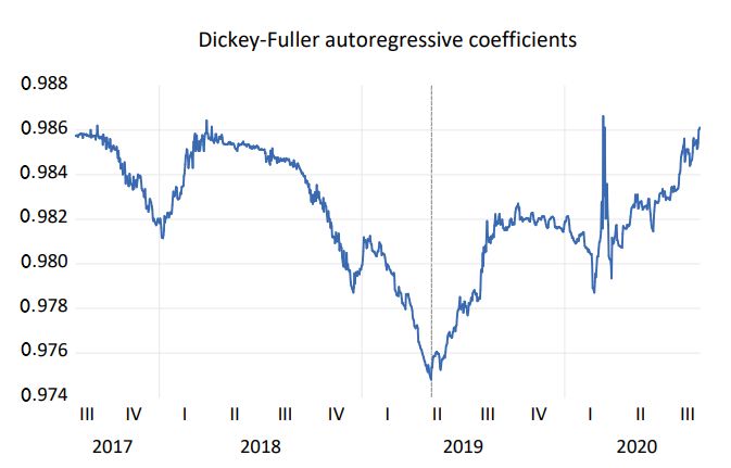
J. Risk Financial Manag. 2021, 14, 308                                                                                             4 of 23

                                         of foreign currency volatility in the U.S. stock market, and the impact of foreign exchange
                                         market volatility is greater than the impact on U.S. stock volatility.
                                               (Su 2021) investigated the volatility spillover magnitudes and drivers in the FX market
                                         using the realized volatility measurements and the HAR. This verifies both the impact
                                         on meteor showers (e.g., interregional spillovers of volatility) and on heatwaves (e.g.,
                                         spillovers of intraregional volatility). Market state variables contribute to more than half of
                                         the explanatory power in predicting conditional volatility persistence. With this model, that
                                         calibrates volatility persistence and spillovers conditionally on market states performing
                                         statistically and economically better. (Katusiime 2019) examines the influence of financial
                                         sector stability on commodity price volatility spillovers. Volatility spillover is investigated
                                         using the proposed techniques. Overall, the results of both the GVAR and MGARCH
                                         techniques indicate low levels of volatility spillover and market interconnectedness except
                                         during crisis periods, at which point cross-market volatility spillovers and market inter-
                                         connectedness sharply and markedly increased. (Arellano and Rodriguez 2020) suggested
                                         the weekly data for stock and FOREX market returns, a set of MS-GARCH models are
                                         estimated for a group of high-income (HI) countries and emerging market economies
                                         (EMEs) using algorithms allowing for a variety of conditional variance and distribution
                                         specifications. In the Latam FOREX market, estimates of the heavy-tailed parameter are
                                         lower than in the HI FOREX market and some other stock markets. In the FOREX markets,
                                         when leverage effects may not present in single-state models such as MS-GARCH, however,
                                         this does not happen.
                                               (Salisu et al. 2018) integrated the volatility spillovers and return in global FX markets
                                         using the world’s six greatest traded currency pairs, specifically the Euro, Swiss, gopher,
                                         loonie, Aussie, and cable. The research also conducted a rolling analysis of samples to
                                         record secular and cyclical moves in world FX markets. This revealed that the largest traded
                                         currency pairings are interdependent in accordance with spillover indices. In addition,
                                         return spillovers exhibit mild trends and bursts while volatility spillovers exhibit significant
                                         bursts but no trends. Further, identify crisis episodes that seem to have influenced the
                                         recorded fluctuations in returns and volatilities of global FX markets. (Nikolova et al. 2020)
                                         introduced a novel technique for estimating the likelihood of volatility classes with specific
                                         attention given to cryptocurrencies. To this end, the researcher used the FD4 method to
                                         compute the Hurst exponent of the volatility sequence. A particular criterion was defined
                                         to compute whether there are fixed-size volatility clusters. As a commonly used metric to
                                         calculate long-term store stock markets, the self-similarity index was consolidated. The
                                         report on the development of the S&P 500 self-similarity index, which was also introduced
                                         by (Segovia et al. 2019). It was exposed that the more often volatility changes are made
                                         (rather than normally falling into the index), the larger the exponent for self-similarity is
                                         and the more probable it is that clusters of volatility will form.
                                               (Swapna et al. 2015) proposed modified cluster data sets for teaching–learning based
                                         optimization (MTLBO) without prior knowledge of the number of clusters. The proposed
                                         technique determines effectively how many clusters or partitions are used while the
                                         program is executing. The suggested procedure is confined to partial clusters inspired
                                         by the algorithm of the K-means. The findings achieved by MTLBO are compared with
                                         the traditional method of TLBO and conventional differential evolution (DE). The results
                                         reveal that, in terms of function evaluations and cluster validity measurements, MTLBO
                                         offers greater accuracy than the two others.
                                               A worldwide model to forecast currency crises was offered by (Alaminos et al.
                                         2019). It utilizes a sample of 162 nations that allows the geoFigureical variability of the
                                         warning signs to be taken into consideration. The approach utilized was deep neural
                                         decisions (DNDTs), a methodology based on decision-making trees carried out by deep
                                         neural learning networks, and it is frequently employed in prediction compared to other
                                         techniques. This approach has considerable potential to bring macroeconomic policy into
                                         line with the risks arising out of currency declines to maintain global financial stability.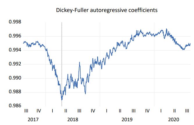
J. Risk Financial Manag. 2021, 14, 308                                                                                              5 of 23

                                         3. Statement of Problem
                                               In terms of portfolio management, the configurations of the Volatility Clustering
                                         Effect play key roles in the fields of portfolio management, notably asset allocation. The
                                         financial literature is interested in modelling clusters of volatility, as the latter is seen
                                         as a major market risk signal. The volume of trade in some assets such as derivatives
                                         is increasing over time, and volatility is becoming their main value. Financial volatility
                                         submits two fascinating empirical regularities that apply to various assets, markets, and
                                         time scales: it is fat-tailed (more precisely power-law distributed) and it tends to be
                                         clustered in time. In this article, the cryptocurrencies are positioned by comparing their
                                         dynamic features with one traditional and widely accepted financial asset of FOREX
                                         currencies. The investigator’s initial analysis is based on the daily starting and closing
                                         price for about four years based on five components: volatility, centrality, cluster structure,
                                         robustness and risk of cryptocurrencies and FOREX currencies. Based on the result obtained
                                         from the analysis, a comparative analysis of the two different financial assets has to be
                                         illustrated. Volatility is projected 5 days ahead, and values are compared to the real value
                                         in order to determine the performance of models for the prediction of volatility.

                                         4. Research Proposed Methodology
                                               The study’s key aims are to compare the prediction effects on volatility between the
                                         hybrid GARCH and ANN models of cryptocurrencies and FOREX currencies. The research
                                         is focused on secondary data obtained on the websites concerned. Traded financial asset
                                         prices are taken into consideration. The data are obtained from online sources in this
                                         manuscript. Data are derived from the capitalization of cryptocurrency, from FOREX sector
                                         capitalization for FOREX currencies.
                                               Figure 1 illustrates the architecture of the proposed predicting sequence. First, the
                                         value of the financial assets must be determined. The financial instruments customized for
                                         this study are Crypto-currency and FOREX Currencies. The sector reveals uncertainty in
                                         possible rates at prospective prices of adapted financial assets. Effective pricing is preferred
                                         for blockchain and currency. The top four cryptocurrencies and seven FOREX currencies
                                         are listed in the study. The time trend of returns must be estimated along with the pattern
                                         of return growth. The model analysis shows how well inflation is increasing or declining
                                         from 2017 to 2020.
                                               The most significant use of the GARCH model is to calculate regular returns. However,
                                         this GARCH model provided a strongly asymmetrical financial asset. Meanwhile, more
                                         scalable modelling is needed to fit financial variable characteristics such as ANN models
                                         because of the dynamic, nonlinear association structure between financial variables. The
                                         main value of ANN is its ability to model complex nonlinear relations without a prior
                                         assumption of their existence. A collection of entry variables can be correlated with one
                                         or more performance targets, which contain latent nonlinear units to ensure considerable
                                         stability. The pattern parameters are modified to ensure that the parameter tuning is
                                         accomplished via the quadratic loss function during the model estimation process. The
                                         lowest mistake, therefore, is iteratively calculated. In the final stage, findings from the above
                                         method determine the comparison of volatility clusters that occur on the financial asset.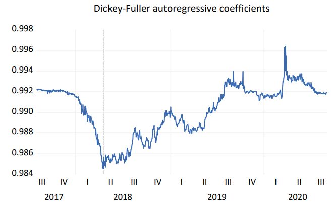
J. Risk Financial Manag. 2021, 14, 308 6 of 23
J. Risk Financial Manag. 2021, 14, x FOR PEER REVIEW 6 of 25
Figure 1. Architecture
Figure 1. Architecture ofof Research
Research Forecasting
Forecasting Model.
Model.
4.1.Volatility
4.1. VolatilityTime
Time Series
Series
Depending on
Depending on prior
prior knowledge
knowledge (conditional),
(conditional), the the time
time series
series depend
depend on on their
their past
past
value (autoregressive) and are shown (heteroscedasticity). The
value (autoregressive) and are shown (heteroscedasticity). The FOREX market volatilityFOREX market volatility
was found
was foundasaschanging
changingwith withtimetime (i.e.,
(i.e., “time
“time variation”),
variation”), with with clustering
clustering of volatility.
of volatility. In-
Interestingly, the associated volatility exponent for self-similarity
terestingly, the associated volatility exponent for self-similarity was discovered was discovered to increase
to in-
when when
crease high (resp., low) low)
high (resp., volatility clusters
volatility emerge
clusters emergein in
thetheseries
series(resp.,
(resp.,decreases).
decreases). TheThe
volatility exponent therefore would be approximately 0.5. On the
volatility exponent therefore would be approximately 0.5. On the contrary, assume that contrary, assume that
there are
there are some
some high
high volatility
volatility clusters
clusters in in the
the series
series (resp.,
(resp., low).
low). Therefore,
Therefore, nearly
nearly every
every
value in
value in the
the volatility
volatility series
series isis higher
higher (or (or lower)
lower) than
than the
the series
series mean.
mean. Consequently,
Consequently, the the
volatility series has increased (or decreased), with the result that it rises in self-similarity as
volatility series has increased (or decreased), with the result that it rises in self-similarity
well (resp., decreases).
as well (resp., decreases).
The major methods used for volatility modelling are the GARCH models. To record the
The major methods used for volatility modelling are the GARCH models. To record
volatility in the return series, GARCH methods are utilized. These models are frequently
the volatility in the return series, GARCH methods are utilized. These models are fre-
utilized in several fields of economic technology, particularly in the study of financial
quently utilized in several fields of economic technology, particularly in the study of fi-
time series. In addition, numerous empirical uses of modelling variance (volatility) of the
nancial time series. In addition, numerous empirical uses of modelling variance (volatil-
financial time series were introduced using the arch and GARCH models. Nevertheless, the
ity) of the financial time series were introduced using the arch and GARCH models. Nev-
GARCH could use leverage effect, which in one series represents a clustering of volatility
ertheless, the GARCH could use leverage effect, which in one series represents a cluster-
and leptokurtosis. This required the creation of new and extended models over GARCH,
ing of volatility and leptokurtosis. This required the creation of new and extended models
which resulted in new models with the E-GARCH Approach and ANN Backpropagation
over GARCH,model.
Combination which resulted in new models with the E-GARCH Approach and ANN
Backpropagation Combination model.
4.2. E-GARCH Model
4.2. E-GARCH Model
A conditional volatility model that can accommodate asymmetry is the EGARCH
modelA ofconditional volatility
(Nelson 1991). model that
The possibility can
that accommodate
EGARCH may beasymmetry is the EGARCH
made of a random coefficient
model of (Nelson 1991).The possibility that EGARCH
of nonlinear moving average (RCCNMA), in particular EGARCH (1), has may be made of a random coeffi-
been proven
cient of nonlinear
by (McAleer moving
and Hafner average
2014). Similar(RCCNMA), in particular
to the TGARCH, EGARCHGARCH
the exponential (1), hasmodel
been
proven
developed by (McAleer
by Nelsonandis toHafner
capture2014). Similar toofthe
consequences TGARCH,
leverage the (policies,
of shock exponential GARCH
information,
model developedand
news, incidents, by events)
Nelsonon is to
thecapture
financial consequences of leverage
market. It allows of shock
for the testing (policies, in-
of asymmetries.
formation, news, incidents, and events) on the financial market. It allows for the testing of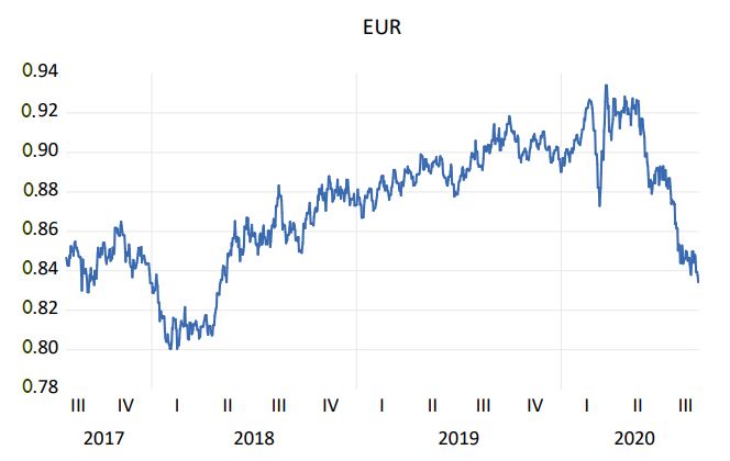
J. Risk Financial Manag. 2021, 14, 308                                                                                             7 of 23

                                         With good (bad) news, assets tend to enter a state of tranquility (turbulence), and volatility
                                         decreases (increases). This is done with the log of the variance series.
                                              One of the most common univariate asymmetric conditional volatility models is
                                         an exponential GARCH (or EGARCH) formulation. EGARCH may additionally accept
                                         leverage, the negative correlation between shocks in return and subsequent shocks. In
                                         addition to asymmetry, which captures the different effects on conditional volatility of
                                         positive and negative effects of equal magnitude, EGARCH can also accommodate leverage,
                                         which is the negative correlation between returns shocks and subsequent shocks to volatility.
                                         Depending on the proper limitations on model parameters, the EGARCH model can capture
                                         leverage. Let the conditional mean of financial returns be given as

                                                                              yt = E(yt /It−1 ) + ε t                                 (1)

                                         where yt = ∆ log Pt reflects the log difference in the price of FOREX, ( Pt ), It−1 is the data
                                         set at one moment, t − 1 and ε t is heteroscedastic conditionally.
                                              The EGARCH conditional variance ( p, q) model is specified as:
                                                                         q                 q              p
                                                                            u            u
                                                        log(ht ) = ψ + ∑ ηi p t−i + ∑ λi p t−i + ∑ θk log(ht−k )                      (2)
                                                                       i =1  h t −i i =1  h t − i k =1

                                              LHS is the series log of variance (ht ), which makes the leverage effect exponential
                                         rather than quadratic. This assures non-negative estimations. φ = constant, η = ARCH
                                         effects, λ = asymmetric effects and θ = GARCH effects.
                                              If λ1 = λ2 = · · · = 0 the model is symmetric.
                                              However, if λi < 0 it signifies terrible news (negative shocks) and generate large
                                         volatility then good news (positive shocks).

                                         4.2.1. Estimation Results
                                              The daily time-series data representing the capital market returns engaged in this
                                         training is obtained from Stock Exchange Reports for a certain period. The choice of
                                         the EGARCH framework is to accommodate the examination of conditional variance
                                         (volatility), asymmetric effect, and volatility persistence. The model for volatility using the
                                         EGARCH framework is specified as follows:

                                                                                        ∈ t−1 2           ∈ t−1

                                                               2              2
                                                             ϑt = ω + β in ϑt−1 + α             −     +γ                              (3)
                                                                                        ϑt − 1    x        ϑt − 1

                                         where, ω, β, α, γ are parameters constant. In ϑt2 is the one-term anticipation of volatility,
                                         and ω refers to the mean level, β is the parameter of persistence and α is the volatility
                                         clustering coefficient. Similarly, ϑt2−1 is the past variance and γ is the leverage effect.
                                               The EGARCH-in-mean model is a GARCH enhancement that imposes non-negativity
                                         constants on a market variable and enables a conditional variance to respond to innovations
                                         of various signs asymptomatically. If γ is negative, a leverage effect exists, implying that
                                         the bad news is more volatile than good news than expectations of similar magnitude.
                                         The negative value γ is often mentioned as the sign effect. If α positive, conditional
                                         volatility increases if the total value of the standardized residuals is greater (smaller).
                                         Where, α is the impression of magnitude. Interestingly, for related volatility series, the
                                         self-similarity exponent increases as high as (resp., low) volatility clusters are replaced by
                                         series (resp., decreases).

                                         4.2.2. Calculation of the Volatility Cluster Probability
                                               This section investigates how the volatility clusters may be evaluated for blocks of a
                                         certain size. The Hurst Exponent is usually regarded as a reliable indicator of the presence
                                         of trends. This exponent computation for each technique yields a different result as the
                                         period utilized and the length of underlying subintervals increase. As a consequence,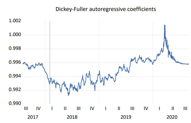
J. Risk Financial Manag. 2021, 14, 308 8 of 23
finding a unique Hurst exponent value is unattainable; therefore, calculating a unique
critical value is impossible.
Thus, Brownian Motion’s Hurst exponent volatility series is implied as a standard
to determine if the series contains a volatility cluster. Clusters match nicely with given
sectors including economic taxonomy (such as business sectors of the companies provided
by Forbes) and geoFigureical region (such as Asia and Europe). It may also detect assets
from clusters that are actively at work and dominate financial markets effectively. The
market activity might cause cluster changes. Here, I analyze how asset nodes are clustered
and analyze the evolution of clusters in the financial markets
More specifically, a set of Brownian movements was produced first via Monte Carlo
simulation. The exponents of their respective volatility ranges shall be computed for
every Brownian motion. The exponent of Hurst is greater than Hlim for the corresponding
volatility series as volatility clusters exist in the series. Then, measure the probability
of volatility clusters for subseries of a given length as the ratio between the number of
subseries with volatility clusters to the total amount of subseries of the given length. I test
it using artificial processes with volatility clusters to verify the likelihood of the clusters
of volatility.
4.3. Artificial Neural Networks
A huge nonlinear dynamic system, capable of carrying out extremely nonlinear, self-
learning and self-organizing operations, is an Artificial Neural Network (ANN). This experi-
ment employs the most frequently exploited business network, a neural background network.
4.3.1. Backpropagation Neural Networks
The backpropagation mechanism evaluates the weights of the connections between
the nodes in accordance with data formation results. This forming a minimized least
mean-square error measure of the actual, required, and estimated values from the output of
the neural network. Figure 2 depicts a three-layer backpropagation neural network. Initial
values are assigned to the connection weights. In addition, an error has backpropagated
J. Risk Financial Manag. 2021, 14, x FORacross a network to update weights between the actual and the expected output values.
PEER REVIEW 9 of 25
The monitored training process ensures that the mistake between the intended results and
the forecast is minimized.
SupervisedLearning
Figure2.2.Supervised
Figure LearningBack
BackPropagation
PropagationNeural
NeuralNetwork.
Network.
Theoretically, neural networks can imitate any data patterns with adequate training.
The BP-ANN training is as follows:
Before applying for predicting, the neural network must be trained. The neural network
Backpropagation is a supervised learning algorithm, for training Multilayer Percep-
In(n) Out(n)
is built on experience throughout the training phase based on the provided hypotheses.
For each neural network model, a hidden layer is used and the sigmoid function is the
tron’s (Artificial Neural Networks). Let and identify correspondingly
activation function.
the node input and output, as follows:
In n = m wmm Out m (4)
Outn = f (Inn + βn ) (5)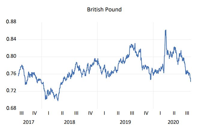
J. Risk Financial Manag. 2021, 14, 308                                                                                                 9 of 23

                                              The BP-ANN training is as follows:
                                              Backpropagation is a supervised learning algorithm, for training Multilayer Percep-
                                         tron’s (Artificial Neural Networks). Let In(n) and Out(n) identify correspondingly the
                                         node input and output, as follows:

                                                                                   Inn =    ∑ wmm Outm                                    (4)
                                                                                            m

                                                                                   Outn = f ( Inn + β n )                                 (5)
                                         where, wnm denotes the connecting weight from the mth node in the last node layer n, and

                                                                      f (net) = 2/1 − e−2net − 1                               (6)

                                              This signifies the node activation (“net” is the net input of the neuron), which causes
                                         nonlinearity to the neuron output, while β n is the bias input to the node of a specific
                                         unit with an active, consistent, nonzero value connection weight. The output error E is
                                         computed as follows:
                                                                               1                      2
                                                                             2N ∑   ∑( PNo − Out No )
                                                                        E=                                                        (7)
                                                                                  N o

                                         where N and o indicate the number of training items and the number of neurons in
                                         the output layer, respectively. The target PNo and output values Out No are represented
                                         accordingly. The training terminates if the error E falls below the threshold or degree
                                         of tolerance. This is the result of the error eo in the output layer and the error en in the
                                         concealed layer:
                                                                         eo = λ( PO − Outo ) f 0 (Outo )                           (8)
                                                                             en = λ∑ eo wmm f 0 (Outn )                                   (9)
                                                                                        m

                                         where the oth output node, real output in the output layer, current output in the hidden
                                         layer, Po , Outo , Outn and λ is anticipated to represent the output node and the activation
                                         function adjustable variable, respectively. It is worth noting that f 0 signifies the derivative
                                         of f . Error backpropagation is used to update the weights wmm and biases β(n) in both
                                         the output and hidden layers. The following equations are used to modify the weights
                                         and biases:
                                                                        wnm (k + 1) = wnm (k) + γe0 Outm                             (10)
                                                                             β m (k + 1) = β m (k) + γem                                (11)
                                         where the epoch number and the learning rate are denoted by k and γ, respectively. Neural
                                         networks are successful in forecasting very volatile financial variables that are difficult to
                                         anticipate using traditional statistical approaches, such as exchange rates and interest rates,
                                         according to empirical study.

                                         4.3.2. Hybrid Methodology (E-GARCH-NN)
                                               The system aims to incorporate the E-GARCH volatility method into neural networks
                                         (ANNs) that provide the functional flexibility to collect nonlinearity in financial information.
                                         First, the GM (1, 1)-GARCH model’s forecasting feature is used to continuously change the
                                         sequence of squared error terms. In addition, several estimated volatility methods are used
                                         for estimating the volatility, which is used to evaluate the performance of option-pricing
                                         models with the backpropagation ANN model.
                                               The model is specified as NN-EGARCH
                                                             p                 q    h                         √   i  s
                                               log σt2 = α + ∑ β i log σt2−1 + ∑ γ j δ(ε/σ )t− j + (ε/σ)t− j − z/π + ∑ ξ h ψ(zt λh )    (12)
                                                            i =1            j =1                                      h =1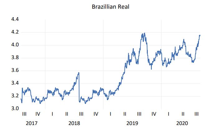
J. Risk Financial Manag. 2021, 14, 308                                                                                              10 of 23

                                                                       "                         "                        #!#−1
                                                                                             1       m
                                                           ψ(zt λh ) = 1 + exp λh,d,w +     ∑ ∑            λh,d,w Ztw−1                (13)
                                                                                            d =1 w =1
                                                                                                     q
                                                                           zt−d = [ε t−d − E(ε)]/        E ( ε2 )                      (14)

                                                                       (1/2)λh,d,w ∼ uni f orm[−1, +1]                                 (15)
                                         σt2is a function asymmetric of    ε t , log σt2
                                                                                  indicates natural logarithms, ψ(zt λh ) and zt−d is
                                         defined in Equations (12) and (13). The model utilizes a logarithmic design and square
                                         bracket terms to take into consideration the asymmetrical log ε effects.
                                               The conditional variance is not negative as a result of the logarithmic transformation.
                                         This study evaluates which model best represents financial time-series features and bet-
                                         ter predicts their future behavior since this allows market participants to decide on the
                                         projected future values. This study contributes to the direction by comparing the perfor-
                                         mance of the conventional E-GARCH model with the performance of the backpropagation
                                         neural network model in forecasting conditional variance of FOREX returns using cluster
                                         probability for currencies and cryptocurrencies.
                                               The research study can be evaluated with a wide range of real-time data. The data
                                         results must be noted and plotted for the analysis of the performance. The following
                                         methodology can be implemented and simulated on R-software or SPSS software, and
                                         the performance of the cryptocurrencies is compared with FOREX currencies for better
                                         comparative study, respectively.

                                         5. Results and Discussion
                                         5.1. Data and Preliminary Analysis
                                              The cryptocurrency data were composed of 2017 daily closing prices for the period of
                                         1 August 2017 to 31 August 2020. Almost all past research in this subject has focused on
                                         Bitcoin. This research focused on four cryptocurrencies: Ripple (XRP), Bitcoin, Ethereum,
                                         and Tether, which have the highest market capitalizations and a long history of data. These
                                         currencies and corresponding currency codes are listed in Table 1.

                                         Table 1. Cryptocurrencies.

                                                         Currency Name                                              Currency Code
                                                             Bitcoin                                                    BTC
                                                              Ripple                                                    XRP
                                                            Ethereum                                                    ETH
                                                              Tether                                                   USDT

                                              The top seven currencies were also taken for the study. The FOREX market operates
                                         24 h a day, 5 days a week where the different trading sessions of the Europe-an, Mexican,
                                         Australia, British, Brazilian, Saudi Arabia, and Japanese FOREX markets take place. The
                                         nature of FOREX trading has resulted in a high frequency market that has many changes
                                         of directions, which produce advantageous entry and exit points. The FOREX market is
                                         almost active the entire day, with price quotes rapidly changing. These FOREX currencies
                                         and their currency codes are listed in Table 2.
                                              Figure 3 illustrates the FX currencies return trajectories of the considered markets.
                                         Figure 3a states the time series of Australia. The Australian dollar shows a significant
                                         decrease in the middle of 2017, which broke through this range into the close of August
                                         with price quickly ducking back below in, early September trade. In 2020, the trend for
                                         the Australian dollar is rising, Australian dollar to average above 75 cents against the US
                                         dollar in 2020, about 5 cents higher than in 2019. Figure 3b portrays the Brazilian real time
                                         series. The Brazilian real illustrates the significant influence between the year 2019 and
J. Risk Financial Manag. 2021, 14, 308 11 of 23
2020. At the end of November 2020, one U.S. dollar could buy approximately 5.34 Brazilian
reals, approximately 1.7 pesos more than at the beginning of 2019.
Table 2. FOREX Currencies.
Currency Name Currency Code
Euro EUR
Australian Dollars AUD
Mexican Peso MXN
British Pound GBP
Brazilian Real BRL
J. Risk Financial Manag. 2021, 14, x FOR PEER REVIEW Saudi Riyal SAR 12 of 25
Japanese Yen JPY
(a) Australian Dollar (b) Brazilian Real
Figure
Figure3.3.Daily
Dailytime
timeseries
seriesof
ofFOREX
FOREXcurrencies
currencieswith
withAustralian
Australiandollar
dollarand
andBrazilian
Brazilian real.
real.
Figure4a
Figure 4astates
statesthat
thatthe
theBritish
Britishpound
poundvaries
variesin intime
timeseries
series in
in the
the years
years 2017–2020.
2017–2020. ItIt
hasaasignificant
has significantdecrease
decreasein in2017–2018.
2017–2018.Further,
Further,Figure
Figure4b 4bdenotes
denotesthe theEuro,
Euro,which
whichhashasaa
high impact in the year 2020. Figure 4c states the time series of the Mexican
high impact in the year 2020. Figure 4c states the time series of the Mexican peso; it impliespeso; it implies
thatfrom
that from2017–2019
2017–2019therethereisisaadecrease
decreasein inproduction
productionexceptexcept in
in2020.
2020.Figure
Figure4d4ddepicts
depictsthe
the
Saudi riyal time series. It shows that it looks like parallel production in the
Saudi riyal time series. It shows that it looks like parallel production in the years 2017, years 2017, 2018
and and
2018 2019.2019.
In comparison,
In comparison,the effect in 2020
the effect is less
in 2020 is significant.
less significant.
5.2. Descriptive Statistics
The descriptive statistics of foreign currencies are provided in Table 3 to define the
distributional characteristics of the daily return series of financial assets throughout the
research period. Table 3 examine the descriptive statistics in terms of the standard deviation
(SD), mean (X), kurtosis (K), and skewness (S), of the data. The data demonstrate that in
all cases, the returns are positively skewed rather than regularly distributed (except for
the Mexican peso, Australian dollar and Saudi riyal). Furthermore, the calculated kurtosis
was significantly greater than the normal distribution’s value, indicating that the data had
fewer than three in kurtosis. This means that it is dispersed normally.
(a) British Pound (b) European EUROFigure 4a states that the British pound varies in time series in the years 2017–2020. It
has a significant decrease in 2017–2018. Further, Figure 4b denotes the Euro, which has a
high impact in the year 2020. Figure 4c states the time series of the Mexican peso; it implies
that from 2017–2019 there is a decrease in production except in 2020. Figure 4d depicts the
J. Risk Financial Manag. 2021, 14, 308 12 of 23
Saudi riyal time series. It shows that it looks like parallel production in the years 2017,
2018 and 2019. In comparison, the effect in 2020 is less significant.
(a) British Pound (b) European EURO
(c) Mexican Peso (d) Saudi Riyal
Figure4.4.Daily
Figure Dailytime
time series
series of British pound,
pound,Euro,
Euro,Mexican
Mexicanpeso
pesoand
andSaudi
Saudiriyal.
riyal.
Table 3. Descriptive Statistics for FOREX Currencies.
Mean Median Maximum Minimum Std. Dev. Skewness Kurtosis
Euro 0.872696 0.8787 0.934 0.8004 0.031099 −0.39 −0.62
Mexican Peso 19.70841 19.16075 25.1039 17.6529 1.548699 1.64 1.98
British Pound 0.770294 0.76865 0.8622 0.6982 0.028363 −0.11 0.18
Australian Dollars 1.397557 1.40225 1.7253 1.2328 0.089557 0.44 0.46
Japanese Yen 109.5859 109.4716 114.193 102.2346 2.291237 0.03 −0.81
Brazilian Real 3.506903 3.325 4.1935 3.0889 0.319262 0.39 −1.36
Saudi Riyal 0.266577 0.2666 0.2667 0.2656 0.000121 −4.37 21.15
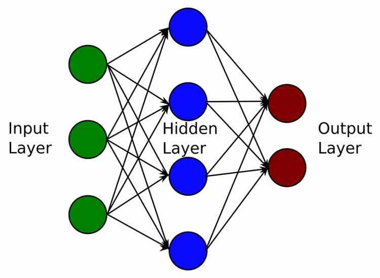
5.2.1. Volatility Clustering
Volatility is frequently estimated by the variance and default. The standard deviation is
the square root of the difference. With volatility persistence, volatility can shift expectations
on the stock market, with more uncertainty affecting investors’ decisions and desire to
investors because of risk exposure. Figure 5 shows the movements of daily market returns
of Bitcoin currency and traditional asset classes (equities, bonds, and cash) in the U.S.
market. Accordingly, Figure 5a denotes the return series of the FOREX market. This is
exhibiting volatility clustering persistence in their daily market returns. Figure 5b states
the return series of cryptocurrency bitcoin. This because their daily market returns series
volatility changes with time, or in other words, it is time-varying.sire to investors because of risk exposure. Figure 5 shows the movements of daily market
returns of Bitcoin currency and traditional asset classes (equities, bonds, and cash) in the
U.S. market. Accordingly, Figure 5a denotes the return series of the FOREX market. This
is exhibiting volatility clustering persistence in their daily market returns. Figure 5b states
J. Risk Financial Manag. 2021, 14, 308 13 of 23
the return series of cryptocurrency bitcoin. This because their daily market returns series
volatility changes with time, or in other words, it is time-varying.
J. Risk Financial Manag. 2021, 14, x FOR PEER REVIEW 14 of 25
(a) FOREX Market (b) Bitcoin
(c) Australian Dollar (d) Brazilian Real
Figure
Figure5.5.Volatility
VolatilityofofFOREX
FOREXCurrencies.
Currencies.
Figure5c5cillustrates
Figure illustratesthethevolatility
volatilityclustering
clusteringofofthe
theAustralian
Australiandollar.
dollar.Subsequently,
Subsequently,
Figure5d5dstates
Figure statesthe
theBrazilian
Brazilianreal
realvolatility
volatilitytime
timeseries
seriesofofFOREX
FOREXcurrencies.
currencies.TheTheobjective
objective
ofofthe
thework
workisistotodetermine
determinethe theoptimal
optimalGARCHGARCH
GARCHGARCHmodel modelforforthe
thereturn
returnseries
seriesafter
after
the clustering of volatility is validated using stationarity and return
the clustering of volatility is validated using stationarity and return series using ADF, series using ADF,
heteroscedasticity, and
heteroscedasticity, and pp
pp test,
test,and
andimpact
impact using thethe
using arch-lm test.test.
arch-lm As aAs result, in the in
a result, FOREX
the
market, the GARCH model is employed to represent the return
FOREX market, the GARCH model is employed to represent the return series volatility.series volatility.
Table4 4shows
Table showsthe theresults
resultsofofGARCH
GARCH(1,1)(1,1)models,
models,revealing
revealingthatthatthe
the GARCH
GARCH param-
param-
eterisissignificant
eter significantstatistically.
statistically.InInother
otherwords,
words,atatthethe0.05
0.05percent
percentlevel,
level,the
thecoefficients
coefficients
constant ( ω ), arch term ( α ), and GARCH term ( β ) are very significant. The calculated
constant (ω), arch term (α), and GARCH term (β) are very significant. The calculated
coefficient in the conditional variance equation is much larger than α.
coefficient in the conditional variance equation is much larger than α .
5.2.2. Augmented Dickey–Fuller (ADF) Test Coefficient Analysis
Table 4. Estimated Result of GARCH (1,1) Models.
The ADF is a unit root stationarity test. In a time-series analysis, unit roots can provide
Coefficientthe ADF test may be
unpredictable results. With serial correlation, GARCH
employed. (1,1)This test is
more powerful and can handle more complicated
Mean models than the Dickey–Fuller test.
0.87
Figure 6 states the unit root test of ADF test
(constant) µ analysis in the regression model of co-
efficients with the null hypothesis. Figure 6a,b
Variance α0states the Dickey–Fuller
−308.28autoregressive
Euro
coefficients for FOREX currencies of theα1 Australian dollar and Brazilian 8574.48 respective-ly.
real,
Figure 6c depicts the unit root test for the British Pound and illustrates the Dickey–Fuller
γ1 8574.48
test. This illustrates the Dickey–Fuller test with the least square support vector regression
β1 90.12
between the sample of 1 August 2017 to 31 August 2020. It contains Durbin Watson
Mean
statistics with a better coefficient of 0.871. Figure 6d states the Dickey–Fuller
19.71 (ADF) test of
(constant) µ
Euro in the regression model of coefficients with 0.976. Instantaneously, Figure 6e states the
Variance for the α0
Dickey–Fuller autoregressive coefficients 6712.63
Japanese yen, which relies on a regression
Mexican Peso
model with Durbin Watson statistics of α1 85,635.13 the Dickey–
0.909 coefficient. Figure 6f,g illustrates
Fuller autoregressive coefficients for the γ1Mexican peso and Saudi riyal, respectively. The
85,635.13
β1 40,008.81
Mean
0.77
(constant) µ
Variance α0 0.37
British Pound
α1 −0.01J. Risk Financial Manag. 2021, 14, 308 14 of 23
Mexican peso was tested with the sample R-Square and contains Durbin Watson statistics
with a better coefficient of 0.453.
Table 4. Estimated Result of GARCH (1,1) Models.
Coefficient GARCH (1,1)
Mean
0.87
(constant) µ
Variance α0 −308.28
Euro α1 8574.48
γ1 8574.48
β1 90.12
Mean
19.71
(constant) µ
Variance α0 6712.63
Mexican Peso α1 85,635.13
γ1 85,635.13
β1 40,008.81
Mean
0.77
(constant) µ
Variance α0 0.37
British Pound α1 −0.01
γ1 0.00
β1 1.14
Mean
1.40
(constant) µ
Variance α0 749.96
Australian Dollars α1 11,852.09
γ1 11,852.09
β1 517.28
Mean
109.59
(constant) µ
Variance α0 10,585.96
Japanese Yen
α1
γ1
β1 99,435.49
Mean
3.51
(constant) µ
Variance α0 0.05
Brazilian Real α1 0.02
γ1 −0.01
β1 0.92
Mean
0.27
(constant) µ
Saudi Riyal Variance α0 −2979.98
β1 7879.58tistics with a better coefficient of 0.871. Figure 6d states the Dickey–Fuller (ADF) test of
Euro in the regression model of coefficients with 0.976. Instantaneously, Figure 6e states
the Dickey–Fuller autoregressive coefficients for the Japanese yen, which relies on a re-
gression model with Durbin Watson statistics of 0.909 coefficient. Figure 6f,g illustrates
the Dickey–Fuller autoregressive coefficients for the Mexican peso and Saudi riyal, respec-
J. Risk Financial Manag. 2021, 14, 308 15 of 23
tively. The Mexican peso was tested with the sample R-Square and contains Durbin Wat-
son statistics with a better coefficient of 0.453.
J. Risk Financial Manag. 2021, 14, x FOR PEER REVIEW 16 of 25
(a) Australian Dollar (b) Brazilian Real
(c) British Pound (d) European Euro
(e) Japanese Yen (f) Mexican Peso
(g) Saudi Riyal
Figure
Figure 6. Dickey–Fuller
6. Dickey–Fuller autoregressive
autoregressive coefficients
coefficients for for seven
seven FOREX
FOREX Currencies.
Currencies.
5.3. Estimation of Asymmetric E-GARCH Volatility Persistence
This part of the paper describes the outcomes derived from fitting asymmetric and
symmetric return of the GARCH family models of Bitcoin currency and the U.S. tradi-
tional assets. This was implemented using Eviews. Tables 5–11 report the estimated coef-
ficients obtained by EGARCH (1,1) models.J. Risk Financial Manag. 2021, 14, 308 16 of 23
5.3. Estimation of Asymmetric E-GARCH Volatility Persistence
This part of the paper describes the outcomes derived from fitting asymmetric and
symmetric return of the GARCH family models of Bitcoin currency and the U.S. traditional
assets. This was implemented using Eviews. Tables 5–11 report the estimated coefficients
obtained by EGARCH (1,1) models.
Table 5. Estimated Result of E-GARCH Model for Australian Dollars Return Index during (2017–2020).
Dependent Variable: RETURN
Method: ML ARCH—Normal distribution (Marquardt/EViews legacy)
Date: 8 January 2021 Time: 12:27
Sample (adjusted): 3 August 2017 1 September 2020
Included observations: 1126 after adjustments
Convergence achieved after 13 iterations
Pre-sample variance: back cast (parameter = 0.7)
LOG(GARCH) = C(3) + C(4) * ABS(RESID(−1)/@SQRT(GARCH(−1))) + C(5) *
RESID(−1)/@SQRT(GARCH(−1)) + C(6) * LOG(GARCH(−1))
Variable Coefficient Std. Error z-Statistics Prob.
C 0.019058 0.013180 1.445896 0.1482
AR(1) 0.032232 0.029337 1.098675 0.2719
Variable Equation
C(3) −0.074659 0.014628 −5.103848 0.0000
C(4) 0.085551 0.015246 5.611323 0.0000
C(5) 0.014777 0.007826 1.888171 0.0590
C(6) 0.987601 0.003876 254.7958 0.0000
R-squared 0.001490 Mean dependent var 0.006802
Adjusted R-squared 0.000602 S.D. dependent var 0.485160
S.E. of regression 0.485014 Akaike info criterion 1.256707
Sum squared resid 264.4082 Schwarz criterion 1.283491
Log likelihood −701.5262 Hannan-Quinn criter 1.266828
Durbin-Watson stat 1.968187
Inverted AR Roots 0.03
Table 6. Estimated Result of E-GARCH Model for Brazilian Real Return Index during (2017–2020).
Dependent Variable: RETURN
Method: ML ARCH—Normal distribution (Marquardt/EViews legacy)
Date: 8 January 2021 Time: 12:32
Sample (adjusted): 3 August 2017 1 September 2020
Included observations: 1126 after adjustments
Convergence achieved after 24 iterations
Pre-sample variance: back cast (parameter = 0.7)
LOG(GARCH) = C(3) + C(4) * ABS(RESID(−1)/@SQRT(GARCH(−1))) + C(5) *
RESID(−1)/@SQRT(GARCH(−1)) + C(6) * LOG(GARCH(−1))
Variable Coefficient Std. Error z-Statistics Prob.
C 0.042660 0.021063 2.025395 0.0428
AR(1) −0.008846 0.042109 −0.210083 0.8336
Variable Equation
C(3) −1.227251 0.051303 −23.92181 0.0000
C(4) 0.502782 0.034177 14.71100 0.0000
C(5) −0.051102 0.026985 −1.893696 0.0583
C(6) −0.364374 0.048036 −7.585476 0.0000
R-squared 0.000160 Mean dependent var 0.024724
Adjusted R-squared −0.000730 S.D. dependent var 0.774829
S.E. of regression 0.775111 Akaike info criterion 2.261423
Sum squared resid 675.2965 Schwarz criterion 2.288207
Log likelihood −1267.181 Hannan-Quinn criter 2.271544
Durbin-Watson stat 2.069747
Inverted AR Roots −0.01J. Risk Financial Manag. 2021, 14, 308 17 of 23
Table 7. Estimated Result of E-GARCH Model for British Pound Return Index during (2017–2020).
Dependent Variable: RETURN
Method: ML ARCH—Normal distribution (Marquardt/EViews legacy)
Date: 8 January 2021 Time: 13:16
Sample (adjusted): 3 August 2017 1 September 2020
Included observations: 1126 after adjustments
Convergence achieved after 17 iterations
Pre-sample variance: back cast (parameter = 0.7)
LOG(GARCH) = C(3) + C(4) * ABS(RESID(−1)/@SQRT(GARCH(−1))) + C(5) *
RESID(−1)/@SQRT(GARCH(−1)) + C(6) * LOG(GARCH(−1))
Variable Coefficient Std. Error z-Statistics Prob.
C 0.001236 0.013481 0.091708 0.9269
AR(1) 0.000643 0.030951 0.020770 0.9834
Variable Equation
C(3) −2.410939 0.118084 −20.41719 0.0000
C(4) 0.295427 0.041449 7.127518 0.0000
C(5) −0.006186 0.028409 −0.217754 0.8276
C(6) −0.423517 0.070602 −5.998640 0.0000
R-squared 0.000029 Mean dependent var −0.001624
Adjusted R-squared −0.000860 S.D. dependent var 0.467410
S.E. of regression 0.467611 Akaike info criterion 1.287154
Sum squared resid 245.7744 Schwarz criterion 1.313937
Log likelihood −718.6675 Hannan-Quinn criter 1.297275
Durbin-Watson stat 1.888868
Inverted AR Roots 0.00
Table 8. Estimated Result of E-GARCH Model for Euro Return Index during (2017–2020).
Dependent Variable: RETURN
Method: ML ARCH—Normal distribution (Marquardt/EViews legacy)
Date: 8 January 2021 Time: 13:18
Sample (adjusted): 3 August 2017 1 September 2020
Included observations: 1126 after adjustments
Convergence achieved after 13 iterations
Pre-sample variance: back cast (parameter = 0.7)
LOG(GARCH) = C(3) + C(4) * ABS(RESID(−1)/@SQRT(GARCH(−1))) + C(5) *
RESID(−1)/@SQRT(GARCH(−1)) + C(6) * LOG(GARCH(−1))
Variable Coefficient Std. Error z-Statistics Prob.
C −0.002831 0.010908 −0.259526 0.7952
AR(1) 0.008867 0.032442 0.273307 0.7846
Variable Equation
C(3) −2.897089 0.236316 −12.25938 0.0000
C(4) 0.186335 0.049557 3.760047 0.0000
C(5) −0.070116 0.033627 −2.085136 0.0371
C(6) −0.369807 0.116715 −3.168454 0.0000
R-squared 0.000002 Mean dependent var −0.001184
Adjusted R-squared −0.000888 S.D. dependent var 0.365597
S.E. of regression 0.365759 Akaike info criterion 0.822749
Sum squared resid 150.3686 Schwarz criterion 0.849533
Log likelihood −457.2076 Hannan-Quinn criter 0.832870
Durbin-Watson stat 2.005011
Inverted AR Roots 0.01
Table 5 presents the estimated result of EGARCH (1, 1), the model for forex currencies
returns cryptocurrency. This implies that the asymmetric term’s coefficient is positive
(0.0147) and significant statistically at the 1% significance level. In exponential terms, C (5)
indicates that for the FTSE, bad news has a larger effect on the forex currencies’ volatility.
Table 6 illustrates the EGARCH (1, 1) estimated outcome of the model for forex
currencies Brazilian real returns cryptocurrency of Bitcoin. The overall findings reveal
higher leverage effects exist in the financial variables. This implies that the asymmetric
term coefficient is negative (−0.051) and significant statistically at the level of 1%. InYou can also read