Generative Models as Distributions of Functions - arXiv
←
→
Page content transcription
If your browser does not render page correctly, please read the page content below
Generative Models as Distributions of Functions

                                                   Emilien Dupont                         Yee Whye Teh                        Arnaud Doucet
                                                  University of Oxford                   University of Oxford                University of Oxford

                                                              Abstract
arXiv:2102.04776v3 [cs.LG] 19 Oct 2021

                                             Generative models are typically trained on
                                             grid-like data such as images. As a result,
                                             the size of these models usually scales directly
                                             with the underlying grid resolution. In this
                                             paper, we abandon discretized grids and in-
                                             stead parameterize individual data points by
                                             continuous functions. We then build gener-
                                             ative models by learning distributions over
                                             such functions. By treating data points as
                                             functions, we can abstract away from the spe-
                                             cific type of data we train on and construct
                                             models that are agnostic to discretization. To
                                             train our model, we use an adversarial ap-
                                             proach with a discriminator that acts on con-
                                             tinuous signals. Through experiments on a
                                             wide variety of data modalities including im-           Figure 1: By representing data as continuous func-
                                             ages, 3D shapes and climate data, we demon-             tions, we can use the same model to learn distributions
                                             strate that our model can learn rich distribu-          of images, 3D shapes and climate data, irrespective of
                                             tions of functions independently of data type           any underlying grid or discretization.
                                             and resolution.
                                                                                                     remarkable property that they are independent of sig-
                                                                                                     nal resolution [Park et al., 2019, Mescheder et al., 2018,
                                         1   Introduction                                            Chen and Zhang, 2019, Sitzmann et al., 2020].
                                                                                                     In this paper, we build generative models that inherit
                                         In generative modeling, data is often represented by        the attractive properties of implicit representations.
                                         discrete arrays. Images are represented by two dimen-       By framing generative modeling as learning distribu-
                                         sional grids of RGB values, 3D scenes are represented       tions of functions, we are able to build models that act
                                         by three dimensional voxel grids and audio as vectors       entirely on continuous spaces, independently of resolu-
                                         of discretely sampled waveforms. However, the true          tion. We achieve this by parameterizing a distribution
                                         underlying signal is often continuous. We can there-        over neural networks with a hypernetwork [Ha et al.,
                                         fore also consider representing such signals by contin-     2017] and training this distribution with an adversarial
                                         uous functions taking as input grid coordinates and         approach [Goodfellow et al., 2014], using a discrimina-
                                         returning features. In the case of images for exam-         tor that acts directly on sets of coordinates (e.g. pixel
                                         ple, we can define a function f : R2 → R3 mapping           locations) and features (e.g. RGB values). Crucially,
                                         pixel locations to RGB values using a neural network.       this allows us to train the model irrespective of any
                                         Such representations, typically referred to as implicit     underlying discretization or grid and avoid the curse
                                         neural representations, coordinate-based neural repre-      of discretization [Mescheder, 2020].
                                         sentations or neural function representations, have the
                                                                                                     Indeed, standard convolutional generative models act
                                                                                                     on discretized grids, such as images or voxels, and as a
                                                                                                     result scale quadratically or cubically with resolution,
                                                                                                     which quickly becomes intractable at high resolutions,
                                         Preprint. Under review.
                                                                                                     particularly in 3D [Park et al., 2019]. In contrast, our
Generative Models as Distributions of Functions

model learns distributions on continuous spaces and is           A core property of these representations is that they
agnostic to discretization. This allows us to not only           scale with signal complexity and not with signal res-
build models that act independently of resolution, but           olution [Sitzmann et al., 2020]. Indeed, the memory
also to learn distributions of functions on manifolds            required to store data scales quadratically with res-
where discretization can be difficult.                           olution for images and cubically for voxel grids. In
                                                                 contrast, for function representations, the memory re-
To validate our approach, we train generative mod-
                                                                 quirements scale directly with signal complexity: to
els on various image, 3D shape and climate datasets.
                                                                 represent a more complex signal, we would need to in-
Remarkably, we show that, using our framework, we
                                                                 crease the capacity of the function fθ , for example by
can learn rich function distributions on these var-
                                                                 increasing the number of layers of a neural network.
ied datasets using the same model. Further, by tak-
ing advantage of recent advances in representing high            Representing high frequency functions. Re-
frequency functions with neural networks [Mildenhall             cently, it has been shown that learning function rep-
et al., 2020, Tancik et al., 2020, Sitzmann et al., 2020],       resentations by minimizing equation (1) is biased to-
we also show that, unlike current approaches for gen-            wards learning low frequency functions [Mildenhall
erative modeling on continuous spaces [Garnelo et al.,           et al., 2020, Sitzmann et al., 2020, Tancik et al., 2020].
2018a, Mescheder et al., 2019, Kleineberg et al., 2020],         While several approaches have been proposed to al-
we are able to generate sharp and realistic samples.             leviate this problem, we use the random Fourier fea-
                                                                 ture (RFF) encoding proposed by Tancik et al. [2020]
2    Representing data as functions                              as it is not biased towards on axis variation (unlike
                                                                 Mildenhall et al. [2020]) and does not require spe-
In this section we review implicit neural representa-            cialized initialization (unlike Sitzmann et al. [2020]).
tions, using images as a guiding example for clarity.            Specifically, given a coordinate x ∈ Rd , the encoding
                                                                 function γ : Rd → R2m is defined as
Representing a single image with a function.
Let I be an image such that I[x, y] corresponds to the
                                                                                              cos(2πBx)

RGB value at pixel location (x, y). We are interested                            γ(x) =                   ,
                                                                                              sin(2πBx)
in representing this image by a function f : R2 → R3
where f (x, y) = (r, g, b) returns the RGB values at
                                                                 where B ∈ Rm×d is a (potentially learnable) ran-
pixel location (x, y). To achieve this, we parameterize
                                                                 dom matrix whose entries are typically sampled from
a function fθ by an MLP with weights θ, often referred
                                                                 N (0, σ 2 ). The number of frequencies m and the vari-
to as an implicit neural representation. We can then
                                                                 ance σ 2 of the entries of B are hyperparameters. To
learn this representation by minimizing
                  X                                              learn high frequency functions, we simply encode x be-
              min      kfθ (x, y) − I[x, y]k22 ,                 fore passing it through the MLP, fθ (γ(x)), and mini-
               θ                                                 mize equation (1).
                    x,y

where the sum is over all pixel locations. Remarkably,
the representation fθ is independent of the number of            3    Learning distributions of functions
pixels. The representation fθ therefore, unlike most
image representations, does not depend on the resolu-            In generative modeling, we are typically given a set
tion of the image [Mescheder et al., 2019, Park et al.,          of data, such as images, and are interested in approx-
2019, Sitzmann et al., 2020].                                    imating the distribution of this data. As we repre-
Representing general data with functions. The                    sent data points by functions, we would therefore like
above example with images can readily be extended to             to learn a distribution over functions. In the case of
more general data. Let x ∈ X denote coordinates and              images, standard generative models typically sample
y ∈ Y features and assume we are given a data point as           some noise and feed it through a neural network to
a set of coordinate and feature pairs {(xi , yi )}ni=1 . For     output n pixels [Goodfellow et al., 2014, Kingma and
an image for example, x = (x, y) corresponds to pixel            Welling, 2014, Rezende et al., 2014]. In contrast, we
locations, y = (r, g, b) corresponds to RGB values and           sample the weights of a neural network to obtain a
{(xi , yi )}ni=1 to the set of all pixel locations and RGB       function which we can probe at arbitrary coordinates.
values. Given a set of coordinates and their corre-              Such a representation allows us to operate entirely on
sponding features, we can learn a function fθ : X → Y            coordinates and features irrespective of any underlying
representing this data point by minimizing                       grid representation that may be available. To train the
                         n
                                                                 function distribution we use an adversarial approach
                                                                 and refer to our model as a Generative Adversarial
                         X
                   min          kfθ (xi ) − yi k22 .      (1)
                    θ
                          i=1
                                                                 Stochastic Process (GASP).
Emilien Dupont, Yee Whye Teh, Arnaud Doucet

3.1   Data representation

While our goal is to learn a distribution over functions,
we typically do not have access to the ground truth
functions representing the data. Instead, each data
point is typically given by some set of coordinates and
features s = {(xi , yi )}ni=1 . For an image for example,
we do not have access to a function mapping pixel lo-
cations to RGB values but to a collection of n pixels.        Figure 2: Diagram of a neural function distribution ar-
Such a set of coordinates and features corresponds to         chitecture. A latent vector z is mapped through a hy-
input/output pairs of a function, allowing us to learn        pernetwork gφ (in dashed lines) to obtain the weights
function distributions without operating directly on          of a function fθ (in solid lines) mapping coordinates x
the functions. A single data point then corresponds           to features y.
to a set of coordinates and features (e.g. an image is
a set of n pixels). We then assume a dataset is given
as samples s ∼ pdata (s) from a distribution over sets        ond function gφ : Z → Θ, itself with parameters φ,
of coordinate and feature pairs. Working with sets of         mapping latent variables to the weights θ of fθ (see
coordinates and features is very flexible - such a rep-       Figure 2). We can then sample from p(θ) by sampling
resentation is agnostic to whether the data originated        z ∼ p(z) and mapping z through gφ to obtain a set of
from a grid and at which resolution it was sampled.           weights θ = gφ (z). After sampling a function fθ , we
Crucially, formulating our problem entirely on sets also      then evaluate it at a set of coordinates {xi } to obtain
lets us split individual data points into subsets and         a set of generated features {yi } which can be used to
train on those. Specifically, given a single data point       train the model. Specifically, given a latent vector z
s = {(xi , yi )}ni=1 , such as a collection of n pixels, we   and a coordinate xi , we compute a generated feature
can randomly subsample K elements, e.g. we can se-            as yi = fgφ (z) (γ(xi )) where γ is an RFF encoding al-
lect K pixels among the n pixels in the entire image.         lowing us to learn high frequency functions.
Training on such subsets then removes any direct de-
pendence on the resolution of the data. For example,          3.3   Point cloud discriminator
when training on 3D shapes, instead of passing an en-
tire voxel grid to the model, we can train on subsets         In the GAN literature, discriminators are almost al-
of the voxel grid, leading to large memory savings (see       ways parameterized with convolutional neural net-
Section 5.2). This is not possible with standard con-         works (CNN). However, the data we consider may not
volutional models which are directly tied to the reso-        necessarily lie on a grid, in which case it is not possible
lution of the grid. Further, training on sets of coor-        to use convolutional discriminators. Further, convolu-
dinates and features allows us to model more exotic           tional discriminators scale directly with grid resolu-
data, such as distributions of functions on manifolds         tion (training a CNN on images at 2× the resolution
(see Section 5.3). Indeed, as long as we can define a         requires 4× the memory) which partially defeats the
coordinate system on the manifold (such as polar co-          purpose of using implicit representations.
ordinates on a sphere), our method applies.
                                                              As the core idea of our paper is to build genera-
                                                              tive models that are independent of discretization, we
3.2   Function generator                                      therefore cannot follow the naive approach of using
                                                              convolutional discriminators. Instead, our discrimi-
Learning distributions of functions with an adversarial       nator should be able to distinguish between real and
approach requires us to define a generator that gen-          fake sets of coordinate and feature pairs. Specifically,
erates fake functions and a discriminator that distin-        we need to define a function D which takes in an un-
guishes between real and fake functions. We define the        ordered set s and returns the probability that this set
function generator using the commonly applied hyper-          represents input/output pairs of a real function. We
network approach [Ha et al., 2017, Sitzmann et al.,           therefore need D to be permutation invariant with re-
2019, 2020, Anokhin et al., 2021, Skorokhodov et al.,         spect to the elements of the set s. The canonical choice
2021]. More specifically, we assume the structure (e.g.       for set functions is the PointNet [Qi et al., 2017] or
the number and width of layers) of the MLP fθ rep-            DeepSets [Zaheer et al., 2017] model family. However,
resenting a single data point is fixed. Learning a dis-       we experimented extensively with such functions and
tribution over functions fθ is then equivalent to learn-      found that they were not adequate for learning com-
ing a distribution over weights p(θ). The distribution        plex function distributions (see Section 3.5). Indeed,
p(θ) is defined by a latent distribution p(z) and a sec-      while the input to the discriminator is an unordered
Generative Models as Distributions of Functions

                                                            3.4   Training

                                                            We use the traditional (non saturating) GAN loss
                                                            [Goodfellow et al., 2014] for training and illustrate the
                                                            entire procedure for a single training step in Figure
                                                            4. To stabilize training, we define an equivalent of
                                                            the R1 penalty from Mescheder et al. [2018] for point
                                                            clouds. For images, R1 regularization corresponds to
                                                            penalizing the gradient norm of the discriminator with
Figure 3: Convolution neighborhood for regular con-         respect to the input image. For a set s = {(xi , yi )}ni=1 ,
volutions (left) and PointConv (right).                     we define the penalty as

                                                                         1                       1X
set s = {(xi , yi )}, there is an underlying notion of        R1 (s) =     k∇y1 ,...,yn D(s)k2 =     k∇yi D(s)k2 ,
                                                                         2                       2 y
distance between points xi in the coordinate space.                                                  i

We found that it is crucial to take this into account
                                                            that is we penalize the gradient norm of the discrimi-
when training models on complex datasets. Indeed, we
                                                            nator with respect to the features. Crucially, our entire
should not consider the coordinate and feature pairs
                                                            modeling procedure is then independent of discretiza-
as sets but rather as point clouds (i.e. sets with an
                                                            tion. Indeed, the generator, discriminator and loss all
underlying notion of distance).
                                                            act directly on continuous point clouds.
While several works have tackled the problem of point
cloud classification [Qi et al., 2017, Li et al., 2018,     3.5   How not to learn distributions of
Thomas et al., 2019], we leverage the PointConv                   functions
framework introduced by Wu et al. [2019] for sev-
eral reasons. Firstly, PointConv layers are transla-        In developing our model, we found that several ap-
tion equivariant (like regular convolutions) and per-       proaches which intuitively seem appropriate for learn-
mutation invariant by construction. Secondly, when          ing distributions of functions do not work in the con-
sampled on a regular grid, PointConv networks closely       text of generative modeling. We briefly describe these
match the performance of regular CNNs. Indeed, we           here and provide details and proofs in the appendix.
can loosely think of PointConv as a continuous equiv-
                                                            Set discriminators. As described in Section 3.3,
alent of CNNs and, as such, we can build PointConv
                                                            the canonical choice for set functions is the Point-
architectures that are analogous to typical discrimina-
                                                            Net/DeepSet model family [Qi et al., 2017, Zaheer
tor architectures.
                                                            et al., 2017]. Indeed, Kleineberg et al. [2020] use a sim-
Specifically, we assume we are given a set of features      ilar approach to ours to learn signed distance functions
fi ∈ Rcin at locations xi (we use fi to distinguish these   for 3D shapes using such a set discriminator. However,
hidden features of the network from input features yi ).    we found both theoretically and experimentally that
In contrast to regular convolutions, where the convolu-     PointNet/DeepSet functions were not suitable as dis-
tion kernels are only defined at certain grid locations,    criminators for complex function distributions (such as
the convolution filters in PointConv are parameterized      natural images). Indeed, these models do not directly
by an MLP, W : Rd → Rcout ×cin , mapping coordinates        take advantage of the metric on the space of coordi-
to kernel values. We can therefore evaluate the con-        nates, which we conjecture is crucial for learning rich
volution filters in the entire coordinate space. The        function distributions. In addition, we show in the ap-
PointConv operation at a point x is then defined as         pendix that the Lipschitz constant of set functions can
                          X                                 be very large, leading to unstable GAN training [Ar-
              fout (x) =      W (xi − x)fi ,                jovsky et al., 2017, Roth et al., 2017, Mescheder et al.,
                       xi ∈Nx                               2018]. We provide further theoretical and experimen-
                                                            tal insights on set discriminators in the appendix.
where Nx is a set of neighbors of x over which to per-
form the convolution (see Figure 3). Interestingly, this    Auto-decoders. A common method for embedding
neighborhood is found by a nearest neighbor search          functions into a latent space is the auto-decoder frame-
with respect to some metric on the coordinate space.        work used in DeepSDF [Park et al., 2019]. This frame-
We therefore have more flexibility in defining the con-     work and variants of it have been extensively used in
volution operation as we can choose the most appropri-      3D computer vision [Park et al., 2019, Sitzmann et al.,
ate notion of distance for the space we want to model       2019]. While auto-decoders excel at a variety of tasks,
(our implementation supports fast computation on the        we show in the appendix that the objective used to
GPU for any `p norm).                                       train these models is not appropriate for generative
Emilien Dupont, Yee Whye Teh, Arnaud Doucet

                   Generated data                          Real data                     Discriminator

         .                       .       .   .
         .                       .       .   .
         .                       .       .   .
                                                                       .   .     .   .
                                                                       .   .     .   .
                                                                       .   .     .   .

Figure 4: Training procedure for GASP: 1. Sample a function and evaluate it at a set of coordinate locations to
generate fake point cloud. 2. Convert real data sample to point cloud. 3. Discriminate between real and fake
point clouds.

modeling. We provide further analysis and experimen-        plicit representations for images. Crucially, these both
tal results on auto-decoders in the appendix.               use standard image convolutional discriminators and
                                                            as such do not inherit several advantages of implicit
While none of the above models were able to learn
                                                            representations: they are restricted to data lying on a
function distributions on complex datasets such as
                                                            grid and suffer from the curse of discretization. In con-
CelebAHQ, all of them worked well on MNIST. We
                                                            trast, GASP is entirely continuous and independent of
therefore believe that MNIST is not a meaningful
                                                            resolution and, as a result, we are able to train on a
benchmark for generative modeling of functions and
                                                            variety of data modalities.
encourage future research in this area to include ex-
periments on more complex datasets.                         Continuous models of 3D shape distributions.
                                                            Mescheder et al. [2019] use a VAE to learn distribu-
4   Related work                                            tions of occupancy networks for 3D shapes, while Chen
                                                            and Zhang [2019] train a GAN on embeddings of a
Implicit representations. Implicit representations          CNN autoencoder with an implicit function decoder.
were initially introduced in the context of evolutionary    Park et al. [2019], Atzmon and Lipman [2021] param-
algorithms as compositional pattern producing net-          eterize families of 3D shapes using the auto-decoder
works [Stanley, 2007]. In pioneering work, Ha [2016]        framework, which, as shown in Section 3.5, cannot be
built generative models of such networks for MNIST.         used for sampling. Kleineberg et al. [2020] use a set
Implicit representations for 3D geometry were initially     discriminator to learn distributions of signed distance
(and concurrently) proposed by [Park et al., 2019,          functions for 3D shape modeling. However, we show
Mescheder et al., 2019, Chen and Zhang, 2019]. A            both theoretically (see appendix) and empirically (see
large body of work has since taken advantage of these       Section 5) that using such a set discriminator severely
representations for inverse rendering [Sitzmann et al.,     limits the ability of the model to learn complex func-
2019, Mildenhall et al., 2020, Niemeyer et al., 2020,       tion distributions. Cai et al. [2020] represent functions
Yu et al., 2021], modeling dynamic scenes [Niemeyer         implicitly by gradient fields and use Langevin sam-
et al., 2019, Pumarola et al., 2021], modeling 3D scenes    pling to generate point clouds. Spurek et al. [2020]
[Atzmon and Lipman, 2020, Jiang et al., 2020, Gropp         learn a function mapping a latent vector to a point
et al., 2020] and superresolution [Chen et al., 2021].      cloud coordinate, which is used for point cloud gener-
                                                            ation. In addition, several recent works have tackled
Continuous models of image distributions. In                the problem of learning distributions of NeRF scenes
addition to the work of Ha [2016], neural processes         [Mildenhall et al., 2020], which are special cases of im-
[Garnelo et al., 2018a,b] are another family of mod-        plicit representations. This includes GRAF [Schwarz
els that can learn (conditional) distributions of im-       et al., 2020] which concatenates a latent vector to an
ages as functions. However, the focus of these is on        implicit representation and trains the model adversar-
uncertainty quantification and meta-learning rather         ially using a patch-based convolutional discriminator,
than generative modeling. Further, these models do          GIRAFFE [Niemeyer and Geiger, 2021] which adds
not scale to large datasets, although adding attention      compositionality to the generator and pi-GAN [Chan
[Kim et al., 2019] and translation equivariance [Gor-       et al., 2021] which models the generator using modu-
don et al., 2019] helps alleviate this. Gradient Ori-       lations to the hidden layer activations. Finally, while
gin Networks [Bond-Taylor and Willcocks, 2021] model        some of these works show basic results on small scale
distributions of implicit representations using an en-      image datasets, GASP is, to the best of our knowledge,
coder free model, instead using gradients of the la-        the first work to show how function distributions can
tents as an encoder. In concurrent work, Skorokhodov        be used to model a very general class of data, including
et al. [2021], Anokhin et al. [2021] use an adversarial     images, 3D shapes and data lying on manifolds.
approach to learn distributions of high frequency im-
Generative Models as Distributions of Functions

5     Experiments

We evaluate our model on CelebAHQ [Karras et al.,
2018] at 64×64 and 128×128 resolution, on 3D shapes
from the ShapeNet [Chang et al., 2015] chairs category
and on climate data from the ERA5 dataset [Hersbach
et al., 2019]. For all datasets we use the exact same
model except for the input and output dimensions of
the function representation and the parameters of the
Fourier features. Specifically, we use an MLP with 3
hidden layers of size 128 for the function representa-
tion and an MLP with 2 hidden layers of size 256 and
512 for the hypernetwork. Remarkably, we find that
such a simple architecture is sufficient for learning rich
distributions of images, 3D shapes and climate data.
The point cloud discriminator is loosely based on the
DCGAN architecture [Radford et al., 2015]. Specifi-          Figure 5: Samples from our model trained on Cele-
cally, for coordinates of dimension d, we use 3d neigh-      bAHQ 64 × 64 (top) and 128 × 128 (bottom). Each
bors for each PointConv layer and downsample points          image corresponds to a function which was sampled
by a factor of 2d at every pooling layer while doubling      from our model and then evaluated on the grid. To
the number of channels. We implemented our model             produce this figure we sampled 5 batches and chose
in PyTorch [Paszke et al., 2019] and performed all           the best batch by visual inspection.
training on a single 2080Ti GPU with 11GB of RAM.
The code can be found at https://github.com/
EmilienDupont/neural-function-distributions.

5.1   Images

We first evaluate our model on the task of image gener-
ation. To generate images, we sample a function from
the learned model and evaluate it on a grid. As can be
seen in in Figure 5, GASP produces sharp and realis-         Figure 6: Superresolution. The first column corre-
tic images both at 64 × 64 and 128 × 128 resolution.         sponds to the original resolution, the second column
While there are artifacts and occasionally poor sam-         to 4× the resolution and the third column to bicubic
ples (particularly at 128 × 128 resolution), the images      upsampling.
are generally convincing and show that the model has
learned a meaningful distribution of functions repre-        with a set discriminator (SD) (similar to Kleineberg
senting the data. To the best of our knowledge, this is      et al. [2020]) and a convolutional neural process (Con-
the first time data of this complexity has been modeled      vNP) [Gordon et al., 2019]. To the best of our knowl-
in an entirely continuous fashion.                           edge, these are the only other model families that can
                                                             learn generative models in a continuous manner, with-
As the representations we learn are independent of res-      out relying on a grid representation (which is required
olution, we can examine the continuity of GASP by            for regular CNNs). Results comparing all three models
generating images at higher resolutions than the data        on CelebAHQ 32 × 32 are shown in Figure 7. As can
on which it was trained. We show examples of this in         be seen, the baselines generate blurry and incoherent
Figure 6 by first sampling a function from our model,        samples, while our model is able to generate sharp, di-
evaluating it at the resolution on which it was trained      verse and plausible samples. Quantitatively, our model
and then evaluating it at a 4× higher resolution. As         (Table 1) outperforms all baselines, although it lags
can be seen, our model generates convincing 256 × 256        behind state of the art convolutional GANs special-
images even though it has only seen 64 × 64 images           ized to images [Lin et al., 2019].
during training, confirming the continuous nature of
GASP (see appendix for more examples).
                                                             5.2   3D scenes
We compare GASP against three baselines: a model
trained using the auto-decoder (AD) framework (sim-          To test the versatility and scalability of GASP, we also
ilar to DeepSDF [Park et al., 2019]), a model trained        train it on 3D shapes. To achieve this, we let the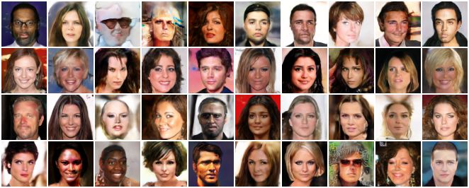
Emilien Dupont, Yee Whye Teh, Arnaud Doucet
AD
SD
GASP ConvNP

                                                           Figure 8: GPU memory consumption as a function of
                                                           the number of points K in voxel grid.

                                                                    163        323         643         1283
Figure 7: Baseline comparisons on CelebAHQ 32 × 32.
Note that the ConvNP model was trained on CelebA
(not CelebAHQ) and as such has a different crop.
                     CelebAHQ64   CelebAHQ128
              SD     236.82       -
              AD     117.80       -
              GASP   7.42         19.16
              Conv   4.00         5.74                     Figure 9: Evaluating the same function at different
                                                           resolutions. As samples from our model can be probed
Table 1: FID scores (lower is better) for various models
                                                           at arbitrary coordinates, we can increase the resolution
on CelebAHQ datasets, including a standard convolu-
                                                           to render smoother meshes.
tional image GAN [Lin et al., 2019].

function representation fθ : R3 → R map x, y, z co-
                                                           ON

ordinates to an occupancy value p (which is 0 if the
location is empty and 1 if it is part of an object).
To generate data, we follow the setup from Mescheder
                                                           SD

et al. [2019]. Specifically, we use the voxel grids from
Choy et al. [2016] representing the chairs category from
                                                           GASP

ShapeNet [Chang et al., 2015]. The dataset contains
6778 chairs each of dimension 323 . As each 3D model
is large (a set of 323 = 32, 768 points), we uniformly
subsample K = 4096 points from each object during          Figure 10: Samples from occupancy networks trained
training, which leads to large memory savings (Figure      as VAEs (ON), DeepSDF with set discriminators (SD)
8) and allows us to train with large batch sizes even on   and GASP trained on ShapeNet chairs. The top row
limited hardware. Crucially, this is not possible with     samples were taken from Mescheder et al. [2019] and
convolutional discriminators and is a key property of      the middle row samples from Kleineberg et al. [2020].
our model: we can train the model independently of
the resolution of the data.                                5.3    Climate data

In order to visualize results, we convert the functions    As we have formulated our framework entirely in terms
sampled from GASP to meshes we can render (see ap-         of continuous coordinates and features, we can easily
pendix for details). As can be seen in Figure 9, the       extend GASP to learning distributions of functions on
continuous nature of the data representation allows us     manifolds. We test this by training GASP on temper-
to sample our model at high resolutions to produce         ature measurements over the last 40 years from the
clean and smooth meshes. In Figure 10, we compare          ERA5 dataset [Hersbach et al., 2019], where each dat-
our model to two strong baselines for continuous 3D        apoint is a 46 × 90 grid of temperatures T measured
shape modeling: occupancy networks trained as VAEs         at evenly spaced latitudes λ and longitudes ϕ on the
[Mescheder et al., 2019] and DeepSDFs trained with         globe (see appendix for details). The dataset is com-
a set discriminator approach [Kleineberg et al., 2020].    posed of 8510 such grids measured at different points
As can be seen, GASP produces coherent and fairly di-      in time. We then model each datapoint by a function
verse samples, which are comparable to both baselines      f : S 2 → R mapping points on the sphere to tempera-
specialized to 3D shapes.                                  tures. We treat the temperature grids as i.i.d. samples
Generative Models as Distributions of Functions

                                                             plicable to a wide variety of data modalities, GASP
Samples

                                                             does not outperform state of the art specialized im-
                                                             age and 3D shape models. We strived for simplicity
                                                             when designing our model but hypothesize that stan-
                                                             dard GAN tricks [Karras et al., 2018, 2019, Arjovsky
                                                             et al., 2017, Brock et al., 2019] could help narrow
 Baseline

                                                             this gap in performance. In addition, we found that
                                                             training could be unstable, particularly when subsam-
                                                             pling points. On CelebAHQ for example, decreasing
                                                             the number of points per example also decreases the
Interpolation

                                                             quality of the generated images (see appendix for sam-
                                                             ples and failure examples), while the 3D model typi-
                                                             cally collapses to generating simple shapes (e.g. four
                                                             legged chairs) even if the data contains complex shapes
                                                             (e.g. office chairs). We conjecture that this is due
Figure 11: Results on climate data. The top row shows
                                                             to the nearest neighbor search in the discriminator:
samples from our model. The middle row shows com-
                                                             when subsampling points, a nearest neighbor may lie
parisons between GASP (on the right) and a baseline
                                                             very far from a query point, potentially leading to un-
(on the left) trained on a grid. As can be seen, the
                                                             stable training. More refined sampling methods and
baseline generates discontinuous samples at the grid
                                                             neighborhood searches should help improve stability.
boundary unlike GASP which produces smooth sam-
                                                             Finally, determining the neighborhood for the point
ples. The bottom row shows a latent interpolation cor-
                                                             cloud convolution can be expensive when a large num-
responding roughly to interpolating between summer
                                                             ber of points is used, although this could be mitigated
and winter in the northern hemisphere.
                                                             with faster neighbor search [Johnson et al., 2019].
                                                             Future work. As our model formulation is very
and therefore do not model any temporal correlation,
                                                             flexible, it would be interesting to apply GASP to
although we could in principle do this by adding time
                                                             geospatial [Jean et al., 2016], geological [Dupont et al.,
t as an input to our function.
                                                             2018], meteorological [Sønderby et al., 2020] or molec-
To ensure the coordinates lie on a manifold, we simply       ular [Wu et al., 2018] data which typically do not lie
convert the latitude-longitude pairs to spherical coor-      on a regular grid. In computer vision, we hope our
dinates before passing them to the function represen-        approach will help scale generative models to larger
tation, i.e. we set x = (cos λ cos ϕ, cos λ sin ϕ, sin λ).   datasets. While our model in its current form could
We note that, in contrast to standard discretized ap-        not scale to truly large datasets (such as room scale 3D
proaches which require complicated models to define          scenes), framing generative models entirely in terms of
convolutions on the sphere [Cohen et al., 2018, Esteves      coordinates and features could be a first step towards
et al., 2018], we only need a coordinate system on the       this. Indeed, while grid-based generative models cur-
manifold to learn distributions.                             rently outperform continuous models, we believe that,
                                                             at least for certain data modalities, continuous models
While models exist for learning conditional distribu-
                                                             will eventually surpass their discretized counterparts.
tions of functions on manifolds using Gaussian pro-
cesses [Borovitskiy et al., 2021, Jensen et al., 2020], we
are not aware of any work learning unconditional dis-        7    Conclusion
tributions of such functions for sampling. As a baseline
we therefore compare against a model trained directly        In this paper, we introduced GASP, a method for
on the grid of latitudes and longitudes (thereby ignor-      learning generative models that act entirely on con-
ing that the data comes from a manifold). Samples            tinuous spaces and as such are independent of signal
from our model as well as comparisons with the base-         discretization. We achieved this by learning distribu-
line and an example of interpolation in function space       tions over functions representing the data instead of
are shown in Figure 11. As can be seen, GASP gen-            learning distributions over the data directly. Through
erates plausible samples, smooth interpolations and,         experiments on images, 3D shapes and climate data,
unlike the baseline, is continuous across the sphere.        we showed that our model learns rich function distribu-
                                                             tions in an entirely continuous manner. We hope such
6               Scope, limitations and future work           a continuous approach will eventually enable genera-
                                                             tive modeling on data that is not currently tractable,
Limitations. While learning distributions of func-           either because discretization is expensive (such as in
tions gives rise to very flexible generative models ap-      3D) or difficult (such as on non-euclidean data).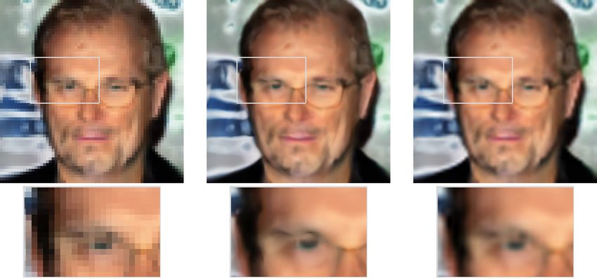
Emilien Dupont, Yee Whye Teh, Arnaud Doucet

Acknowledgements                                          16th European Conference, Glasgow, UK, August 23–
                                                          28, 2020, Proceedings, Part III 16, pages 364–381.
We thank William Zhang, Yuyang Shi, Jin Xu,               Springer, 2020.
Valentin De Bortoli, Jean-Francois Ton and Kaspar
Märtens for providing feedback on an early version       Eric R Chan, Marco Monteiro, Petr Kellnhofer, Ji-
of the paper. We also thank Charline Le Lan, Jean-        ajun Wu, and Gordon Wetzstein. pi-GAN: Periodic
Francois Ton and Bobby He for helpful discussions.        implicit generative adversarial networks for 3d-aware
We thank Yann Dubois for providing the ConvNP             image synthesis. In Proceedings of the IEEE/CVF
samples as well as helpful discussions around neural      Conference on Computer Vision and Pattern Recog-
processes. We thank Shahine Bouabid for help with         nition, pages 5799–5809, 2021.
the ERA5 climate data. Finally, we thank the anony-       Angel X Chang, Thomas Funkhouser, Leonidas
mous reviewers and the ML Collective for providing        Guibas, Pat Hanrahan, Qixing Huang, Zimo Li, Sil-
constructive feedback that helped us improve the pa-      vio Savarese, Manolis Savva, Shuran Song, Hao Su,
per. Emilien gratefully acknowledges his PhD funding      et al. Shapenet: An information-rich 3d model repos-
from Google DeepMind.                                     itory. arXiv preprint arXiv:1512.03012, 2015.

References                                                Yinbo Chen, Sifei Liu, and Xiaolong Wang. Learning
                                                          continuous image representation with local implicit
 Ivan Anokhin, Kirill Demochkin, Taras Khakhulin,         image function. In Proceedings of the IEEE/CVF
 Gleb Sterkin, Victor Lempitsky, and Denis Ko-            Conference on Computer Vision and Pattern Recog-
 rzhenkov.   Image generators with conditionally-         nition, pages 8628–8638, 2021.
 independent pixel synthesis. In Proceedings of the
 IEEE/CVF Conference on Computer Vision and               Zhiqin Chen and Hao Zhang. Learning implicit fields
 Pattern Recognition, pages 14278–14287, 2021.            for generative shape modeling. In Proceedings of
                                                          the IEEE/CVF Conference on Computer Vision and
 Martin Arjovsky, Soumith Chintala, and Léon Bot-        Pattern Recognition, pages 5939–5948, 2019.
 tou. Wasserstein generative adversarial networks.
 In International Conference on Machine Learning,         Christopher B Choy, Danfei Xu, JunYoung Gwak,
 pages 214–223, 2017.                                     Kevin Chen, and Silvio Savarese. 3d-r2n2: A uni-
                                                          fied approach for single and multi-view 3d object re-
 Matan Atzmon and Yaron Lipman. Sal: Sign agnostic        construction. In European Conference on Computer
 learning of shapes from raw data. In Proceedings of      Vision, pages 628–644. Springer, 2016.
 the IEEE/CVF Conference on Computer Vision and
 Pattern Recognition, pages 2565–2574, 2020.              Taco S Cohen, Mario Geiger, Jonas Köhler, and Max
                                                          Welling. Spherical cnns. In International Conference
 Matan Atzmon and Yaron Lipman. SALD: Sign                on Learning Representations, 2018.
 agnostic learning with derivatives. In International
 Conference on Learning Representations, 2021.            Emilien Dupont, Tuanfeng Zhang, Peter Tilke, Lin
                                                          Liang, and William Bailey. Generating realistic ge-
 Sam Bond-Taylor and Chris G Willcocks. Gradi-            ology conditioned on physical measurements with
 ent origin networks. In International Conference on      generative adversarial networks.   arXiv preprint
 Learning Representations, 2021.                          arXiv:1802.03065, 2018.
 Viacheslav Borovitskiy, Iskander Azangulov, Alexan-      Carlos Esteves, Christine Allen-Blanchette, Ameesh
 der Terenin, Peter Mostowsky, Marc Deisenroth, and       Makadia, and Kostas Daniilidis. Learning SO(3)
 Nicolas Durrande. Matérn Gaussian processes on          equivariant representations with spherical CNNs. In
 graphs. In International Conference on Artificial In-    Proceedings of the European Conference on Computer
 telligence and Statistics, pages 2593–2601, 2021.        Vision (ECCV), pages 52–68, 2018.
 Andrew Brock, Jeff Donahue, and Karen Simonyan.          Marta Garnelo, Dan Rosenbaum, Christopher Mad-
 Large scale gan training for high fidelity natural im-   dison, Tiago Ramalho, David Saxton, Murray Shana-
 age synthesis. In International Conference on Learn-     han, Yee Whye Teh, Danilo Rezende, and SM Ali Es-
 ing Representations, 2019.                               lami. Conditional neural processes. In International
                                                          Conference on Machine Learning, pages 1704–1713.
 Ruojin Cai, Guandao Yang, Hadar Averbuch-Elor,           PMLR, 2018a.
 Zekun Hao, Serge Belongie, Noah Snavely, and
 Bharath Hariharan. Learning gradient fields for          Marta Garnelo, Jonathan Schwarz, Dan Rosenbaum,
 shape generation. In Computer Vision–ECCV 2020:          Fabio Viola, Danilo J Rezende, SM Eslami, and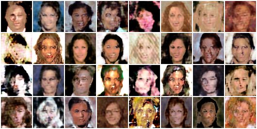
Generative Models as Distributions of Functions

Yee Whye Teh. Neural processes. arXiv preprint          Advances in Neural Information Processing Systems,
arXiv:1807.01622, 2018b.                                2020.

Ian J Goodfellow, Jean Pouget-Abadie, Mehdi Mirza,      Chiyu Jiang, Avneesh Sud, Ameesh Makadia, Jingwei
Bing Xu, David Warde-Farley, Sherjil Ozair, Aaron       Huang, Matthias Nießner, Thomas Funkhouser, et al.
Courville, and Yoshua Bengio. Generative adversar-      Local implicit grid representations for 3d scenes. In
ial networks. In Advances in Neural Information Pro-    Proceedings of the IEEE/CVF Conference on Com-
cessing Systems, 2014.                                  puter Vision and Pattern Recognition, pages 6001–
                                                        6010, 2020.
Jonathan Gordon, Wessel P Bruinsma, Andrew YK
Foong, James Requeima, Yann Dubois, and                 Jeff Johnson, Matthijs Douze, and Hervé Jégou.
Richard E Turner. Convolutional conditional neural      Billion-scale similarity search with GPUs. IEEE
processes. In International Conference on Learning      Transactions on Big Data, 2019.
Representations, 2019.
                                                        Tero Karras, Timo Aila, Samuli Laine, and Jaakko
Amos Gropp, Lior Yariv, Niv Haim, Matan Atzmon,         Lehtinen. Progressive growing of gans for improved
and Yaron Lipman. Implicit geometric regularization     quality, stability, and variation. In International Con-
for learning shapes. In International Conference on     ference on Learning Representations, 2018.
Machine Learning, pages 3789–3799. PMLR, 2020.
                                                        Tero Karras, Samuli Laine, and Timo Aila. A style-
Ishaan Gulrajani, Faruk Ahmed, Martin Arjovsky,         based generator architecture for generative adversar-
Vincent Dumoulin, and Aaron C Courville. Improved       ial networks. In Proceedings of the IEEE/CVF Con-
training of Wasserstein gans. In Advances in Neural     ference on Computer Vision and Pattern Recognition,
Information Processing Systems, pages 5767–5777,        pages 4401–4410, 2019.
2017.
                                                        Hyunjik Kim, Andriy Mnih, Jonathan Schwarz,
David Ha.     Generating large images from la-
                                                        Marta Garnelo, Ali Eslami, Dan Rosenbaum, Oriol
tent vectors.    blog.otoro.net, 2016.    URL
                                                        Vinyals, and Yee Whye Teh. Attentive neural pro-
https://blog.otoro.net/2016/04/01/
                                                        cesses. In International Conference on Learning Rep-
generating-large-images-from-latent-vectors/.
                                                        resentations, 2019.
David Ha, Andrew Dai, and Quoc V Le. HyperNet-
works. International Conference on Learning Repre-      Diederik P Kingma and Max Welling. Auto-encoding
sentations, 2017.                                       variational Bayes. In International Conference on
                                                        Learning Representations, 2014.
H. Hersbach, B. Bell, P. Berrisford, G. Bia-
vati, A. Horányi, J. Muñoz Sabater, J. Nicolas,       Marian Kleineberg, Matthias Fey, and Frank We-
C. Peubey, R. Radu, I. Rozum, D. Schepers,              ichert. Adversarial generation of continuous implicit
A. Simmons, C. Soci, D. Dee, and J-N. Thépaut.         shape representations. In Eurographics - Short Pa-
ERA5 monthly averaged data on single levels from        pers, 2020.
1979 to present. Copernicus Climate Change Ser-
                                                        Juho Lee, Yoonho Lee, Jungtaek Kim, Adam
vice (C3S) Climate Data Store (CDS). https://
                                                        Kosiorek, Seungjin Choi, and Yee Whye Teh.
cds.climate.copernicus.eu/cdsapp#!/dataset/
                                                        Set transformer: A framework for attention-based
reanalysis-era5-single-levels-monthly-means
                                                        permutation-invariant neural networks. In Interna-
(Accessed 27-09-2021), 2019.
                                                        tional Conference on Machine Learning, pages 3744–
Sergey Ioffe and Christian Szegedy. Batch normaliza-    3753. PMLR, 2019.
tion: Accelerating deep network training by reducing
internal covariate shift. In International Conference   Yangyan Li, Rui Bu, Mingchao Sun, Wei Wu, Xinhan
on Machine Learning, pages 448–456. PMLR, 2015.         Di, and Baoquan Chen. PointCNN: Convolution on
                                                        x-transformed points. Advances in Neural Informa-
Neal Jean, Marshall Burke, Michael Xie, W Matthew       tion Processing Systems, 31:820–830, 2018.
Davis, David B Lobell, and Stefano Ermon. Combin-
ing satellite imagery and machine learning to predict   Chieh Hubert Lin, Chia-Che Chang, Yu-Sheng Chen,
poverty. Science, 353(6301):790–794, 2016.              Da-Cheng Juan, Wei Wei, and Hwann-Tzong Chen.
                                                        Coco-gan: Generation by parts via conditional coor-
Kristopher Jensen, Ta-Chu Kao, Marco Tripodi, and       dinating. In Proceedings of the IEEE/CVF Interna-
Guillaume Hennequin. Manifold GPLVMs for discov-        tional Conference on Computer Vision, pages 4512–
ering non-euclidean latent structure in neural data.    4521, 2019.
Emilien Dupont, Yee Whye Teh, Arnaud Doucet
William E Lorensen and Harvey E Cline. Marching Killeen, Zeming Lin, Natalia Gimelshein, Luca
cubes: A high resolution 3d surface construction al- Antiga, et al. Pytorch: An imperative style, high-
gorithm. ACM Siggraph Computer Graphics, 21(4): performance deep learning library. Advances in Neu-
163–169, 1987. ral Information Processing Systems, 32:8026–8037,
2019.
Lars Mescheder, Andreas Geiger, and Sebastian
Nowozin. Which training methods for gans do actu- Albert Pumarola, Enric Corona, Gerard Pons-Moll,
ally converge? In International Conference on Ma- and Francesc Moreno-Noguer. D-nerf: Neural ra-
chine learning, pages 3481–3490, 2018. diance fields for dynamic scenes. In Proceedings of
the IEEE/CVF Conference on Computer Vision and
Lars Mescheder, Michael Oechsle, Michael Niemeyer, Pattern Recognition, pages 10318–10327, 2021.
Sebastian Nowozin, and Andreas Geiger. Occupancy
networks: Learning 3d reconstruction in function Charles R Qi, Hao Su, Kaichun Mo, and Leonidas J
space. In Proceedings of the IEEE/CVF Conference Guibas. Pointnet: Deep learning on point sets for 3d
on Computer Vision and Pattern Recognition, pages classification and segmentation. In Proceedings of the
4460–4470, 2019. IEEE conference on Computer Vision and Pattern
Eecognition, pages 652–660, 2017.
Lars Morten Mescheder. Stability and Expressiveness
of Deep Generative Models. PhD thesis, Universität Alec Radford, Luke Metz, and Soumith Chintala. Un-
Tübingen, 2020. supervised representation learning with deep convolu-
tional generative adversarial networks. arXiv preprint
Ben Mildenhall, Pratul P Srinivasan, Matthew Tan- arXiv:1511.06434, 2015.
cik, Jonathan T Barron, Ravi Ramamoorthi, and Ren
Ng. Nerf: Representing scenes as neural radiance Nikhila Ravi, Jeremy Reizenstein, David Novotny,
fields for view synthesis. In European Conference on Taylor Gordon, Wan-Yen Lo, Justin Johnson, and
Computer Vision, pages 405–421, 2020. Georgia Gkioxari. Accelerating 3d deep learning with
pytorch3d. arXiv preprint arXiv:2007.08501, 2020.
Takeru Miyato, Toshiki Kataoka, Masanori Koyama,
Danilo Jimenez Rezende, Shakir Mohamed, and
and Yuichi Yoshida. Spectral normalization for gen-
Daan Wierstra. Stochastic backpropagation and ap-
erative adversarial networks. In International Con-
proximate inference in deep generative models. In In-
ference on Learning Representations, 2018.
ternational Conference on Machine Learning, pages
Michael Niemeyer and Andreas Geiger. GIRAFFE: 1278–1286. PMLR, 2014.
Representing scenes as compositional generative neu- Kevin Roth, Aurelien Lucchi, Sebastian Nowozin,
ral feature fields. In Proceedings of the IEEE/CVF and Thomas Hofmann. Stabilizing training of gener-
Conference on Computer Vision and Pattern Recog- ative adversarial networks through regularization. In
nition, pages 11453–11464, 2021. Advances in Neural Information Processing Systems,
Michael Niemeyer, Lars Mescheder, Michael Oechsle, pages 2018–2028, 2017.
and Andreas Geiger. Occupancy flow: 4d reconstruc- Katja Schwarz, Yiyi Liao, Michael Niemeyer, and An-
tion by learning particle dynamics. In Proceedings dreas Geiger. GRAF: Generative radiance fields for
of the IEEE/CVF International Conference on Com- 3d-aware image synthesis. Advances in Neural Infor-
puter Vision, pages 5379–5389, 2019. mation Processing Systems, 33, 2020.
Michael Niemeyer, Lars Mescheder, Michael Oechsle, Maximilian Seitzer. pytorch-fid: FID Score
and Andreas Geiger. Differentiable volumetric ren- for PyTorch. https://github.com/mseitzer/
dering: Learning implicit 3d representations without pytorch-fid, August 2020. Version 0.1.1.
3d supervision. In Proc. IEEE Conf. on Computer
Vision and Pattern Recognition (CVPR), 2020. Vincent Sitzmann, Michael Zollhöfer, and Gordon
Wetzstein. Scene representation networks: Continu-
Jeong Joon Park, Peter Florence, Julian Straub, ous 3d-structure-aware neural scene representations.
Richard Newcombe, and Steven Lovegrove. Deepsdf: In Advances in Neural Information Processing Sys-
Learning continuous signed distance functions for tems, pages 1121–1132, 2019.
shape representation. In Proceedings of the IEEE
Conference on Computer Vision and Pattern Recog- Vincent Sitzmann, Julien Martel, Alexander
nition, pages 165–174, 2019. Bergman, David Lindell, and Gordon Wetzstein.
Implicit neural representations with periodic acti-
Adam Paszke, Sam Gross, Francisco Massa, Adam vation functions. Advances in Neural Information
Lerer, James Bradbury, Gregory Chanan, Trevor Processing Systems, 33, 2020.Generative Models as Distributions of Functions
Ivan Skorokhodov, Savva Ignatyev, and Mohamed or few images. In Proceedings of the IEEE/CVF Con-
Elhoseiny. Adversarial generation of continuous im- ference on Computer Vision and Pattern Recognition,
ages. In Proceedings of the IEEE/CVF Conference pages 4578–4587, 2021.
on Computer Vision and Pattern Recognition, pages
10753–10764, 2021. Manzil Zaheer, Satwik Kottur, Siamak Ravan-
bakhsh, Barnabas Poczos, Russ R Salakhutdinov,
Casper Kaae Sønderby, Lasse Espeholt, Jonathan and Alexander J Smola. Deep sets. In Advances in
Heek, Mostafa Dehghani, Avital Oliver, Tim Sali- Neural Information Processing Systems, pages 3391–
mans, Shreya Agrawal, Jason Hickey, and Nal Kalch- 3401, 2017.
brenner. Metnet: A neural weather model for precip-
itation forecasting. arXiv preprint arXiv:2003.12140,
2020.
Przemyslaw Spurek, Sebastian Winczowski, Jacek
Tabor, Maciej Zamorski, Maciej Zieba, and Tomasz
Trzcinski. Hypernetwork approach to generating
point clouds. In International Conference on Ma-
chine Learning, pages 9099–9108, 2020.
Kenneth O Stanley. Compositional pattern produc-
ing networks: A novel abstraction of development.
Genetic programming and evolvable machines, 8(2):
131–162, 2007.
Karl Stelzner, Kristian Kersting, and Adam R Ko-
siorek. Generative adversarial set transformers. In
Workshop on Object-Oriented Learning at ICML, vol-
ume 2020, 2020.
Matthew Tancik, Pratul P Srinivasan, Ben Milden-
hall, Sara Fridovich-Keil, Nithin Raghavan, Utkarsh
Singhal, Ravi Ramamoorthi, Jonathan T Barron, and
Ren Ng. Fourier features let networks learn high
frequency functions in low dimensional domains. In
Advances in Neural Information Processing Systems,
2020.
Hugues Thomas, Charles R Qi, Jean-Emmanuel De-
schaud, Beatriz Marcotegui, François Goulette, and
Leonidas J Guibas. Kpconv: Flexible and deformable
convolution for point clouds. In Proceedings of the
IEEE/CVF International Conference on Computer
Vision, pages 6411–6420, 2019.
Wenxuan Wu, Zhongang Qi, and Li Fuxin. Point-
conv: Deep convolutional networks on 3d point
clouds. In Proceedings of the IEEE Conference on
Computer Vision and Pattern Recognition, pages
9621–9630, 2019.
Zhenqin Wu, Bharath Ramsundar, Evan N Feinberg,
Joseph Gomes, Caleb Geniesse, Aneesh S Pappu,
Karl Leswing, and Vijay Pande. Moleculenet: a
benchmark for molecular machine learning. Chem-
ical Science, 9(2):513–530, 2018.
Alex Yu, Vickie Ye, Matthew Tancik, and Angjoo
Kanazawa. pixelnerf: Neural radiance fields from oneEmilien Dupont, Yee Whye Teh, Arnaud Doucet A Experimental details In this section we provide experimental details necessary to reproduce all results in the paper. All the models were implemented in PyTorch Paszke et al. [2019] and trained on a single 2080Ti GPU with 11GB of RAM. The code to reproduce all experiments can be found at https://github.com/EmilienDupont/ neural-function-distributions. A.1 GASP experiments For all experiments (images, 3D shapes and climate data), we parameterized fθ by an MLP with 3 hidden layers, each with 128 units. We used a latent dimension of 64 and an MLP with 2 hidden layers of dimension 256 and 512 for the hypernetwork gφ . We normalized all coordinates to lie in [−1, 1]d and all features to lie in [−1, 1]k . We used LeakyReLU non-linearities both in the generator and discriminator. The final output of the function representation was followed by a tanh non-linearity. For the point cloud discriminator, we used 3d neighbors in each convolution layer and followed every convolution by an average pooling layer reducing the number of points by 2d . We applied a sigmoid as the final non-linearity. We used an MLP with 4 hidden layers each of size 16 to parameterize all weight MLPs. Unless stated otherwise, we use Adam with a learning rate of 1e-4 for the hypernetwork weights and 4e-4 for the discriminator weights with β1 = 0.5 and β2 = 0.999 as is standard for GAN training. For each dataset, we trained for a large number of epochs and chose the best model by visual inspection. MNIST • Dimensions: d = 2, k = 1 • Fourier features: m = 128, σ = 1 • Discriminator channels: 64, 128, 256 • Batch size: 128 • Epochs: 150 CelebAHQ 64x64 • Dimensions: d = 2, k = 3 • Fourier features: m = 128, σ = 2 • Discriminator channels: 64, 128, 256, 512 • Batch size: 64 • Epochs: 300 CelebAHQ 128x128 • Dimensions: d = 2, k = 3 • Fourier features: m = 128, σ = 3 • Discriminator channels: 64, 128, 256, 512, 1024 • Batch size: 22 • Epochs: 70 ShapeNet voxels
Generative Models as Distributions of Functions

  • Dimensions: d = 3, k = 1
  • Fourier features: None
  • Discriminator channels: 32, 64, 128, 256
  • Batch size: 24
  • Learning rates: Generator 2e-5, Discriminator 8e-5
  • Epochs: 200

ERA5 climate data

  • Dimensions: d = 2, k = 1
  • Fourier features: m = 128, σ = 2
  • Discriminator channels: 64, 128, 256, 512
  • Batch size: 64
  • Epochs: 300

A.2   Things we tried that didn’t work
  • We initially let the function representation fθ have 2 hidden layers of size 256, instead of 3 layers of size 128.
    However, we found that this did not work well, particularly for more complex datasets. We hypothesize
    that this is because the number of weights in a single 256 → 256 linear layer is 4× the number of weights in
    a single 128 → 128 layer. As such, the number of weights in four 128 → 128 layers is the same as a single
    256 → 256, even though such a 4-layer network would be much more expressive. Since the hypernetwork
    needs to output all the weights of the function representation, the final layer of the hypernetwork will be
    extremely large if the number of function weights is large. It is therefore important to make the network as
    expressive as possible with as few weights as possible, i.e. by making the network thinner and deeper.
  • As the paper introducing the R1 penalty [Mescheder et al., 2018] does not use batchnorm [Ioffe and Szegedy,
    2015] in the discriminator, we initially ran experiments without using batchnorm. However, we found that
    using batchnorm both in the weight MLPs and between PointConv layers was crucial for stable training.
    We hypothesize that this is because using standard initializations for the weights of PointConv layers would
    result in PointConv outputs (which correspond to the weights in regular convolutions) that are large. Adding
    batchnorm fixed this initialization issue and resulted in stable training.
  • In the PointConv paper, it was shown that the number of hidden layers in the weight MLPs does not
    significantly affect classification performance [Wu et al., 2019]. We therefore initially experimented with
    single hidden layer MLPs for the weights. However, we found that it is crucial to use deep networks for the
    weight MLPs in order to build discriminators that are expressive enough for the datasets we consider.
  • We experimented with learning the frequencies of the Fourier features (i.e. learning B) but found that this
    did not significantly boost performance and generally resulted in slower training.

A.3   ERA5 climate data

We extracted the data used for the climate experiments from the ERA5 database [Hersbach et al., 2019]. Specif-
ically, we used the monthly averaged surface temperature at 2m, with reanalysis by hour of day. Each data
point then corresponds to a set of temperature measurements on a 721 x 1440 grid (i.e. 721 latitudes and 1440
longitudes) across the entire globe (corresponding to measurements every 0.25 degrees). For our experiments,
we subsample this grid by a factor of 16 to obtain grids of size 46 x 90. For each month, there are a total of
24 grids, corresponding to each hour of the day. The dataset is then composed of temperature measurements
for all months between January 1979 and December 2020, for a total of 12096 datapoints. We randomly split
this dataset into a train set containing 8510 grids, a validation set containing 1166 grids and a test set contain-
ing 2420 grids. Finally, we normalize the data to lie in [0, 1] with the lowest temperature recorded since 1979
corresponding to 0 and the highest temperature to 1.
Emilien Dupont, Yee Whye Teh, Arnaud Doucet
Figure 12: Left: Samples from an auto-decoder model trained on MNIST. Right: Samples from an auto-decoder
model trained on CelebAHQ 32 × 32.
A.4 Quantitative experiments
We computed FID scores using the pytorch-fid library [Seitzer, 2020]. We generated 30k samples for both
CelebAHQ 64 × 64 and 128 × 128 and used default settings for all hyperparameters. We note that the FID
scores for the convolutional baselines in the main paper were computed on CelebA (not the HQ version) and
are therefore not directly comparable with our model. However, convolutional GANs would also outperform our
model on CelebAHQ.
A.5 Rendering 3D shapes
In order to visualize results for the 3D experiments, we convert the functions sampled from GASP to meshes we
can render. To achieve this, we first sample a function from our model and evaluate it on a high resolution grid
(usually 1283 ). We then threshold the values of this grid at 0.5 (we found the model was robust to choices of
threshold) so voxels with values above the threshold are occupied while the rest are empty. Finally, we use the
marching cubes algorithm [Lorensen and Cline, 1987] to convert the grid to a 3D mesh which we render with
PyTorch3D [Ravi et al., 2020].
B Models that are not suitable for learning function distributions
B.1 Auto-decoders
We briefly introduce auto-decoder models following the setup in [Park et al., 2019] and describe why they are not
suitable as generative models. As in the GASP case, we assume we are given a dataset of N samples {s(i) }N i=1
(where each sample s(i) is a set). We then associate a latent vector z(i) with each sample s(i) . We further
parameterize a probabilistic model pθ (s(i) |z(i) ) (similar to the decoder in variational autoencoders) by a neural
network with learnable parameters θ (typically returning the mean of a Gaussian with fixed variance). The
optimal parameters are then estimated as
N
X
arg max log pθ (s(i) |z(i) ) + log p(z(i) ),
θ,{z(i) }
i=1
where p(z) is a (typically Gaussian) prior over the z(i) ’s. Crucially the latents vectors z(i) are themselves learnable
and optimized. However, maximizing log p(z(i) ) ∝ −kz(i) k2 does not encourage the z(i) ’s to be distributed
according to the prior, but only encourages them to have a small norm. Note that this is because we are
optimizing the samples and not the parameters of the Gaussian prior. As such, after training, the z(i) ’s are
unlikely to be distributed according to the prior. Sampling from the prior to generate new samples from the
model will therefore not work.
We hypothesize that this is why the prior is required to have very low variance for the auto-decoder model to work
well [Park et al., 2019]. Indeed, if the norm of the z(i) ’s is so small that they are barely changed during training,
they will remain close to their initial Gaussian distribution. While this trick is sufficient to learn distributionsYou can also read