Trajectron++: Dynamically-Feasible Trajectory Forecasting With Heterogeneous Data
←
→
Page content transcription
If your browser does not render page correctly, please read the page content below
Trajectron++: Dynamically-Feasible Trajectory
arXiv:2001.03093v3 [cs.RO] 1 Jun 2020
                                             Forecasting With Heterogeneous Data

                                                Tim Salzmann?†1 , Boris Ivanovic?1 , Punarjay Chakravarty2 , and
                                                                        Marco Pavone1
                                                           1
                                                               Autonomous Systems Lab, Stanford University
                                                                {timsal, borisi, pavone}@stanford.edu
                                                                         2
                                                                           Ford Greenfield Labs
                                                                           pchakra5@ford.com

                                                Abstract. Reasoning about human motion is an important prerequisite
                                                to safe and socially-aware robotic navigation. As a result, multi-agent be-
                                                havior prediction has become a core component of modern human-robot
                                                interactive systems, such as self-driving cars. While there exist many
                                                methods for trajectory forecasting, most do not enforce dynamic con-
                                                straints and do not account for environmental information (e.g., maps).
                                                Towards this end, we present Trajectron++, a modular, graph-structured
                                                recurrent model that forecasts the trajectories of a general number of di-
                                                verse agents while incorporating agent dynamics and heterogeneous data
                                                (e.g., semantic maps). Trajectron++ is designed to be tightly integrated
                                                with robotic planning and control frameworks; for example, it can pro-
                                                duce predictions that are optionally conditioned on ego-agent motion
                                                plans. We demonstrate its performance on several challenging real-world
                                                trajectory forecasting datasets, outperforming a wide array of state-of-
                                                the-art deterministic and generative methods.

                                                Keywords: Trajectory Forecasting, Spatiotemporal Graph Modeling,
                                                Human-Robot Interaction, Autonomous Driving

                                1             Introduction
                                Predicting the future behavior of humans is a necessary part of developing safe
                                human-interactive autonomous systems. Humans can naturally navigate through
                                many social interaction scenarios because they have an intrinsic “theory of
                                mind,” which is the capacity to reason about other people’s actions in terms
                                of their mental states [14]. As a result, imbuing autonomous systems with this
                                capability could enable more informed decision making and proactive actions
                                to be taken in the presence of other intelligent agents, e.g., in human-robot in-
                                teraction scenarios. Figure 1 illustrates a scenario where predicting the intent
                                of other agents may inform an autonomous vehicle’s path planning and deci-
                                sion making. Indeed, multi-agent behavior prediction has already become a core
                                component of modern robotic systems, especially in safety-critical applications
                                like self-driving vehicles which are currently being tested in the real world and
                                targeting widespread deployment in the near future [48].
                                        ?
                                            Equal contribution.
                                        †
                                            Work done as a visiting student in the Autonomous Systems Lab.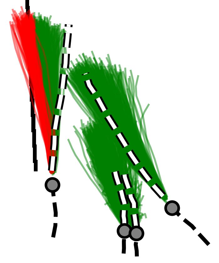
2       T. Salzmann? , B. Ivanovic? , P. Chakravarty, M. Pavone

Fig. 1. Exemplary road scene depicting pedestrians crossing a road in front of a vehicle
which may continue straight or turn right. The graph representation of the scene is
shown on the ground, where each agent and their interactions are represented as nodes
and edges, visualized as white circles and dashed black lines, respectively. Arrows depict
potential future agent velocities, with colors representing different high-level future
behavior modes.

    There are many existing methods for multi-agent behavior prediction, rang-
ing from deterministic regressors to generative, probabilistic models. However,
many of them were developed without directly accounting for real-world robotic
use cases; in particular, they ignore agents’ dynamics constraints, the ego-agent’s
own motion (important to capture the interactive aspect in human-robot inter-
action), and a plethora of environmental information (e.g., camera images, lidar,
maps) to which modern robotic systems have access. The few methods which do
include such considerations are closed-source, tightly integrated with a specific
robotic platform, or trained on private data [50,8,20,7].
    Accordingly, in this work we are interested in developing a multi-agent be-
havior prediction model that (1) accounts for the dynamics of the agents, and
in particular of ground vehicles [26,35]; (2) produces predictions possibly condi-
tioned on potential future robot trajectories, useful for intelligent planning tak-
ing into account human responses; and (3) provides a generally-applicable, open,
and extensible approach which can effectively use heterogeneous data about the
surrounding environment. Importantly, making use of such data would allow for
the incorporation of environmental information, e.g., maps, which would enable
producing predictions that differ depending on the structure of the scene (e.g.,
interactions at an urban intersection are very different from those in an open
sports field!). One method that comes close is the Trajectron [18], a multi-agent
behavior model which can handle a time-varying number of agents, accounts
for multimodality in human behavior (i.e., the potential for many high-level fu-
tures), and maintains a sense of interpretability in its outputs. However, the
Trajectron only reasons about relatively simple vehicle models (i.e., cascaded
integrators) and past trajectory data (i.e., no considerations are made for added
environmental information, if available).
    In this work we present Trajectron++, an open and extensible approach built
upon the Trajectron [18] framework which produces dynamically-feasible trajec-
tory forecasts from heterogeneous input data for multiple interacting agents of
distinct semantic types. Our key contributions are twofold: First, we show how
to effectively incorporate high-dimensional data through the lens of encoding
Trajectron++: Dynamically-Feasible Trajectory Forecasting 3
semantic maps. Second, we propose a general method of incorporating dynam-
ics constraints into learning-based methods for multi-agent trajectory forecast-
ing. Trajectron++ is designed to be tightly integrated with downstream robotic
modules, with the ability to produce trajectories that are optionally conditioned
on future ego-agent motion plans. We present experimental results on a vari-
ety of datasets, which collectively demonstrate that Trajectron++ outperforms
an extensive selection of state-of-the-art deterministic and generative trajectory
prediction methods, in some cases achieving 60% lower average prediction error.
2 Related Work
Deterministic Regressors. Many earlier works in human trajectory forecast-
ing were deterministic regression models. One of the earliest, the Social Forces
model [15], models humans as physical objects affected by Newtonian forces
(e.g., with attractors at goals and repulsors at other agents). Since then, many
approaches have been applied to the problem of trajectory forecasting, formu-
lating it as a time-series regression problem and applying methods like Gaussian
Process Regression (GPR) [38,47], Inverse Reinforcement Learning (IRL) [32],
and Recurrent Neural Networks (RNN) [1,33,46] to good effect. However, IRL
relies on a unimodal assumption of interaction outcome [25,34], making model-
ing multimodal data difficult. GPR falls prey to long inference times, whereas
robotic use cases necessitate fast inference, e.g., for frequent replanning. While
RNNs alone cannot model multimodality, they currently outperform all previous
deterministic regression models. As a result, they are commonly found as a core
component of human trajectory models [1,21,46].
Generative, Probabilistic Approaches. Recently, generative approaches
have emerged as state-of-the-art trajectory forecasting methods due to recent
advancements in deep generative models [43,12]. Notably, they have caused a
shift from focusing on predicting the single best trajectory to producing a dis-
tribution of potential future trajectories. This is advantageous in autonomous
systems as full distribution information is more useful for downstream tasks,
e.g., motion planning and decision making where information such as variance
can be used to make safer decisions. Most works in this category use a deep
recurrent backbone architecture with a latent variable model, such as a Condi-
tional Variational Autoencoder (CVAE) [43], to explicitly encode multimodality
[31,19,11,41,18,39], or a Generative Adversarial Network (GAN) [12] to implicitly
do so [13,40,27]. Common to both approach styles is the need to produce position
distributions. GAN-based models can directly produce these and CVAE-based
recurrent models usually rely on a bivariate Gaussian Mixture Model (GMM)
to output position distributions. However, both of these output structures make
it difficult to enforce dynamics constraints, e.g., non-holonomic constraints such
as those arising from no side-slip conditions.
Of these, the Trajectron [18] and Social-BiGAT [27] are the best-performing
CVAE-based and GAN-based models, respectively, on standard trajectory fore-
casting benchmarks [37,30]. They both present strong frameworks that address
many of our desiderata, however, they crucially do not account for dynamics
models or heterogeneous input data and lack experimental validation in the4 T. Salzmann? , B. Ivanovic? , P. Chakravarty, M. Pavone
presence of multiple semantic classes of agents (their experimental suites only
contain pedestrians as agents).
Currently, these deterministic and generative lines of work are disparate in
that models are solely designed to either produce one trajectory or a distribution
of trajectories. A generally-applicable approach should be able to produce either
output structure depending on the desired use case. While probabilistic models
may produce these intrinsically (e.g., predicting the mean or mode), questions
arise regarding multimodal distributions (which mode is “best”) and if the mean
corresponds to feasible trajectories. Further, many recent methods are GAN-
based and thus unable to obtain any distributional information beyond sampling.
Accounting for Dynamics and Heterogeneous Data. There are few
works that account for dynamics or make use of data modalities outside of prior
trajectory information. This is mainly because standard trajectory forecasting
benchmarks seldom include any other information, a fact that will surely change
following the recent release of autonomous vehicle-based datasets with rich multi-
sensor data [49,6,9,24]. The few works that do incorporate additional data pro-
duce trajectory forecasts from raw point clouds, High-Definition (HD) semantic
maps, and their histories, all showing performance improvements over previ-
ous approaches [50,8,20,7]. These approaches generally make use of end-to-end
learning architectures that encode raw sensor observations with Convolutional
Neural Networks (CNNs) and are trained to optimize multi-task objectives. A
downside of such architectures is that they can only operate on a fixed time his-
tory (CNN weights have fixed size), whereas recurrent architectures are able to
take into account all available historical information. Further, these approaches
are closed-source and trained on private datasets, making it virtually impos-
sible to reproduce or extend the proposed methods. As for dynamics, current
methods almost exclusively reason about positional information. This does not
capture dynamical constraints, however, which might lead to predictions in po-
sition space that are unrealizable by the underlying control variables (e.g., a car
moving sideways).
3 Problem Formulation
We aim to generate plausible trajectory distributions for a time-varying number
N (t) of interacting agents A1 , ..., AN (t) . Each agent Ai has a semantic class Si ,
e.g., Car, Bus, or Pedestrian. At time t, given the state s ∈ RD of each agent
and all of their histories for the previous H timesteps, which we denote as x,
(t−H:t)
x = s1,...,N (t) ∈ R(H+1)×N (t)×D , as well as additional information available to
(t)
each agent I1,...,N (t) , we seek a distribution over all agents’ future states for the
(t+1:t+T )
next T timesteps y = s1,...,N (t) ∈ RT ×N (t)×D , which we denote as p(y | x, I).
Unlike previous works where only an agent’s past and present position are
input, we wish to use more of the heterogeneous data that modern robotic sensor
suites provide. Specifically, for each agent i at time t we also assume that geomet-
(t)
ric semantic maps are available around Ai ’s position, Mi ∈ RdC/re×dC/re×L ,
with context size C × C, spatial resolution r, and L semantic channels. Depend-
ing on the dataset, these maps can range in sophistication from simple obstacleTrajectron++: Dynamically-Feasible Trajectory Forecasting 5
Node History Decoder
LSTM LSTM ŷ1(t+1) ŷ1(t+2)
x (t-1)
1
x (t)
1
∫ ∫
Edge
pθ(z|x,M,yR)
LSTM LSTM GMM GMM
F
x2,3
(t-1)
x2,3
(t)
A
T + e C
x
z
F
T GRU GRU
F C
LSTM LSTM
N + C
qϕ(z|x,y,M,yR) [ex,R;z;y(t)] [ex,R;z;ŷ(t+1)]
x4,R
(t-1)
x(t)
4,R
Map
CNN F
C
M
(t)
LEGEND
1
∫ Dynamics Integration
Robot Future
eR F
LSTM LSTM Dense Layer
C
x(t+(T-1)) xR(t+T) Random Sampling
R
+ Concatenation
Node Future ey Of f line Training
LSTM LSTM
Online Inference
x (t+(T-1))
x(t+T)
1 1
Both
Fig. 2. Left: Our approach represents a scene as a directed spatiotemporal graph.
Nodes and edges represent agents and their interactions, respectively. Right: The
corresponding network architecture for Node 1.
occupancy grids to multiple layers of human-annotated semantic information
(e.g., marking out sidewalks, road boundaries, and crosswalks).
One of our key desiderata is the ability to produce trajectories that take into
account ego-agent motion plans, for downstream use in motion planning, decision
making, and control. Thus, we also consider the setting where we condition on
an ego-agent’s future motion plan, for example when evaluating responses to a
set of motion primitives. In this setting, we additionally assume that we know
(t+1:t+T )
the ego-agent’s future motion plan for the next T timesteps, yR = sR .
4 Trajectron++
Our approach1 is visualized in Figure 2. At a high level, a spatiotemporal graph
representation of the scene in question is created from its topology. Then, a
similarly-structured deep learning architecture is generated that forecasts the
evolution of node attributes, producing agent trajectories.
Scene Representation. The current scene is abstracted as a spatiotemporal
graph G = (V, E). Nodes represent agents and edges represent their interactions.
As a result, in the rest of the paper we will use the terms “node” and “agent”
interchangeably. Each node also has a semantic class matching the class of its
agent (e.g., Car, Bus, Pedestrian). An edge (Ai , Aj ) is present in E if Ai influ-
ences Aj . In this work, the `2 distance is used as a proxy for whether agents
are influencing each other or not. Formally, an edge is directed from Ai to Aj if
kpi − pj k2 ≤ dSj where pi , pj ∈ R2 are the 2D world positions of agents Ai , Aj ,
respectively, and dSj is a distance that encodes the perception range of agents of
semantic class Sj . While more sophisticated methods can be used to construct
edges (e.g., [46]), they usually incur extra computational overhead by requiring
a complete scene graph. Figure 2 shows an example of this scene abstraction.
1
All of our source code, trained models, and data can be found online at
https://github.com/StanfordASL/Trajectron-plus-plus.6 T. Salzmann? , B. Ivanovic? , P. Chakravarty, M. Pavone
An important benefit of abstracting the original scene in this way is that
it enables our approach to be applied to various problem domains, provided
they can be modeled as spatiotemporal graphs. We specifically choose to model
the scene as a directed graph, in contrast to an undirected one as in previous
approaches [21,1,13,46,19,18], because a directed graph can represent a more
general set of scenes and interaction types, e.g., asymmetric influence. This pro-
vides the additional benefit of being able to simultaneously model agents with
different perception ranges, e.g., the driver of a car looks much farther ahead on
the road than a pedestrian does while walking on the sidewalk.
Modeling Agent History. Once a graph of the scene is constructed, the
model needs to encode a node’s current state, its history, and how it is influ-
enced by its neighboring nodes. To encode the observed history of the modeled
agent, their current and previous states are fed into a Long Short-Term Mem-
ory (LSTM) network [17] with 32 hidden dimensions. Since we are interested in
(t−H:t)
modeling trajectories, the inputs x = s1,...,N (t) ∈ R(H+1)×N (t)×D are the current
and previous D-dimensional states of the modeled agents. These are typically
positions and velocities, which can be easily estimated online.
Ideally, agent models should be chosen to best match their semantic class
Si . For example, one would usually model vehicles on the road using a bicycle
model [26,35]. However, estimating the bicycle model parameters of another ve-
hicle from online observations is very difficult as it requires estimation of the
vehicle’s center of mass, wheelbase, and front wheel steer angle. As a result, in
this work pedestrians are modeled as single integrators and wheeled vehicles are
modeled as dynamically-extended unicycles [28], enabling us to account for key
non-holonomic constraints (e.g., no side-slip constraints) [35] without requiring
complex online parameter estimation procedures – we will show through exper-
iments that such a simplified model is already quite impactful on improving
prediction accuracy. While the dynamically-extended unicycle model serves as
an important representative example, we note that our approach can also be
generalized to other dynamics models, provided its parameters can either be
assumed or quickly estimated online.
Encoding Agent Interactions. To model neighboring agents’ influence on
the modeled agent, Trajectron++ encodes graph edges in two steps. First, edge
information is aggregated from neighboring agents of the same semantic class. In
this work, an element-wise sum is used as the aggregation operation. We choose
to combine features in this way rather than with concatenation or an average to
handle a variable number of neighboring nodes with a fixed architecture while
preserving count information [3,19,21]. These aggregated states are then fed into
an LSTM with 8 hidden dimensions whose weights are shared across all edge in-
stances of the same type, e.g., all Pedestrian-Bus edge LSTMs share the same
weights. Then, the encodings from all edge types that connect to the modeled
node are aggregated to obtain one “influence” representation vector, represent-
ing the effect that all neighboring nodes have. For this, an additive attention
module is used [2]. Finally, the node history and edge influence encodings are
concatenated to produce a single node representation vector, ex .
Incorporating Heterogeneous Data. Modern sensor suites are able to
produce much more information than just tracked trajectories of other agents.
Notably, HD maps are used by many real-world systems to aid localization as wellTrajectron++: Dynamically-Feasible Trajectory Forecasting 7
as inform navigation. Depending on sensor availability and sophistication, maps
can range in fidelity from simple binary obstacle maps, i.e., M ∈ {0, 1}H×W ×1 ,
to HD semantic maps, e.g., M ∈ {0, 1}H×W ×L where each layer 1 ≤ ` ≤ L
corresponds to an area with semantic type (e.g., “driveable area,” “road block,”
“walkway,” “pedestrian crossing”). To make use of this information, for each
modeled agent, Trajectron++ encodes a local map, rotated to match the agent’s
heading, with a CNN. The CNN has 4 layers, with filters {5, 5, 5, 3} and respec-
tive strides of {2, 2, 1, 1}. These are followed by a dense layer with 32 hidden
dimensions, the output of which is concatenated with the node history and edge
influence representation vectors.
More generally, one can include further additional information (e.g., raw
LIDAR data, camera images, pedestrian skeleton or gaze direction estimates)
in this framework by encoding it as a vector and adding it to this backbone of
representation vectors, ex .
Encoding Future Ego-Agent Motion Plans. Producing predictions which
take into account future ego-agent motion is an important capability for robotic
decision making and control. Specifically, it allows for the evaluation of a set
of motion primitives with respect to possible responses from other agents. Tra-
jectron++ can encode the future T timesteps of the ego-agent’s motion plan
yR using a bi-directional LSTM with 32 hidden dimensions. A bi-directional
LSTM is used due to its strong performance on other sequence summarization
tasks [5]. The final hidden states are then concatenated into the backbone of
representation vectors, ex .
Explicitly Accounting for Multimodality. Trajectron++ explicitly han-
dles multimodality by leveraging the CVAE latent variable framework [43]. It
produces the target p(y | x) distribution by introducing a discrete Categorical
latent variable z ∈ Z which encodes high-level latent behavior and allows for
p(y | x) to be expressed as X
p(y | x) = pψ (y | x, z)pθ (z | x), (1)
z∈Z
where |Z| = 25 and ψ, θ are deep neural network weights that parameterize their
respective distributions. z being discrete also aids in interpretability, as one can
visualize which high-level behaviors belong to each z by sampling trajectories.
During training, a bi-directional LSTM with 32 hidden dimensions is used to
encode a nodes ground truth future trajectory, producing qφ (z | x, y) [43].
Producing Dynamically-Feasible Trajectories. After obtaining a la-
tent variable z, it and the backbone representation vector ex are fed into the
decoder, a 128-dimensional Gated Recurrent Unit (GRU) [10]. Each GRU cell
outputs the parameters of a bivariate Gaussian distribution over control ac-
tions u(t) (e.g., acceleration and steering rate). The agent’s system dynamics
are then integrated with the produced control actions u(t) to obtain trajectories
in position space [23,45]. The only uncertainty at prediction time stems from
Trajectron++’s output. Thus, in the case of linear dynamics (e.g., single inte-
grators, used in this work to model pedestrians), the system dynamics are linear
Gaussian. Explicitly, for a single integrator with control actions u(t) = ṗ(t) ,
(t+1) (t) (t) (t)
the position mean at t + 1 is µp = µp + µu ∆t, where µu is produced by
Trajectron++. In the case of nonlinear dynamics (e.g., unicycle models, used in
this work to model vehicles), one can still (approximately) use this uncertainty8 T. Salzmann? , B. Ivanovic? , P. Chakravarty, M. Pavone
propagation scheme by linearizing the dynamics about the agent’s current state
and control. Full mean and covariance equations for the single integrator and
dynamically-extended unicycle models are in the appendix. In contrast to exist-
ing methods which directly output positions, our approach is uniquely able to
guarantee that its trajectory samples are dynamically feasible by integrating an
agent’s dynamics with the predicted controls.
Output Configurations. Based on the desired use case, Trajectron++ can
produce many different outputs. The main four are outlined below.
1. Most Likely (ML): The model’s deterministic and most-likely single output.
The high-level latent behavior mode and output trajectory are the modes of
their respective distributions, where
zmode = arg max pθ (z | x), y = arg max pψ (y | x, zmode ). (2)
z y
2. zmode : Predictions from the model’s most-likely high-level latent behavior
mode, where
zmode = arg max pθ (z | x), y ∼ pψ (y | x, zmode ). (3)
z
3. Full : The model’s full sampled output, where z and y are sampled sequen-
tially according to
z ∼ pθ (z | x), y ∼ pψ (y | x, z). (4)
4. Distribution: Due to the use of a discrete latent variable and Gaussian output
structure, the model can provide an analytic output distribution by directly
computing Equation (1).
Training the Model. We adopt the InfoVAE [51] objective function, and
modify it to use discrete latent states in a conditional formulation (since the
model uses a CVAE). Formally, we aim to solve
XN
max Ez∼qφ (·|xi ,yi ) log pψ (yi | xi , z)
φ,θ,ψ
i=1
(5)
− βDKL qφ (z | xi , yi ) k pθ (z | xi )
+ αIq (x; z),
where Iq is the mutual information between x and z under the distribution
qφ (x, z). To compute Iq , we follow [51] and approximate qφ (z | xi , yi ) with
pθ (z | xi ), obtaining the unconditioned latent distribution by summing out xi
over the batch. Notably, the Gumbel-Softmax reparameterization [22] is not
used to backpropagate through the Categorical latent variable z because it is
not sampled during training time. Instead, the first term of Equation (5) is
directly computed since the latent space has only |Z| = 25 discrete elements. A
discussion on choosing α and β can be found in the appendix.
To avoid overfitting to environment-specific characteristics, such as the gen-
eral directions that agents move, we augment the data from each scene. We
rotate all trajectories in a scene around the scene’s origin by γ, where γ varies
from 0◦ to 360◦ (exclusive) in 15◦ intervals. The benefits of dataset augmentation
by trajectory rotation have already been studied for pedestrians [42]. We apply
this same augmentation to autonomous driving datasets as most of them are
recorded in cities whose streets are roughly orthogonal and separated by blocks.
Additional training information can be found in the appendix.Trajectron++: Dynamically-Feasible Trajectory Forecasting 9
5 Experiments
Our method is evaluated on three publicly-available datasets: The ETH [37],
UCY [30], and nuScenes [6] datasets. The ETH and UCY datasets consist of real
pedestrian trajectories with rich multi-human interaction scenarios captured at
2.5 Hz (∆t = 0.4s). In total, there are 5 sets of data, 4 unique scenes, and 1536
unique pedestrians. They are a standard benchmark in the field, containing chal-
lenging behaviors such as couples walking together, groups crossing each other,
and groups forming and dispersing. However, they only contain pedestrians, so
we also evaluate on the recently-released nuScenes dataset. It is a large-scale
dataset for autonomous driving with 1000 scenes in Boston and Singapore. Each
scene is annotated at 2 Hz (∆t = 0.5s) and is 20s long, containing up to 23
semantic object classes as well as HD semantic maps with 11 annotated layers.
Trajectron++ was implemented in PyTorch [36] on a desktop computer run-
ning Ubuntu 18.04 containing an AMD Ryzen 1800X CPU and two NVIDIA
GTX 1080 Ti GPUs. We trained the model for 100 epochs (∼ 3 hours) on the
pedestrian datasets and 12 epochs (∼ 8 hours) on the nuScenes dataset.
Evaluation Metrics. As in prior work [1,13,18,40,27], our method for tra-
jectory forecasting is evaluated with the four following error metrics:
1. Average Displacement Error (ADE): Mean `2 distance between the ground
truth and predicted trajectories.
2. Final Displacement Error (FDE): `2 distance between the predicted final
position and the ground truth final position at the prediction horizon T .
3. Kernel Density Estimate-based Negative Log Likelihood (KDE NLL): Mean
NLL of the ground truth trajectory under a distribution created by fitting a
kernel density estimate on trajectory samples [18,44].
4. Best-of-N (BoN): The minimum ADE and FDE from N randomly-sampled
trajectories.
We compare our method to an exhaustive set of state-of-the art deterministic
and generative approaches.
Deterministic Baselines. Our method is compared against the following
deterministic baselines: (1) Linear : A linear regressor with parameters estimated
by minimizing least square error. (2) LSTM : An LSTM network with only agent
history information. (3) Social LSTM [1]: Each agent is modeled with an LSTM
and nearby agents’ hidden states are pooled at each timestep using a proposed
social pooling operation. (4) Social Attention [46]: Same as [1], but all other
agents’ hidden states are incorporated via a proposed social attention operation.
Generative Baselines. On the ETH and UCY datasets, our method is com-
pared against the following generative baselines: (1) S-GAN [13]: Each agent is
modeled with an LSTM-GAN, which is an LSTM encoder-decoder whose out-
puts are the generator of a GAN. The generated trajectories are then evaluated
against the ground truth trajectories with a discriminator. (2) S-GAN-P [13]:
Same as S-GAN, but including their proposed global pooling scheme. (3) So-
Phie [40]: An LSTM-GAN with the addition of a proposed physical and social
attention module. (4) Social-BiGAT [27]: An LSTM-GAN with the addition of
a Graph Attention Network (GAT) to encode agent relationships. (5) Trajec-
tron [18]: An LSTM-CVAE encoder-decoder which is explicitly constructed to10 T. Salzmann? , B. Ivanovic? , P. Chakravarty, M. Pavone
Table 1. (a) Our model’s deterministic Most Likely output outperforms other deter-
ministic methods on displacement error metrics, even if it was not originally trained to
do so. (b) Our model’s probabilistic Full output significantly outperforms other meth-
ods, yielding accurate predictions even in a small number of samples. Lower is better.
Bold indicates best.
Dataset (a) ADE/FDE (m)
R
Linear LSTM S-LSTM [13] S-ATTN [46] Ours (ML) Ours+ (ML)
ETH 1.33/2.94 1.09/2.41 1.09/2.35 0.39/3.74 0.71/1.66 0.71/1.68
Hotel 0.39/0.72 0.86/1.91 0.79/1.76 0.29/2.64 0.22/0.46 0.22/0.46
Univ 0.82/1.59 0.61/1.31 0.67/1.40 0.33/3.92 0.44/1.17 0.41/1.07
Zara 1 0.62/1.21 0.41/0.88 0.47/1.00 0.20/0.52 0.30/0.79 0.30/0.77
Zara 2 0.77/1.48 0.52/1.11 0.56/1.17 0.30/2.13 0.23/0.59 0.23/0.59
Average 0.79/1.59 0.70/1.52 0.72/1.54 0.30/2.59 0.39/1.02 0.37/0.95
Dataset (b) ADE/FDE, Best of 20 Samples (m)
R
S-GAN [13] SoPhie [40] Trajectron [18] S-BiGAT [27] Ours (Full) Ours+ (Full)
ETH 0.81/1.52 0.70/1.43 0.59/1.14 0.69/1.29 0.39/0.83 0.43/0.86
Hotel 0.72/1.61 0.76/1.67 0.35/0.66 0.49/1.01 0.12/0.21 0.12/0.19
Univ 0.60/1.26 0.54/1.24 0.54/1.13 0.55/1.32 0.20/0.44 0.22/0.43
Zara 1 0.34/0.69 0.30/0.63 0.43/0.83 0.30/0.62 0.15/0.33 0.17/0.32
Zara 2 0.42/0.84 0.38/0.78 0.43/0.85 0.36/0.75 0.11/0.25 0.12/0.25
Average 0.58/1.18 0.54/1.15 0.56/1.14 0.48/1.00 0.18/0.40 0.20/0.39
R
Legend: = Integration via Dynamics, M = Map Encoding, yR = Robot Future Encoding
match the spatiotemporal structure of the scene. Its scene abstraction is similar
to ours, but uses undirected edges.
On the nuScenes dataset, the following methods are also compared against:
(6) Convolutional Social Pooling (CSP) [11]: An LSTM-based approach which
explicitly considers a fixed number of movement classes and predicts which of
those the modeled agent is likely to take. (7) CAR-Net [41]: An LSTM-based
approach which encodes scene context with visual attention. (8) SpAGNN [7]: A
CNN encodes raw LIDAR and semantic map data to produce object detections,
from which a Graph Neural Network (GNN) produces probabilistic, interaction-
aware trajectories.
Evaluation Methodology. For the ETH and UCY datasets, a leave-one-out
strategy is used for evaluation, similar to previous works [1,13,18,27,40], where
the model is trained on four datasets and evaluated on the held-out fifth. An
observation length of 8 timesteps (3.2s) and a prediction horizon of 12 timesteps
(4.8s) is used for evaluation. For the nuScenes dataset, there are explicit train,
validation, and test splits. However, the ground truth test annotations are not
public. Instead, we split off 15% of the train set for hyperparameter tuning and
test on the provided validation set.
Throughout the following, we report the performance of Trajectron++ in
multiple configurations. Specifically, Ours refers to the base model using only
node and edge encoding, trained to predict
R agent velocities and Euler integrating
velocity to produce positions; Ours+ is the base model with dynamics inte-
gration, trained to predict control actions and integrating
R the agent’s dynamics
with the control actions to produce positions;
R Ours+ , M additionally includes
the map encoding CNN; and Ours+ , M, yR adds the robot future encoder.Trajectron++: Dynamically-Feasible Trajectory Forecasting 11
Table 2. Mean KDE-based NLL for each dataset. Lower is better. 2000 trajectories
were sampled per model at each prediction timestep. Bold indicates the best values.
Dataset KDE NLL
R
S-GAN [13] Trajectron [18] Ours (Full) Ours+ (Full)
ETH 15.70 2.99 1.80 1.31
Hotel 8.10 2.26 −1.29 −1.94
Univ 2.88 1.05 −0.89 −1.13
Zara 1 1.36 1.86 −1.13 −1.41
Zara 2 0.96 0.81 −2.19 −2.53
Average 3.68 1.30 −1.12 −1.39
R
Legend: = Integration via Dynamics, M = Map Encoding, yR = Robot Future Encoding
5.1 ETH and UCY Datasets
Our approach is first evaluated on the ETH [37] and UCY [30] Pedestrian
Datasets, against deterministic methods on standard trajectory forecasting met-
rics. It is difficult to determine the current state-of-the-art in deterministic meth-
ods as there are contradictions between the results reported by the same authors
in [13] and [1]. In Table 1 of [1], Social LSTM convincingly outperforms a base-
line LSTM without pooling. However, in Table 1 of [13], Social LSTM is actually
worse than the same baseline on average. Thus, when comparing against Social
LSTM we report the results summarized in Table 1 of [13] as it is the most re-
cent work by the same authors. Further, the values reported by Social Attention
in [46] seem to have unusually high ratios of FDE to ADE. Nearly every other
method (including ours) has FDE/ADE ratios around 2 − 3× whereas Social At-
tention’s are around 3 − 12×. Social Attention’s errors on the Univ dataset are
especially striking, as its FDE of 3.92 is 12× its ADE of 0.33, meaning its predic-
tion error on the other 11 timesteps is essentially zero. We still compare against
the values reported in [46] as there is no publicly-released code, but this raises
doubts of their validity. To fairly compare against prior work, neither map en-
coding nor future motion plan encoding is used. Only the node history and edge
encoders are used in the model’s encoder. Additionally, the model’s deterministic
ML output scheme is employed, which produces the model’s most likely single
trajectory. Table 1 (a) summarizes these results and shows that our approach is
competitive with state-of-the-art deterministic regressors on displacement error
metrics (outperforming existing approaches by 33% on mean FDE), even though
our method was not originally trained to minimize this. It makes sense that the
model performs similarly with and without dynamics integration for pedestri-
ans, since they are modeled as single integrators. Thus, their control actions are
velocities which matches the base model’s output structure.
To more concretely compare generative methods, we use the KDE-based
NLL metric proposed in [18,44], an approach that maintains full output dis-
tributions and compares the log-likelihood of the ground truth under different
methods’ outputs. Table 2 summarizes these results and shows that our method
significantly outperforms others. This is also where the performance improve-
ments brought by the dynamics integration scheme are clear. It yields the best
performance because the model is now explicitly trained on the distribution
it is seeking to output (the loss function term pψ (y|x, z) is now directly over
positions), whereas the base model is trained on velocity distributions, the in-
tegration of which (with no accounting for system dynamics) introduces errors.12 T. Salzmann? , B. Ivanovic? , P. Chakravarty, M. Pavone
Fig. 3. [ETH] Left: When only using trajectory data, Trajectron++ does not know
of obstacles and makes predictions into walls (in red). Right: Encoding a local map
of the agent’s surroundings significantly reduces the frequency of obstacle-violating
predictions.
Table 3. [nuScenes] (a): Vehicle-only FDE across time for Trajectron++ compared
to that of other single-trajectory and probabilistic approaches. Bold indicates best.
(b): Pedestrian-only FDE and KDE NLL across time for Trajectron++.
(a) Vehicle-only
FDE (m)
Method
@1s @2s @3s @4s (b) Pedestrian-only
Const. Velocity 0.32 0.89 1.70 2.73 KDE NLL FDE (m)
Method
S-LSTM∗ [1,7] 0.47 - 1.61 - @1s @2s @3s @4s @1s @2s @3s @4s
CSP∗ [11,7] 0.46 - 1.50 -
CAR-Net∗ [41,7] 0.38 - 1.35 - Ours (ML) −2.69 −2.46 −1.76 −1.09 0.03 0.17 0.37 0.60
SpAGNN∗ [7]
R
0.36 - 1.23 - Ours+ ,M (ML) −5.58 −3.96 −2.77 −1.89 0.01 0.17 0.37 0.62
Ours (ML)
R 0.18 0.57 1.25 2.24
Ours+ ,M (ML) 0.07 0.45 1.14 2.20
∗
We subtracted 22-24cm from these reported values (their detection/tracking error [7]), as we do
R not use a detector/tracker. This is done to establish a fair comparison.
Legend: = Integration via Dynamics, M = Map Encoding, yR = Robot Future Encoding.
Unfortunately, at this time there is no publicly-released code for SoPhie [40]
or Social-BiGAT [27], so they cannot be evaluated with the KDE-based NLL
metric. Instead, we evaluate Trajectron++ with the Best-of-N metric used in
their works. Table 1 (b) summarizes these results, and shows that our method
significantly improves over the previous state-of-the-art [27], achieving 55 − 60%
lower average errors.
Map Encoding. To evaluate the effect of incorporating heterogeneous data,
we compare the performance of Trajectron++ with and without the map encoder.
Specifically, we compare the frequency of obstacle violations in 2000 trajectory
samples from the Full model output on the ETH - University scene, which pro-
vides a simple binary obstacle map. Overall, our approach generates colliding
predictions 1.0% of the time with map encoding, compared to 4.6% without map
encoding. We also study how much of a reduction there is for pedestrians that
are especially close to an obstacle (i.e. they have at least one obstacle-violating
trajectory in their Full output), an example of which is shown in Figure 3. In
this regime, our approach generates colliding predictions 4.9% of the time with
map encoding, compared to 21.5% without map encoding.
5.2 nuScenes Dataset
To further evaluate the model’s ability to use heterogeneous data and simultane-
ously model multiple semantic classes of agents, we evaluate it on the nuScenes
dataset [6]. Again, the deterministic ML output scheme is used to fairly compareTrajectron++: Dynamically-Feasible Trajectory Forecasting 13
Table 4. [nuScenes] (a): Vehicle-only prediction performance for ablated versions of
our model. (b): The same, but excluding the ego-robot from consideration (as it is being
conditioned on). This shows that our model’s robot future conditional performance does
not arise from merely removing the ego-vehicle.
(a) Including the Ego-Vehicle
Ablation
R KDE NLL FDE ML (m) B. Viol. (%)
M yR @1s @2s @3s @4s @1s @2s @3s @4s @1s @2s @3s @4s
- - - 0.81 0.05 0.37 0.87 0.18 0.57 1.25 2.24 0.2 0.6 2.8 6.9
X - - −4.28 −2.82 −1.67 −0.76 0.07 0.45 1.13 2.17 0.2 0.7 3.2 8.1
X X - −4.17 −2.74 −1.62 −0.70 0.07 0.45 1.14 2.20 0.3 0.6 2.8 7.6
(b) Excluding the Ego-Vehicle
Ablation
R KDE NLL FDE ML (m) B. Viol. (%)
M yR @1s @2s @3s @4s @1s @2s @3s @4s @1s @2s @3s @4s
X X - −4.26 −2.86 −1.76 −0.87 0.07 0.44 1.09 2.09 0.3 0.6 2.8 7.6
X X X −3.90 −2.76 −1.75 −0.93 0.08 0.34 0.81 1.50 0.3 0.5 1.6 4.2
R
Legend: = Integration via Dynamics, M = Map Encoding, yR = Robot Future Encoding
with other single-trajectory predictors. The trajectories of both Pedestrians and
Cars are forecasted, two semantic object classes which account for most of the 23
possible object classes present in the dataset. To obtain an estimate of prediction
quality degradation over time, we compute the model’s FDE at t = {1, 2, 3, 4}s
for all tracked objects with at least 4s of available future data. We also imple-
ment a constant velocity baseline, which simply maintains the agent’s heading
and speed for the prediction horizon. Table 3 (a) summarizes the model’s perfor-
mance in comparison with state-of-the-art vehicle trajectory prediction models.
Since other methods use a detection/tracking module (whereas ours does not),
to establish a fair comparison we subtracted other methods’ detection and track-
ing error from their reported values. The dynamics integration scheme and map
encoding yield a noticeable improvement with vehicles, as their dynamically-
extended unicycle dynamics now differ from the single integrator assumption
made by the base model. Note that our method was only trained to predict 3s
into the future, thus its performance at 4s also provides a measure of its ca-
pability to generalize beyond its training configuration. Other methods do not
report values at 2s and 4s. As can be seen, Trajectron++ outperforms existing
approaches without facing a sharp degradation in performance after 3s. Our
approach’s performance on pedestrians is reported in Table 3 (b), where the
inclusion of HD maps and dynamics integration similarly improve performance
as in the pedestrian datasets.
Ablation Study. To develop an understanding of which model components
influence performance, a comprehensive ablation study is performed in Table 4.
As can be seen in the first row, even the base model’s deterministic ML output
performs strongly relative to current state-of-the-art approaches for vehicle tra-
jectory forecasting [7]. Adding the dynamics integration scheme yields a drastic
reduction in NLL as well as FDE at all prediction horizons. There is also an as-
sociated slight increase in the frequency of road boundary-violating predictions.
This is a consequence of training in position (as opposed to velocity) space, which
yields more variability in the corresponding predictions. Additionally including
map encoding maintains prediction accuracy while reducing the frequency of
boundary-violating predictions.14 T. Salzmann? , B. Ivanovic? , P. Chakravarty, M. Pavone
road_divider
lane_divider
Ours (ML)
Ground Truth
drivable_area
road_segment
lane
ped_crossing
walkway
stop_line
R R
(a) Ours (b)+ (c)+ , M
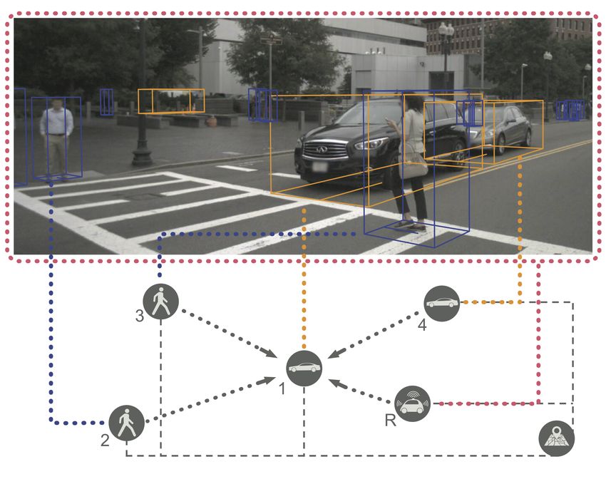
Fig. 4. [nuScenes] The same scene as forecast by three versions of Trajectron++.
(a) The base model tends to under-shoot turns, and makes overly-confident predictions.
(b) Our approach better captures position uncertainty with dynamics integration,
producing well-calibrated probabilities. (c) The model is able to leverage the additional
information that a map provides, yielding accurate predictions.
The effect of conditioning on the ego-vehicle’s future motion plan is also
studied, with results summarized in Table 4 (b). Conditioning on the ego-agent
removes its data from evaluation (excluding ∼ 15% of test data), so to compare
to the model with dynamics integration and map encoding from Table 4 (a) we
re-evaluate it with the ego-vehicle excluded. As one would expect, providing the
model with future motion plans of the ego-vehicle yields significant reductions
in error and road boundary violations. This use-case is common throughout au-
tonomous driving as the ego-vehicle repeatedly produces future motion plans at
every timestep by evaluating motion primitives. Overall, dynamics integration is
the dominant performance-improving module, making predictions more accurate
and feasible.
Qualitative Comparison. Figure 4 shows trajectory predictions from the
base model, with dynamics integration, and with dynamics integration + map
encoding. In it, one can see that the base model (predicting in velocity space)
undershoots the turn for the red car, predicting that it will end up in oncom-
ing traffic. Worse, the base model is overconfident, producing tight distributions
that do not coincide with the ground truth. With the integration of dynamics,
the model captures multimodality in the agent’s action, predicting both the pos-
sibility of a right turn and continuing straight. While this is more accurate than
the base model, there is still probability mass extending across lane boundaries.
With the addition of map encoding, the predictions are not only more accurate,
but nearly all probability mass now lies within the correct side of the road. This
is in contrast to versions of the model without map encoding which predict that
the red car might move into oncoming traffic.
6 Conclusion
In this work, we present Trajectron++, a generative multi-agent trajectory fore-
casting approach which uniquely addresses our desiderata for an open, generally-
applicable, and extensible framework. It can incorporate heterogeneous data
beyond prior trajectory information and is able to produce future-conditional
predictions that respect dynamics constraints, all while producing full probabil-
ity distributions, which are especially useful in downstream robotic tasks such
as motion planning, decision making, and control. It achieves state-of-the-art
prediction performance in a variety of metrics on standard and new real-world
multi-agent human behavior datasets.Trajectron++: Dynamically-Feasible Trajectory Forecasting 15
Future directions include incorporating human behavior predictions from
Trajectron++ in robotic motion planning, decision making, and control frame-
works, each of which are core tasks that are solved online by autonomous systems.
Another key future direction is using Trajectron++ in simulation, generating re-
alistic human trajectories in simulated environments. Finally, there is still a
whole host of heterogeneous data that can be incorporated into this model, e.g.,
raw LIDAR data, raw camera images, 2D/3D semantic segmentation. which are
left as future work.
Acknowledgment. Tim Salzmann is supported by a fellowship within the
IFI programme of the German Academic Exchange Service (DAAD). We thank
Matteo Zallio for his help in visually communicating our work and Amine Elhafsi
for sharing his dynamics knowledge and proofreading. We also thank Brian Yao
for improving our pedestrian dataset evaluation script. This work was supported
in part by the Ford-Stanford Alliance. This article solely reflects the opinions
and conclusions of its authors.16 T. Salzmann? , B. Ivanovic? , P. Chakravarty, M. Pavone
References
1. Alahi, A., Goel, K., Ramanathan, V., Robicquet, A., Fei-Fei, L., Savarese, S.:
Social LSTM: Human trajectory prediction in crowded spaces. In: IEEE Conf. on
Computer Vision and Pattern Recognition (2016) 3, 6, 9, 10, 11, 12
2. Bahdanau, D., Cho, K., Bengio, Y.: Neural machine translation by jointly learning
to align and translate. In: Int. Conf. on Learning Representations (2015) 6
3. Battaglia, P.W., Pascanu, R., Lai, M., Rezende, D., Kavukcuoglu, K.: Interaction
networks for learning about objects, relations and physics. In: Conf. on Neural
Information Processing Systems (2016) 6
4. Bowman, S.R., Vilnis, L., Vinyals, O., Dai, A.M., Jozefowicz, R., Bengio, S.: Gen-
erating sentences from a continuous space. In: Proc. Annual Meeting of the Asso-
ciation for Computational Linguistics (2015) 22
5. Britz, D., Goldie, A., Luong, M.T., Le, Q.V.: Massive exploration of neural ma-
chine translation architectures. In: Proc. of Conf. on Empirical Methods in Natural
Language Processing. pp. 1442–1451 (2017) 7
6. Caesar, H., Bankiti, V., Lang, A.H., Vora, S., Liong, V.E., Xu, Q., Krishnan, A.,
Pan, Y., Baldan, G., Beijbom, O.: nuScenes: A multimodal dataset for autonomous
driving (2019) 4, 9, 12
7. Casas, S., Gulino, C., Liao, R., Urtasun, R.: SpAGNN: Spatially-aware graph neu-
ral networks for relational behavior forecasting from sensor data (2019) 2, 4, 10,
12, 13
8. Casas, S., Luo, W., Urtasun, R.: IntentNet: Learning to predict intention from raw
sensor data. In: Conf. on Robot Learning. pp. 947–956 (2018) 2, 4
9. Chang, M.F., Lambert, J., Sangkloy, P., Singh, J., Bak, S., Hartnett, A., Wang, D.,
Carr, P., Lucey, S., Ramanan, D., Hays, J.: Argoverse: 3d tracking and forecasting
with rich maps. In: IEEE Conf. on Computer Vision and Pattern Recognition
(2019) 4
10. Cho, K., van Merrienboer, B., Gulcehre, C., Bahdanau, D., Bougares, F., Schwenk,
H., Bengio, Y.: Learning phrase representations using rnn encoder-decoder for
statistical machine translation. In: Proc. of Conf. on Empirical Methods in Natural
Language Processing. pp. 1724–1734 (2014) 7
11. Deo, M.F., Trivedi, J.: Multi-modal trajectory prediction of surrounding vehicles
with maneuver based lstms. In: IEEE Intelligent Vehicles Symposium (2018) 3,
10, 12
12. Goodfellow, I., Pouget-Abadie, J., Mirza, M., Xu, B., Warde-Farley, D., Ozair,
S., Courville, A., Bengio, Y.: Generative adversarial nets. In: Conf. on Neural
Information Processing Systems (2014) 3
13. Gupta, A., Johnson, J., Fei-Fei, L., Savarese, S., Alahi, A.: Social GAN: Socially
acceptable trajectories with generative adversarial networks. In: IEEE Conf. on
Computer Vision and Pattern Recognition (2018) 3, 6, 9, 10, 11
14. Gweon, H., Saxe, R.: Developmental cognitive neuroscience of theory of mind. In:
Neural Circuit Development and Function in the Brain, chap. 20. Academic Press
(2013) 1
15. Helbing, D., Molnár, P.: Social force model for pedestrian dynamics. Physical Re-
view E 51(5), 4282–4286 (1995) 3
16. Higgins, I., Matthey, L., Pal, A., Burgess, C., Glorot, X., Botvinick, M., Mohamed,
S., Lerchner, A.: beta-VAE: Learning basic visual concepts with a constrained
variational framework. In: Int. Conf. on Learning Representations (2017) 22
17. Hochreiter, S., Schmidhuber, J.: Long short-term memory. Neural Computation
(1997) 6
18. Ivanovic, B., Pavone, M.: The Trajectron: Probabilistic multi-agent trajectory
modeling with dynamic spatiotemporal graphs. In: IEEE Int. Conf. on Computer
Vision. pp. 2375–2384 (2019) 2, 3, 6, 9, 10, 11, 21Trajectron++: Dynamically-Feasible Trajectory Forecasting 17
19. Ivanovic, B., Schmerling, E., Leung, K., Pavone, M.: Generative modeling of mul-
timodal multi-human behavior. In: IEEE/RSJ Int. Conf. on Intelligent Robots &
Systems (2018) 3, 6
20. Jain, A., Casas, S., Liao, R., Xiong, Y., Feng, S., Segal, S., Urtasun, R.: Discrete
residual flow for probabilistic pedestrian behavior prediction. In: Conf. on Robot
Learning (2019) 2, 4
21. Jain, A., Zamir, A.R., Savarese, S., Saxena, A.: Structural-RNN: Deep learning on
spatio-temporal graphs. In: IEEE Conf. on Computer Vision and Pattern Recog-
nition (2016) 3, 6
22. Jang, E., Gu, S., Poole, B.: Categorial reparameterization with gumbel-softmax.
In: Int. Conf. on Learning Representations (2017) 8
23. Kalman, R.E.: A new approach to linear filtering and prediction problems. ASME
Journal of Basic Engineering 82, 35–45 (1960) 7, 19
24. Kesten, R., Usman, M., Houston, J., Pandya, T., Nadhamuni, K., Ferreira, A.,
Yuan, M., Low, B., Jain, A., Ondruska, P., Omari, S., Shah, S., Kulkarni, A.,
Kazakova, A., Tao, C., Platinsky, L., Jiang, W., Shet, V.: Lyft Level 5 AV Dataset
2019. https://level5.lyft.com/dataset/ (2019) 4
25. Kober, J., Bagnell, J.A., Peters, J.: Reinforcement learning in robotics: A survey.
Int. Journal of Robotics Research 32(11), 1238 – 1274 (2013) 3
26. Kong, J., Pfeifer, M., Schildbach, G., Borrelli, F.: Kinematic and dynamic vehi-
cle models for autonomous driving control design. In: IEEE Intelligent Vehicles
Symposium (2015) 2, 6
27. Kosaraju, V., Sadeghian, A., Martı́n-Martı́n, R., Reid, I., Rezatofighi, S.H.,
Savarese, S.: Social-BiGAT: Multimodal trajectory forecasting using bicycle-GAN
and graph attention networks. In: Conf. on Neural Information Processing Systems
(2019) 3, 9, 10, 12
28. LaValle, S.M.: Better unicycle models. In: Planning Algorithms, pp. 743–743. Cam-
bridge Univ. Press (2006) 6, 19
29. LaValle, S.M.: A simple unicycle. In: Planning Algorithms, pp. 729–730. Cambridge
Univ. Press (2006) 19
30. Leal-Taixé, L., Fenzi, M., Kuznetsova, A., Rosenhahn, B., Savarese, S.: Learning
an image-based motion context for multiple people tracking. In: IEEE Conf. on
Computer Vision and Pattern Recognition (2014) 3, 9, 11
31. Lee, N., Choi, W., Vernaza, P., Choy, C.B., Torr, P.H.S., Chandraker, M.: DESIRE:
distant future prediction in dynamic scenes with interacting agents. In: IEEE Conf.
on Computer Vision and Pattern Recognition (2017) 3
32. Lee, N., Kitani, K.M.: Predicting wide receiver trajectories in American football.
In: IEEE Winter Conf. on Applications of Computer Vision (2016) 3
33. Morton, J., Wheeler, T.A., Kochenderfer, M.J.: Analysis of recurrent neural net-
works for probabilistic modeling of driver behavior. IEEE Transactions on Pattern
Analysis & Machine Intelligence 18(5), 1289–1298 (2017) 3
34. Ng, A.Y., Russell, S.J.: Algorithms for inverse reinforcement learning. In: Int. Conf.
on Machine Learning (2000) 3
35. Paden, B., Čáp, M., Yong, S.Z., Yershov, D., Frazzoli, E.: A survey of motion
planning and control techniques for self-driving urban vehicles. IEEE Transactions
on Intelligent Vehicles 1(1), 33–55 (2016) 2, 6, 19
36. Paszke, A., Gross, S., Chintala, S., Chanan, G., Yang, E., DeVito, Z., Lin, Z.,
Desmaison, A., Antiga, L., Lerer, A.: Automatic differentiation in PyTorch. In:
Conf. on Neural Information Processing Systems - Autodiff Workshop (2017) 9
37. Pellegrini, S., Ess, A., Schindler, K., Gool, L.V.: You’ll never walk alone: Modeling
social behavior for multi-target tracking. In: IEEE Int. Conf. on Computer Vision
(2009) 3, 9, 11
38. Rasmussen, C.E., Williams, C.K.I.: Gaussian Processes for Machine Learning
(Adaptive Computation and Machine Learning). MIT Press, first edn. (2006) 318 T. Salzmann? , B. Ivanovic? , P. Chakravarty, M. Pavone
39. Rhinehart, N., McAllister, R., Kitani, K., Levine, S.: PRECOG: Prediction con-
ditioned on goals in visual multi-agent settings. In: IEEE Int. Conf. on Computer
Vision (2019) 3
40. Sadeghian, A., Kosaraju, V., Sadeghian, A., Hirose, N., Rezatofighi, S.H., Savarese,
S.: SoPhie: An attentive GAN for predicting paths compliant to social and physical
constraints. In: IEEE Conf. on Computer Vision and Pattern Recognition (2019)
3, 9, 10, 12
41. Sadeghian, A., Legros, F., Voisin, M., Vesel, R., Alahi, A., Savarese, S.: CAR-Net:
Clairvoyant attentive recurrent network. In: European Conf. on Computer Vision
(2018) 3, 10, 12
42. Schöller, C., Aravantinos, V., Lay, F., Knoll, A.: What the constant velocity model
can teach us about pedestrian motion prediction. IEEE Robotics and Automation
Letters (2020) 8
43. Sohn, K., Lee, H., Yan, X.: Learning structured output representation using deep
conditional generative models. In: Conf. on Neural Information Processing Systems
(2015) 3, 7
44. Thiede, L.A., Brahma, P.P.: Analyzing the variety loss in the context of proba-
bilistic trajectory prediction. In: IEEE Int. Conf. on Computer Vision (2019) 9,
11
45. Thrun, S., Burgard, W., Fox, D.: The extended Kalman filter. In: Probabilistic
Robotics, pp. 54–64. MIT Press (2005) 7, 20, 21
46. Vemula, A., Muelling, K., Oh, J.: Social attention: Modeling attention in human
crowds. In: Proc. IEEE Conf. on Robotics and Automation (2018) 3, 5, 6, 9, 10,
11
47. Wang, J.M., Fleet, D.J., Hertzmann, A.: Gaussian process dynamical models for
human motion. IEEE Transactions on Pattern Analysis & Machine Intelligence
30(2), 283–298 (2008) 3
48. Waymo: Safety report (2018), Available at https://waymo.com/safety/. Re-
trieved on November 9, 2019 1
49. Waymo: Waymo Open Dataset: An autonomous driving dataset. https://waymo.
com/open/ (2019) 4
50. Zeng, W., Luo, W., Suo, S., Sadat, A., Yang, B., Casas, S., Urtasun, R.: End-to-
end interpretable neural motion planner. In: IEEE Conf. on Computer Vision and
Pattern Recognition (2019) 2, 4
51. Zhao, S., Song, J., Ermon, S.: InfoVAE: Balancing learning and inference in vari-
ational autoencoders. In: Proc. AAAI Conf. on Artificial Intelligence (2019) 8Trajectron++: Dynamically-Feasible Trajectory Forecasting 19
A Single Integrator Distribution Integration
For a single integrator, we define the state to be the position vector s = p =
[x, y]T , the control to be the velocity vector u = ṗ = [ẋ, ẏ]T , and write the linear
discrete-time dynamics as
p(t+1) = I2×2 p(t) + ∆tI2×2 ṗ(t) . (6)
At each timestep, and for a specific latent value z, Trajectron++ produces a
Gaussian distribution over control actions N (µu , Σu ). Specifically, it outputs
σẋ2
µ ρẋẏ σẋ σẏ
µu = ẋ Σu = , (7)
µẏ ρẋẏ σẋ σẏ σẏ2
where µẋ and µẏ are the respective mean velocities in the agent’s longitudinal
and lateral directions, σẋ and σẏ are the respectivte longitudinal and lateral
velocity standard deviations, and ρẋẏ is the correlation between ẋ and ẏ. Since
Σu is the only source of uncertainty in the prediction model, Equation (6) is a
linear Gaussian system.
A.1 Mean Derivation2
Following the sum of Gaussian random variables [23], the output mean positions
(t)
are obtained by Equation (6). Thus, at test time, Trajectron++ produces µṗ
(t)
which is passed through Equation (6) alongside the current agent position µp
(t+1)
to produce the predicted position mean µp .
A.2 Covariance Derivation2
The position covariance is obtained via the covariance of a sum of Gaussian
random variables [23]
Σ(t+1)
p = I2×2 Σ(t) T (t) T
p I2×2 + ∆tI2×2 Σu ∆tI2×2
(8)
= Σ(t) 2 (t)
p + (∆t) Σu .
B Dynamically-Extended Unicycle Distribution
Integration
Usually, unicycle models have velocity and heading rate as control inputs [29,35].
However, vehicles in the real world are controlled by accelerator pedals and
so we instead adopt the dynamically-extended unicycle model which instead
uses acceleration a and heading rate ω as control inputs [28]. The dynamically-
extended unicycle model has the following nonlinear continuous-time dynamics
ẋ v cos(φ)
ẏ v sin(φ)
= ω , (9)
φ̇
v̇ a
2
These equations are also found in the Kalman Filter prediction step [23].You can also read