Improving sub-seasonal forecast skill of meteorological drought: a weather pattern approach
←
→
Page content transcription
If your browser does not render page correctly, please read the page content below
Nat. Hazards Earth Syst. Sci., 20, 107–124, 2020
https://doi.org/10.5194/nhess-20-107-2020
© Author(s) 2020. This work is distributed under
the Creative Commons Attribution 4.0 License.

Improving sub-seasonal forecast skill of meteorological
drought: a weather pattern approach
Doug Richardson1,2 , Hayley J. Fowler2 , Christopher G. Kilsby2 , Robert Neal3 , and Rutger Dankers3,4
1 CSIRO  Oceans and Atmosphere, Hobart, 7001, Australia
2 Schoolof Engineering, Newcastle University, Newcastle-upon-Tyne, NE1 7RU, UK
3 Weather Science, Met Office, Exeter, EX1 3PB, UK
4 Wageningen Environmental Research, Wageningen University & Research, Wageningen, 6708 PB, the Netherlands

Correspondence: Doug Richardson (doug.richardson@csiro.au)

Received: 5 July 2019 – Discussion started: 16 July 2019
Revised: 10 November 2019 – Accepted: 5 December 2019 – Published: 14 January 2020

Abstract. Dynamical model skill in forecasting extratropi-       1   Introduction
cal precipitation is limited beyond the medium-range (around
15 d), but such models are often more skilful at predict-        Droughts are a recurrent climatic feature in the UK. Se-
ing atmospheric variables. We explore the potential benefits     vere events, such as those in 1975–1976, 1995 and 2010–
of using weather pattern (WP) predictions as an intermedi-       2012, had significant implications for many sectors, includ-
ary step in forecasting UK precipitation and meteorologi-        ing agriculture, water resources and the economy, as well
cal drought on sub-seasonal timescales. Mean sea-level pres-     as for ecosystems and natural habitats (Marsh and Turton,
sure forecasts from the European Centre for Medium-Range         1996; Marsh et al., 2007; Rodda and Marsh, 2011; Kendon
Weather Forecasts ensemble prediction system (ECMWF-             et al., 2013). To mitigate the effects of drought, it is crucial
EPS) are post-processed into probabilistic WP predictions.       that relevant sectors plan ahead, and drought forecasts play
Then we derive precipitation estimates and dichotomous           an important role in designing these strategies. Despite this,
drought event probabilities by sampling from the condi-          there is very little published research on UK drought predic-
tional distributions of precipitation given the WPs. We com-     tion, and studies have predominantly focussed on hydrologi-
pare this model to the direct precipitation and drought fore-    cal drought (Wedgbrow et al., 2002, 2005; Hannaford et al.,
casts from the ECMWF-EPS and to a baseline Markov chain          2011).
WP method. A perfect-prognosis model is also tested to il-          Meteorological drought is challenging to predict using dy-
lustrate the potential of WPs in forecasting. Using a range of   namical ensemble prediction systems (Yoon et al., 2012;
skill diagnostics, we find that the Markov model is the least    Yuan and Wood, 2013; Lavaysse et al., 2015; Dutra et al.,
skilful, while the dynamical WP model and direct precipi-        2013; Mwangi et al., 2014). This is primarily due to the com-
tation forecasts have similar accuracy independent of lead       plex processes involved in precipitation formation, making it
time and season. However, drought forecasts are more reli-       a difficult variable to forecast beyond short lead times (Gold-
able for the dynamical WP model. Forecast skill scores are       ing, 2000; Saha et al., 2014; Smith et al., 2012; Cuo et al.,
generally modest (rarely above 0.4), although those for the      2011). At longer lead times, dynamical model skill in pre-
perfect-prognosis model highlight the potential predictabil-     dicting atmospheric variables tends to be much higher (Saha
ity of precipitation and drought using WPs, with certain sit-    et al., 2014; Vitart, 2014; Scaife et al., 2014; Baker et al.,
uations yielding skill scores of almost 0.8 and drought event    2018). This has led researchers to investigate the potential
hit and false alarm rates of 70 % and 30 %, respectively.        of using atmospheric forecasts as a precursor to predicting
                                                                 precipitation-related hazards (Baker et al., 2018; Lavers et
                                                                 al., 2014, 2016).

Published by Copernicus Publications on behalf of the European Geosciences Union.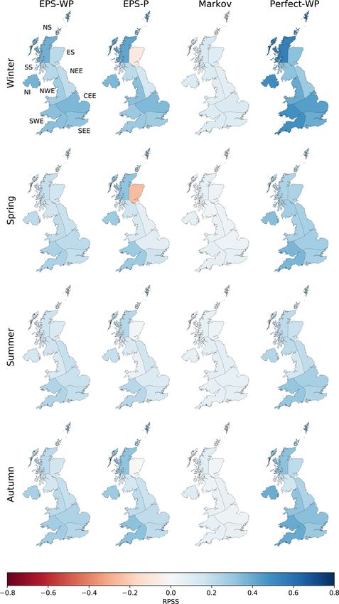
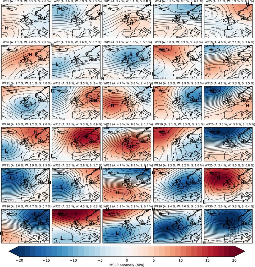
108                                   D. Richardson et al.: Improving sub-seasonal forecast skill of meteorological drought

   Weather pattern (WP; also called weather types, circula-         to this study, Lavaysse et al. (2018) predicted monthly me-
tion patterns and circulation types) classifications are a candi-   teorological drought in Europe using a WP-based method.
date for such an application. A WP classification consists of       They aggregated ECMWF-EPS daily reforecasts of WPs to
a number of individual WPs, which are typically defined by          predict monthly frequency anomalies of each WP. For each
an atmospheric variable and represent the broad-scale atmo-         1◦ grid cell, the predictor was chosen to be the WP that
spheric circulation over a given domain (Huth et al., 2008).        corresponded to the maximum absolute temporal correlation
They can be used to make general predictions of local-scale         between the monthly WP frequency-of-occurrence anomaly
variables such as wind speed, temperature and precipitation         and the monthly standardised precipitation index (SPI; Mc-
and are a tool for reducing atmospheric variability to a few        Kee et al., 1993). Using this relationship, the model predicted
discrete states. WP classifications have mainly been studied        drought in a grid cell when 40 % of the ECMWF-EPS ensem-
in the context of extreme hydro-meteorological events (Hay          ble members forecast an SPI value below −1. Compared to
et al., 1991; Wilby, 1998; Bárdossy and Filiz, 2005; Richard-       direct ECMWF-EPS drought forecasts, the WP-based model
son et al., 2018, 2019a) and as a tool for analysing historical     was more skilful in north-eastern Europe during winter but
and future changes in atmospheric circulation patterns (Hay         less skilful for central and eastern Europe during spring and
et al., 1992; Wilby, 1994; Brigode et al., 2018). See Huth et       summer. Over the UK, the WP model appeared to be superior
al. (2008) for a comprehensive review of WP classifications.        for north-western regions in winter but inferior in summer,
   Until recently, the capability of dynamical models to pre-       although scores for the latter were of low magnitude.
dict WP occurrences had been little researched. Ferranti               The aforementioned studies have all considered
et al. (2015) evaluated the forecast skill of the medium-           daily WPs. An example of WPs defined on the sea-
range European Centre for Medium-Range Weather Fore-                sonal timescale was presented by Baker et al. (2018). The
casts ensemble prediction system (ECMWF-EPS; Buizza                 authors analysed reforecasts of UK regional winter precip-
et al., 2007; Vitart et al., 2008) using WPs. They objec-           itation between the winters of 1992–1993 and 2011–2012
tively defined four WPs according to daily 500 hPa geopoten-        using GloSea5, which has little raw skill in forecasting this
tial heights over the North Atlantic–European sector. Model         variable (MacLachlan et al., 2015). GloSea5 has, however,
forecasts of this variable for October through April be-            been shown to skilfully forecast the winter NAO (Scaife et
tween 2007 and 2012 were then assigned to the closest               al., 2014). Baker et al. (2018) exploited this by constructing
matching WP using the root-mean-square difference. Ver-             two winter MSLP indices over Europe and the North
ification scores indicated that there was superior skill for        Atlantic, and reforecasts of these indices were derived from
predictions initialised during negative phases of the North         the raw MSLP fields. A simple regression model then related
Atlantic Oscillation (NAO; Walker and Bliss, 1932). Simi-           these indices to regional precipitation and produced more
larly, WPs were used to evaluate the skill of the Antarctic         skilful forecasts than the raw model output.
Mesoscale Prediction System by Nigro et al. (2011).                    In this study, we explore the potential for utilising a
   To support weather forecasting in the UK in the medium           WP classification (specifically MO30) in UK meteorological
to long range, the Met Office uses a WP classification,             drought prediction. We predict WPs using two models, the
MO30, in a post-processing system named “Decider” (Neal             ECMWF-EPS and a Markov chain, from which precipita-
et al., 2016). Using a range of ensemble prediction systems,        tion and drought forecasts are derived. These models will be
forecast mean sea-level pressure (MSLP) fields over Eu-             compared to direct precipitation and drought forecasts from
rope and the North Atlantic Ocean are assigned to the best-         ECMWF-EPS. We also run an idealised, perfect-prognosis
matching WP according to the sum of squared differences be-         model that uses WP observations rather than forecasts as an
tween the forecast MSLP anomaly and WP MSLP anomaly                 “upper benchmark” to assess the upper limit of the usefulness
fields. Decider therefore produces a probabilistic prediction       of the WP classification. Section 2 contains details of the data
of WP occurrences for each day in the forecast lead time.           sets used, including describing the creation of a WP refore-
Decider has various operational applications: predicting the        cast data set. Section 3 describes the models in detail and the
possibility of flow transporting volcanic ash originating in        forecast verification procedure. In Sect. 4, we present the re-
Iceland into UK airspace, highlighting potential periods of         sults, and in Sect. 5, we draw some conclusions and make
coastal flood risk around the British Isles (Neal et al., 2018),    recommendations for future work.
and acting as an early-forecast system for fluvial flooding
(Richardson et al., 2019b).
   For Japan, Vuillaume and Herath (2017) defined a set             2   Data
of WPs according to MSLP. These WPs were used to refine
bias-correction procedures, via regression modelling, of pre-       We use a Met Office WP classification called MO30 (Neal
cipitation from two global ensemble forecast systems. The           et al., 2016). WPs in MO30 were defined by using simulated
authors found that improvements from the bias-correction            annealing to cluster 154 years (1850–2003) of daily MSLP
method using WPs were strongly dependent on the WP but              anomaly fields into 30 distinct states. The data were extracted
overall superior to the global (non-WP) method. Relevant            from the European and North Atlantic daily to multidecadal

Nat. Hazards Earth Syst. Sci., 20, 107–124, 2020                             www.nat-hazards-earth-syst-sci.net/20/107/2020/
D. Richardson et al.: Improving sub-seasonal forecast skill of meteorological drought                                                   109

climate variability (EMULATE) data set (Ansell et al., 2006)       Table 1. Range of daily precipitation, x, for each bin pb and of 16,
in the domain 35–70◦ N, 30◦ W–20◦ E, with a spatial resolu-        31 and 46 d total precipitation, y, for each bin sc .
tion of 5◦ latitude and longitude. These 30 WPs are there-
fore representative of the 30 most common patterns of daily                  Daily precipitation        Total 16, 31 and 46 d precipitation
atmospheric circulation over Europe and the North Atlantic             pb     Range of precipitation,   sc    Range of summed
(Fig. 1), and they were ordered such that WP1 is the most                     x (mm)                          precipitation, y (mm)
frequently occurring WP annually, while WP30 is the least              p1     0                         s1    0 < y ≤ 10
frequent. A consequence of the clustering process and order-           p2     0
110                                   D. Richardson et al.: Improving sub-seasonal forecast skill of meteorological drought

Figure 1. Weather pattern (WP) definitions according to mean sea-level pressure (MSLP) anomalies (hPa). The black contours are isobars
showing the absolute MSLP values associated with each weather pattern, with the centres of high and low pressure also indicated. Next to
the WP labels are the annual (A), winter (W; DJF) and summer (S; JJA) relative frequencies of occurrences of each WP (%). The frequency-
of-occurrence data are associated with the WPs based on ERA-Interim between 1979 and 2017, while the WP definitions were generated
from a clustering process applied to EMULATE MSLP reanalysis data between 1850 and 2003. See the text for details.

Nat. Hazards Earth Syst. Sci., 20, 107–124, 2020                                www.nat-hazards-earth-syst-sci.net/20/107/2020/
D. Richardson et al.: Improving sub-seasonal forecast skill of meteorological drought                                                         111

not widespread, although there is some published research                    Precipitation is estimated from the WP predictions (or
on the topic (Leung and North, 1990; Kleeman, 2002; Roul-                 observations in the case of Perfect-WP) by sampling from
ston and Smith, 2002; Ahrens and Walser, 2008; Weijs et                   the conditional distributions of precipitation given each Era-
al., 2010; Weijs and v. d. Giesen, 2011). The JSD will be                 Interim WP between 1979 and 2017. We process the daily
used to measure the forecast performance by quantifying the               HadUKP precipitation data by discretising into v bins with
distance between distributions of the observed and forecast               historical probabilities pb for b = 1, . . . , v. Dry days form
WP frequencies. The JSD is based on the Kullback–Leibler                  one bin, and bin intervals increase for higher precipitation
divergence (KLD; Kullback and Leibler, 1951). Let P and                   values (Table 1). This gives a discrete distribution of pre-
Q be two discrete probability distributions. The KLD from Q               cipitation interval relative frequencies, D(z), with condi-
to P is given by                                                          tional distributions for each WP given by D(z|W = i), for
                                                                          i = 1, . . . , 30. We also define w summed precipitation in-
                    I
                    X               Qi                                    tervals sc for c = 1, . . . , w. Forecast probabilities of these
DKL (P ||Q) = −           Pi log2      ,                           (1)
                                    Pi                                    summed intervals are derived from the WP forecast models
                    i=1
                                                                          as follows.
measured in bits (i.e. a binary unit of information). In
                                                                           1. Set the ensemble member e ∈ (e1 , . . . , eNe ), where Ne is
our application I = 30, the number of WPs and P =
                                                                              the number of ensemble members, and time to t = 0,
(pf,1 , . . . , pf,30 ) and Q = (qf,1 , . . . , qf,30 ) are the vectors
                                                                              the first day of the forecast. Then the predicted WP
of observed and forecast WP relative frequencies,         P respec-           by ensemble member e at time t is We (t) = i for i =
tively.  (Because      these are relative frequencies,       P = 1 and
P                                                                             1, . . . , 30.
   Q = 1.) As there would inevitably be some cases where
the model predicts no occurrences of some WPs (i.e. when                   2. Set p0 = 0 and calculate the probabilities p1 , . . . pm of
Q contains zeros), DKL (P ||Q) will be undefined at times.                    each of the m daily precipitation bins from the discrete
Using the JSD avoids this problem; it is defined as                           precipitation distribution that is conditional on We (t)
                                                                              and on the 91 d windows centred on t (i.e. t −45, . . . , t +
              1             1
DJSD (P ||Q) = DKL (P ||M) + DKL (Q||M),                           (2)        45) from every year except the current year. This last
              2             2                                                 condition is equivalent to a leave-one-year-out cross-
where M = (P + Q)/2. Unlike the KLD, the JSD is                               validation procedure.
symmetric, i.e. DJSD (P ||Q) ≡ DJSD (Q||P ). Also, 0 ≤
                                                                           3. Define the maximum value of each bin as lpb , b =
DJSD (P ||Q) ≤ 1, with a score of zero indicating that P and
                                                                              1, . . . , v, with lp0 = 0. Note that lp0 = lp1 = 0, ensuring
Q are the same (a perfect forecast). Equation (2) gives the
                                                                              that zero precipitation days can be simulated.
JSD for a single forecast–event pair; to obtain the average
JSD for all forecasts, we take the mean of all forecast–event              4. Generate u random variables pk∗ ∼ U (0, 1) for k =
pairs. Skill is evaluated separately for each month, with the                 1, . . . , u.
middle date of each forecast period used to assign the month.
                                                                                                                                    q
We calculate forecast skill for lead times of 16, 31 and 46 d.             5. For each pk∗ , find the index q such that
                                                                                                                                    P
                                                                                                                                        pj < pk∗ <
We use the JSD to compare WP forecast skill of EPS-WP and                                                                        j =0
the Markov model, considering each lead time separately.                       q+1
                                                                               P                      q−1
                                                                                                      P                      q
                                                                                                                             P
                                                                                      pj . Set Pq =          pj and Pq+1 =          pj , the cumu-
3.2   Precipitation and drought forecast models                                j =0                   j =0                   j =0
                                                                               lative probabilities of the bins adjacent to pk∗ .
We compare four models, three of which are forecast mod-
                                                                           6. Define the difference between the adjacent bins as α =
els while one model is a perfect-prognosis model. Figure 2
                                                                              Pq+1 − Pq and the difference between the random num-
shows a schematic of the procedure involved in generating
                                                                              ber and the lower cumulative probability as β = pk∗ −
forecasts from each model. All models are considered at the
                                                                              Pq .
same lead times to be the WP predictions. Two of the forecast
models are driven first by a WP component: EPS-WP and                      7. Estimate the precipitation value for each pk∗ as rk (t) =
the Markov model described above. The perfect-prognosis                       lpq + βα (lpq+1 −lpq ). We now have u predicted daily pre-
model, Perfect-WP, is used as an “upper benchmark” with                       cipitation values at time t, r(t) = (r1 (t), . . . , rn (t)).
(future) observed WPs as input rather than forecast WPs.
It is an idealised model that cannot be used operationally,                8. Set t = t + 1 and repeat steps 3 to 6 until the final day
but it allows us to assess the potential usefulness of WPs in                 of the forecast, tmax , is processed.
precipitation and drought forecasting. Note that from here,
any reference to drought refers specifically to meteorological             9. Sum the daily precipitation
                                                                                                  P       vectors and divide by the
drought.                                                                      random sample size ( r(t))/u for τ = 0, . . . , tmax .
                                                                                                             τ

www.nat-hazards-earth-syst-sci.net/20/107/2020/                                       Nat. Hazards Earth Syst. Sci., 20, 107–124, 2020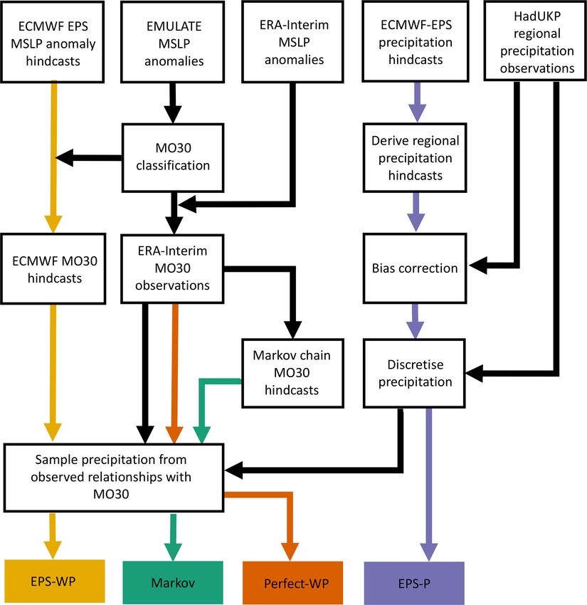
112 D. Richardson et al.: Improving sub-seasonal forecast skill of meteorological drought
Figure 2. Schematic showing the procedure for the four precipitation forecast models. The top row shows the base data sets used, and the
bottom row shows the four models. Coloured arrows begin at the first stage for which forecasts are issued: EPS-WP forecasts begin with the
ECMWF prediction system MSLP forecasts, Markov forecasts are produced once the ERA-Interim MO30 time series has been derived, and
Perfect-WP “forecasts” are observations from the same time series, while EPS-P forecasts are the post-processed data from the ECMWF
forecast system.
10. Discretise according to the w summed precipita- 10 000. The fourth model (the third forecast model) is the
tion bins s1 , . . . , sw to obtain a distribution of rel- direct ECMWF-EPS precipitation forecasts (EPS-P), pro-
ative frequencies for this ensemble member f e,c = cessed to provide probabilistic predictions of regional pre-
(fe,1 , . . . , fe,w ). cipitation intervals as described earlier.
11. Set a new ensemble member e∗ ∈ (e1 , . . . , eNe ), with 3.3 Precipitation forecast verification
e∗ 6 = e and repeat steps 2 to 10 until every ensemble
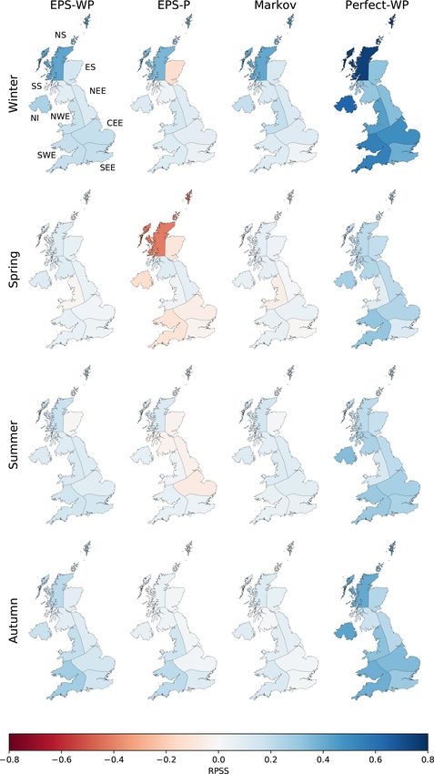
member has been processed. To evaluate precipitation forecast performance, we use the
ranked probability score (RPS; Epstein, 1969; Murphy,
12. Sum each ensemble member’s distribution of summed
1971). We express the RPS as the ranked probability skill
precipitation relative frequencies (element-wise) and di-
score (RPSS) using
vide by the number of ensemble members P to obtain a fi-
nal forecast probability distribution: F = ( f e,c )/Ne . RPS
e RPSS = 1 − , (3)
RPSref
The number of ensemble members depends on the model.
For EPS-WP, Ne = 11, i.e. the number of ensemble mem- where RPSref is the score of a climatological forecast, which
bers of the ECMWF dynamical model. For the Markov in our case is the climatological event category (i.e. precip-
model Ne = 1000. We set the number of samples drawn itation interval) relative frequencies (PC). A perfect score is
from each WP-precipitation conditional distribution as u = achieved when RPSS = 1, which is also the upper limit. Neg-
Nat. Hazards Earth Syst. Sci., 20, 107–124, 2020 www.nat-hazards-earth-syst-sci.net/20/107/2020/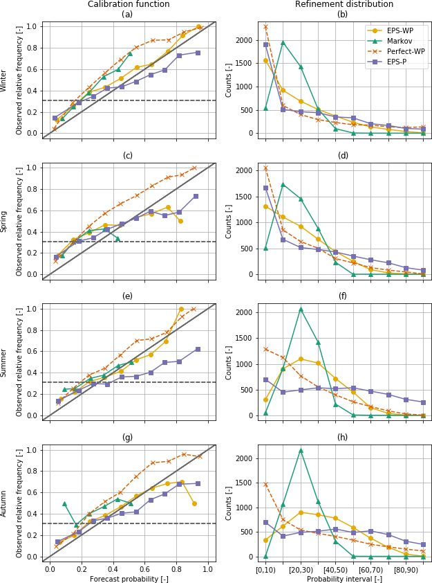
D. Richardson et al.: Improving sub-seasonal forecast skill of meteorological drought 113
ative (positive) values indicate that the forecast is performing mean of all forecast probabilities in each bin is the value plot-
worse (better) than RPSref . ted on the diagrams (Bröcker and Smith, 2007). Points along
the 1 : 1 line represent a well-calibrated, reliable, forecast, as
3.4 Drought forecast verification event probabilities are equal to the forecast probabilities and
suggest that we can interpret our forecasts at “face value”. If
We evaluate model performance in predicting dichotomous the points are to the right (left) of the diagonal, the model is
drought or non-drought events. We define two classes of over-forecasting (under-forecasting) the number of drought
drought severity. The first class, mild drought, is when pre- events.
cipitation sums (over the length of the considered lead time: The forecast resolution can also be deduced from the cal-
either 16, 31 or 46 d) are below the 30.9th percentile of the ibration function. For a forecast with poor resolution, the
summed precipitation distribution. The second class is mod- event relative frequencies g(o1 |pi ) only weakly depend on
erate drought, with such sums being below the 15.9th per- the forecast probabilities. This is reflected by a smaller dif-
centile. These percentiles are calculated for each region and ference between the calibration function and the horizontal
month using the whole data set from 1979 to 2017 and are line of the climatological event frequencies and suggests that
chosen as they correspond to SPI values of −0.5 and −1, the forecast is unable to resolve when a drought is more or
respectively. less likely to occur than the climatological probability. Good
resolution, on the other hand, means that the forecasts are
3.4.1 The Brier skill score
able to distinguish different subsets of forecast occasions for
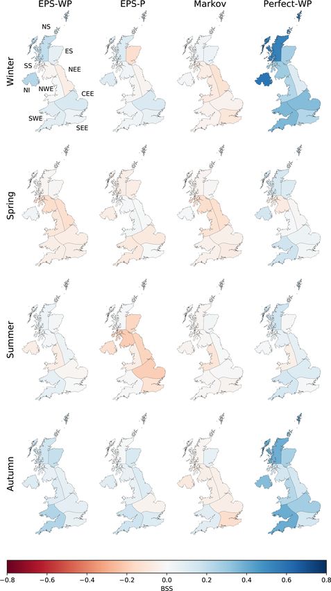
We use three verification techniques to assess skill in predict- which the subsequent event outcomes are different to each
ing droughts. The first is the Brier skill score (BSS). The BSS other.
is based on the Brier score (BS; Brier, 1950), which measures The second element of reliability diagrams is the refine-
the mean-square error of probability forecasts for a dichoto- ment distribution, g(pi ). This expresses how confident the
mous event, in this case the occurrence or non-occurrence of forecast models are by counting the number of times a fore-
drought. The BS is converted to a relative measure, or skill cast is issued in each probability bin. This feature is also
score, by setting called sharpness. A low-sharpness model would overwhelm-
ingly predict drought at the climatological frequency, while
BS a high-sharpness model would forecast drought at extreme
BSS = 1 − , (4)
BSref high and low probabilities, reflecting its level of certainty
with which a drought will or will not occur, independent of
where BSref is the score of a reference forecast given by the whether a drought actually does subsequently occur or not.
quantiles associated with each drought threshold, 0.309 for
mild drought and 0.159 for moderate drought. As with the 3.4.3 Relative operating characteristics
RPSS, a perfect score is achieved when BSS = 1 and nega-
tive (positive) values indicate that the forecast is performing As a final diagnostic, we use the relative operating char-
worse (better) than BSref . acteristic (ROC) curve (Mason, 1982; Wilks, 2011), which
visualises a model’s ability to discriminate between events
3.4.2 Reliability diagrams – forecast reliability, and non-events. Conditioned on the observations, the ROC
resolution and sharpness curve may be considered a measure of potential usefulness
– it essentially asks what the forecast is given that a drought
The BS can be decomposed into reliability, resolution and has occurred. The ROC curve plots the hit rate (when the
uncertainty terms (Murphy, 1973): model forecasts a drought and a drought subsequently oc-
curs) against the false alarm rate (when the model forecasts
BS = reliability − resolution + uncertainty, (5)
a drought but a drought does not then occur). We compute
enabling a more in-depth assessment of forecast model per- the hit rate and false alarm rate for cumulative probabilities
formance. Reliability diagrams offer a convenient way of vi- between 0 % and 100 % at intervals of 10 %. A skilful fore-
sualising the first two of these terms (Wilks, 2011). These cast model will have a hit rate greater than a false alarm rate,
diagrams consist of two parts, which together show the full and the ROC curve would therefore bow towards the top-
joint distribution of forecasts and observations. The first el- left corner of the plot. The ROC curve of a forecast system
ement is the calibration function, g(o1 |pi ) for i = 1, . . . , n, with no skill would lie along the diagonal, as the hit rate and
where o1 indicates the event (here, a drought) occurring, and false alarm rate would be equal, meaning that the forecast
the pi values are the forecast probabilities. The calibration is no better than a random guess. The area under the ROC
function is visualised by plotting the event relative frequen- curve (AUC) is a useful scalar summary. The AUC ranges be-
cies against the forecast probabilities and indicates how well tween zero and 1, with higher scores indicating greater skill.
calibrated the forecasts are. We split the forecast probabili-
ties into 10 bins (subsamples) of 10 % probability, and the
www.nat-hazards-earth-syst-sci.net/20/107/2020/ Nat. Hazards Earth Syst. Sci., 20, 107–124, 2020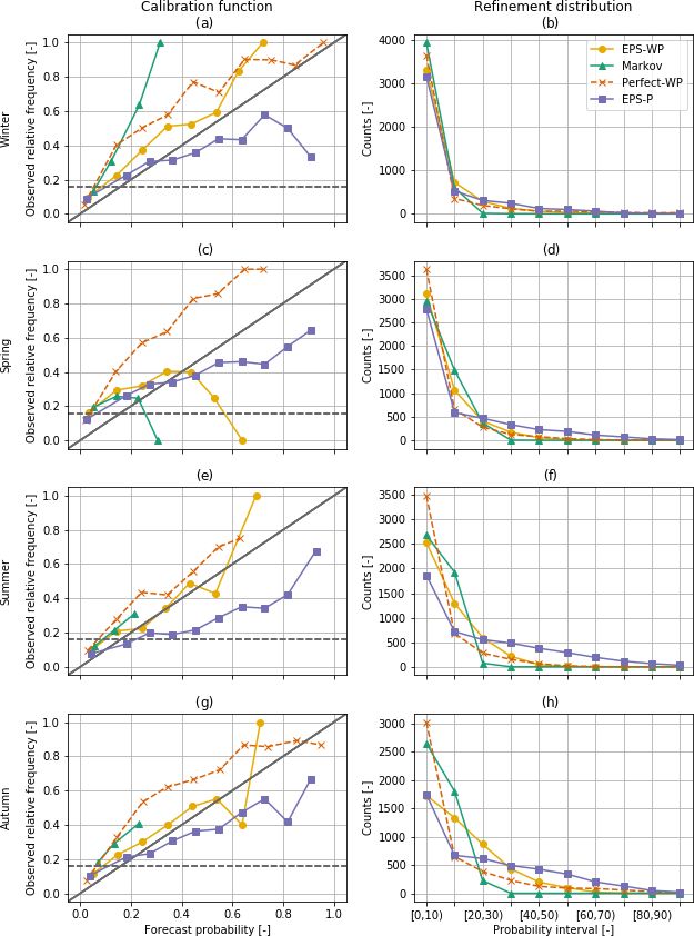
114                                   D. Richardson et al.: Improving sub-seasonal forecast skill of meteorological drought

Figure 3. Jensen–Shannon divergence scores for EPS-WP and Markov models for three lead times.

4     Results                                                        is noteworthy for highlighting the behaviour of the Markov
                                                                     model.
To reduce information overload, we do not show results for              We could have assessed model skill in predicting the WPs
every combination of region, lead time and drought class.            using more common metrics such as the BS, which could
Key results not shown will be conveyed via the text. We ag-          measure the hit / miss ratio for each WP at each lead time.
gregate the precipitation results from monthly to 3-month            However, the focus of this paper is on multi-week precipi-
seasons for visual clarity and combine regional results for          tation (and drought) totals, so we are not particularly inter-
the ROC and reliability diagrams for the same reason.                ested in the models’ ability to predict the timing of a WP,
                                                                     only whether they are able to capture the distribution of the
4.1    WP forecasts                                                  WP frequencies of occurrence. It is likely that using the
                                                                     BS would show that EPS-WP and Markov skill decreases
We find that EPS-WP is more skilful at predicting the WPs
                                                                     with lead time, as was the case for a WP classification de-
than the Markov model for every month and every lead time,
                                                                     rived from MO30 by Neal et al. (2016).
although the difference in skill between the two models de-
creases as the lead time increases. The skill difference be-         4.2   Precipitation forecasts
tween models is much larger for a lead time of 16 d com-
pared to a lead time of 46 d (Fig. 3). For a 46 d lead time, the     We first discuss the skill of the three true forecast models,
difference in skill is negligible for May through October; in        EPS-WP, EPS-P and Markov. For the most part, all three
fact, these months have the smallest differences in JSD for all      models are more skilful than climatology independent of sea-
lead times. This is presumably because the summer months             son and lead time, with greater skill in autumn and winter
are associated with fewer WPs compared to winter (Richard-           compared to spring and summer (Figs. 4 and 5). For a 16 d
son et al., 2018), resulting in a more skilful Markov model          lead time, there is little to choose between EPS-WP and EPS-
due to higher transition probabilities.                              P, except in ES, for which the latter model is less skilful than
   An interesting result is how JSD scores for Markov de-            climatology in winter and spring (Fig. 4). Markov is the least
crease as the lead time increases (Fig. 3), suggesting an im-        skilful model at this lead, offering only a marginal improve-
provement in skill with lead time. This is the opposite of the       ment on climatology (Fig. 4). The skill of EPS-WP and EPS-
expected (and usual) effect. The Markov model predicts WPs           P reduces when a 31 d lead is considered, bringing their skill
using the 1 d transition probabilities, and its ensemble mem-        more into line with Markov (Fig. S2). At a 46 d lead the dif-
bers therefore diverge very quickly, resulting in a distribu-        ferences are starker, with EPS-P being notably less skilful
tion of predicted WPs that looks similar to the climatologi-         than EPS-WP, Markov and climatology for many regions in
cal WP distribution for all lead times. For a 16 d forecast, the     summer and, especially, spring (Fig. 5). These results are,
observed WP distribution of the corresponding 16 d will gen-         however, still only marginally superior to climatology. EPS-
erally be less similar to the climatological WP distribution         WP has greater skill than EPS-P at this lead time in winter
than for 31 d forecasts and less similar still than for 46 d fore-   and autumn for NS, NI, CEE and SWE, although the magni-
casts. For instance, at a 16 d lead, only 16 unique WPs could        tudes of these differences are small (Fig. 5). There is little ev-
form the observed distribution, whereas Markov is capable of         idence of coherent regional variability in model skill, except
predicting all possible WPs across its 1000 members at this          perhaps a tendency for EPS-P to score more highly for west-
lead. As the JSD measures the distance between these prob-           ern regions in spring and summer at a 16 d lead time (Fig. 4).
ability distributions, it tends to score the differences between     Despite low skill relative to climatology at longer lead times,
these distributions as more similar (a smaller divergence) for       there is clearly some benefit to using the WP-based models
longer lead times. This means that the JSD is perhaps not ap-        (particularly EPS-WP) for certain regions and seasons.
propriate as a verification metric in an operational sense but

Nat. Hazards Earth Syst. Sci., 20, 107–124, 2020                              www.nat-hazards-earth-syst-sci.net/20/107/2020/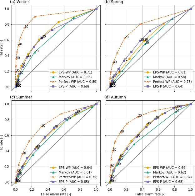
D. Richardson et al.: Improving sub-seasonal forecast skill of meteorological drought                                           115

Figure 4. The ranked probability skill score (RPSS) for precipita-   Figure 5. As Fig. 4 but for a 46 d lead.
tion forecasts at a 16 d lead for each model and season.

                                                                     4.3     Meteorological drought forecasts
   The potential usefulness of such approaches is high-
lighted by the performance of Perfect-WP. Unsurprisingly,            4.3.1    Forecast accuracy
this model is almost uniformly the most skilful model for
all regions, seasons and lead times (Figs. 4, 5 and S2). The         Forecast accuracy is typically lower for mild drought (total
gains in skill for this model over the other three models are        precipitation over 16, 31, or 46 d below the 30.9th percentile)
most pronounced during winter and autumn and especially              than for precipitation and lower still for moderate drought
for longer lead times. Skill is greatest for most western re-        (total precipitation below the 15.9th percentile). The regional
gions (NS, NI, NWE and SWE) and lowest for eastern re-               and lead-time differences in precipitation skill are also evi-
gions ES, NEE and SEE, together with SS (Fig. 5). Perfect-           dent for drought, with higher skill at shorter leads and dur-
WP is obviously not practical, but the results serve to show         ing winter and autumn (Figs. 6, 7 and S3). Results for mild
that WPs are a potentially useful tool in medium-range pre-          drought are not shown, as they generally lie in between those
cipitation forecasting.                                              for precipitation (Figs. 4, 5 and S2) and moderate drought
                                                                     (Figs. 6, 7 and S3). Markov again has the poorest skill, with
                                                                     a climatology forecast preferable for many combinations of
                                                                     region and lead time. EPS-P is either equal to or more skil-

www.nat-hazards-earth-syst-sci.net/20/107/2020/                                 Nat. Hazards Earth Syst. Sci., 20, 107–124, 2020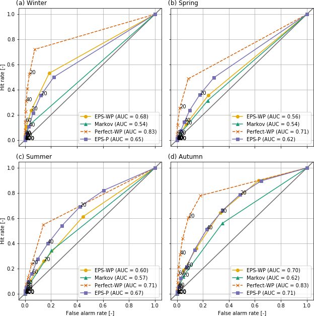
116 D. Richardson et al.: Improving sub-seasonal forecast skill of meteorological drought
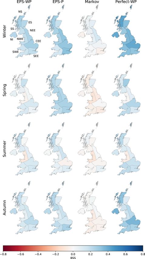
Figure 6. The Brier skill score (BSS) for mild drought (total pre- Figure 7. As Fig. 6 but for a 46 d lead.
cipitation below the 30.9th percentile) for a 16 d lead time for each
model and season.
46 d lead time (Fig. 7). For winter and autumn, however, the
skill is reasonable UK-wide and particularly high during win-
ful than EPS-WP at a 16 d lead (Fig. 6) and during spring ter in NS and NI (Fig. 7). The same east–west skill split is
for longer leads (Figs. 7 and S3). Conversely, EPS-WP out- present for moderate drought as it was for precipitation, with
performs EPS-P during summer at the longer two lead times, some western regions benefitting from higher skill than east-
although a climatology forecast would be just as, if not more, ern regions (Fig. 7).
skilful. As with precipitation forecasts, any gain in skill using
EPS-WP over EPS-P in winter and autumn at longer leads is 4.3.2 Relative operating characteristics
marginal, with both models showing more skill than clima-
tology (Figs. 7 and S3). All models are better able to discriminate between drought
Skill, where present, is undeniably modest, but the rel- and non-drought events than random chance, with Perfect-
atively high skill of Perfect-WP in some regions and sea- WP being the most able and Markov the least able, subject to
sons again shows the potential predictability of drought us- similar caveats regarding lead time and season as for the BSS
ing WP methods. Compared to precipitation forecasts, skill and RPSS results. During summer and spring, EPS-P has the
for Perfect-WP is notably lower for spring and summer, with highest AUC of any of the three forecast models (Figs. 8
climatology often being a competitive forecast method at a and 9) and for a 16 d lead-time scores similarly to Perfect-WP
Nat. Hazards Earth Syst. Sci., 20, 107–124, 2020 www.nat-hazards-earth-syst-sci.net/20/107/2020/D. Richardson et al.: Improving sub-seasonal forecast skill of meteorological drought 117
Figure 8. Relative operating characteristic (ROC) curves and area under ROC curve (AUC) for mild drought with a 46 d lead time. Annotated
values indicate drought forecast probability thresholds.
(not shown). On the other hand, EPS-WP is the best discrim- rate. For mild drought, a 20 % probability threshold for EPS-
inator during winter and autumn at a 46 d lead time, although WP and EPS-P achieves at least 60 % hit rates at all lead
the magnitude of the differences is small (Figs. 8 and 9). times, whereas for moderate drought, this threshold will only
Markov is consistently the least suitable model for predicting achieve such hit rates at a 16 d lead time during winter and
drought according to the ROC curve, although it still repre- autumn (EPS-P also achieves this rate for spring and sum-
sents a better method of doing so than random chance. mer; not shown) and during autumn for all lead times. In gen-
A use of the ROC curve is to provide end users with in- eral, it appears that these low probability thresholds yield the
formation on how to apply the considered forecast models. best compromise between hits and false alarms, although in
As the plotted points on each curve indicate the hit rate practice, the costs (e.g. financial) associated with false alarms
and false alarm rate associated with predicting droughts at and missed events will determine how responders use these
each probability interval, they can be used to make an in- probabilities.
formed decision in selecting a probability threshold for is-
suing a drought forecast. For example, should a forecaster 4.3.3 Forecast reliability, resolution and sharpness
choose to issue a moderate drought warning in winter at a
10 % probability level and 46 d lead time (Fig. 9), then they EPS-WP is the most reliable forecast model (i.e. excluding
would expect EPS-WP to achieve a hit rate over double that Perfect-WP), and while all three WP-driven forecast mod-
of the false alarm rate (∼ 55 % and ∼ 20 %, respectively). els tend to under-forecast droughts, EPS-P only does so for
EPS-P, meanwhile, shows a slightly lower hit rate and similar lower probability thresholds, with the higher thresholds re-
false alarm rate (∼ 50 % and ∼ 20 %). The idealised bench- sulting in this model over-forecasting. This is particularly
mark model (Perfect-WP) achieves an outstanding score – an true for shorter lead times and during winter, although it
over 70 % hit rate compared to a less than 10 % false alarm is still clear for 31 d lead times in some seasons (Figs. 10
and 11). Sometimes EPS-WP follows the same pattern as
www.nat-hazards-earth-syst-sci.net/20/107/2020/ Nat. Hazards Earth Syst. Sci., 20, 107–124, 2020118 D. Richardson et al.: Improving sub-seasonal forecast skill of meteorological drought Figure 9. As Fig. 8 but for moderate drought. EPS-P and over-forecasts drought occurrence for higher pre- drought (Fig. 10) and 60 % for moderate drought (except in dicted probabilities (e.g. Figs. 10c, e and g and 11c). How- spring; Fig. 11), despite having lower accuracy (e.g. Fig. 6). ever, the total number of forecasts issued in these inter- As a more skilful BSS is composed of smaller reliability vals is generally smaller than for EPS-P, as the refinement and larger resolution terms (Kharin and Zwiers, 2003), it fol- distributions show most clearly for mild drought (Fig. 10). lows that the resolution of Perfect-WP is sufficiently large to This means that the corresponding points of the calibration overcome the larger reliability term compared to EPS-WP function are less reliable for EPS-WP (and Markov) due to and yield an overall more accurate forecast model. How- smaller sample sizes (Bröcker and Smith, 2007). In fact, all ever, for drought forecasts issued with higher probabilities, three WP-based models have occasions when there are no EPS-WP is the less reliable model, under- or over-forecasting issued forecasts with certain probabilities. These are high drought (depending on the season) more than Perfect-WP. probabilities for Perfect-WP and EPS-WP (Fig. 11c and e) These under- or over-forecasting biases must be taken into but can be as low as between 30 % and 40 % for Markov account by an operational forecaster using these models. (Fig. 11e and g). As such, although EPS-WP appears to be A key difference apparent from the calibration function the most reliable model from looking only at the calibra- relates to the ability of the models to identify subsets of fore- tion function, there is less certainty of this fact for moderate cast situations where the subsequent event relative frequen- drought and for higher forecast probabilities. This erratic be- cies are different, i.e. the forecast resolution. A fairly consis- haviour of the conditional event relative frequencies is most tent feature across all lead times and drought classes is the obvious in Fig. 11c and is explained by the very low sample poorer resolution of EPS-P, particularly obvious in summer sizes of forecasts issued with anything but a small probability (Figs. 10e and 11e), with the conditional event relative fre- (Fig. 11e; Wilks, 1995). An interesting result is that forecasts quencies quite clearly closer to the climatological average from EPS-WP are more reliable than from Perfect-WP when compared to the other models. This should be considered the predicted drought probabilities are below 80 % for mild in conjunction with the sharpness of the forecast, which is Nat. Hazards Earth Syst. Sci., 20, 107–124, 2020 www.nat-hazards-earth-syst-sci.net/20/107/2020/
D. Richardson et al.: Improving sub-seasonal forecast skill of meteorological drought                                                         119

Figure 10. Calibration functions (first column) and refinement distributions (second column) for mild drought with a 31 d lead time. For the
calibration function diagrams, the solid diagonal line indicates perfect reliability and the dashed horizontal line is the event relative frequency
for mild drought (0.309).

relatively high for this model as shown by the numbers of                   whelmingly predicting droughts at the climatological fre-
issued extreme probabilities, particularly those in the upper               quency (second column of Figs. 10 and 11). This means that
tail (Figs. 10f and 11f). This combination of poor resolution               the Markov model is not a useful operational tool in these sit-
and high sharpness indicates “overconfidence” (Wilks, 2011)                 uations, as similar forecasts could be obtained simply by us-
– on the occasions that EPS-P issues a forecast indicating the              ing the climatological drought frequency. The refinement dis-
likelihood of a drought is very high, the actual likelihood of a            tributions for EPS-WP show that for mild drought in winter
drought subsequently occurring is lower. To compensate for                  and spring and for moderate drought in all seasons, the model
this overconfidence, a user would adjust the probabilities to               predicts droughts with low probabilities the majority of the
be less extreme to make the forecasts more reliable.                        time (Figs. 10b and d and 11b, d, f and h). For mild drought
   We can compare these refinement distributions to those                   in summer and autumn, however, this model mostly issues
of the Markov model, which exhibits low sharpness, over-                    forecasts close to the climatological frequency, although not

www.nat-hazards-earth-syst-sci.net/20/107/2020/                                        Nat. Hazards Earth Syst. Sci., 20, 107–124, 2020
120                                    D. Richardson et al.: Improving sub-seasonal forecast skill of meteorological drought

Figure 11. As Fig. 10 but for moderate drought (event relative frequency of 0.159).

nearly as regularly as the Markov model (Fig. 10f and h). As            WP predictions, we derived precipitation and meteorological
with adjusting for bias, a forecaster can use model resolution          drought forecasts and compared them to direct precipitation
and sharpness when assessing drought forecast probabilities             and drought predictions from the dynamical system (EPS-
output by a model.                                                      P). We compared two levels of drought: mild drought, when
                                                                        the total precipitation over the lead time (16, 31 or 46 d)
                                                                        was below the 30.9th percentile climatology, and moderate
5   Discussion and conclusions                                          drought, when the total precipitation over the lead time was
                                                                        below the 15.9th percentile. Overall, forecast models were
We have compared the performance of a dynamical forecast                found to be more skilful during winter and autumn, partic-
system (EPS-WP) and a first-order Markov model in pre-                  ularly for longer lead times. The Markov model tended to
dicting WP occurrences over a range of lead times, showing              be the least skilful, especially when predicting drought. Dif-
that the dynamical model is always more skilful, although               ferences in skill between EPS-P and EPS-WP were typically
the difference in skill reduces with lead time. From these

Nat. Hazards Earth Syst. Sci., 20, 107–124, 2020                                  www.nat-hazards-earth-syst-sci.net/20/107/2020/
D. Richardson et al.: Improving sub-seasonal forecast skill of meteorological drought 121
small, with RPSS, BSS and ROC results not highlighting a cipitation are well represented in these seasons. The lesser
clear winner. However, we demonstrated the potential in im- skill of EPS-WP and Markov, then, is a result of poor pre-
proving WP forecasts further by showing that an idealised, diction of the WPs. A focus on improving the skill of the
perfect-prognosis model (Perfect-WP) would provide much WP forecasts could be the most useful route to improving
more skilful precipitation and drought forecasts, with high precipitation and drought predicting skill. Currently, dynam-
hit rates and low false alarm rates. ical models such as the ECMWF system used here represent
From assessing reliability diagrams, we found that WP- the best method of predicting WPs. Moreover, the ECMWF
based models only issue binary drought forecasts with ei- reforecast data used here had 11 ensemble members, whereas
ther very low probabilities or probabilities close to the cli- the operational forecasts are run with 51 members. There-
matological average. In particular, there is little to gain in fore, an operationalised version of the models might improve
using the Markov model in mild drought prediction over the forecast skill or better represent uncertainty, although this is
climatological frequency, as it tends to issue drought fore- also true for precipitation forecasts direct from the model. A
casts with this probability anyway. EPS-P has the highest useful piece of further research would be to assess the fore-
sharpness, predicting drought occurrence with a wide range cast skill of other models, and multi-model ensembles, at pre-
of probabilities. In particular, it issues greater numbers of dicting MO30 WPs or other WP classification systems. An-
high-probability drought forecasts compared to WP-based other potential method to improve precipitation and drought
methods. However, this model also has poor resolution, in- forecast skill would be to alter the process by which precipi-
dicating that it is an overconfident forecast model. Overall, tation is estimated from the WPs. Here we sampled from the
drought forecasts issued by EPS-WP are the most reliable, entire conditional distribution of precipitation given the WP
i.e. the forecast probabilities are most similar to the subse- and season, but this may not be the optimal way of estima-
quent event probabilities (they “mean what they say”; Wilks, tion. It is possible that other factors influence the precipi-
2011). Perfect-WP tends to under-forecast the number of tation from WPs, such as slowly varying atmospheric and
drought events, while EPS-P over-forecasts drought events, oceanic processes. For example, it would be interesting to
particularly for moderate drought. These reliability diagrams see if conditioning the distributions further on the state of the
are therefore useful for aiding users in adjusting for an over- NAO index, or some North Atlantic SST index, and sampling
or under-forecasting bias. precipitation from these, would improve forecast skill. This
The higher skill of EPS-WP during winter (and possibly is potentially most useful in predicting moderate drought,
autumn) is probably due to the typically higher skill that for which skill from current models is lower than for mild
medium- to long-range dynamical forecast systems have in drought.
predicting atmospheric variables in this season compared
to other seasons (Scaife et al., 2014; MacLachlan et al.,
2015; Neal et al., 2016; Arnal et al., 2018). In fact, by Code availability. The code is only available locally with DR.
forecasting a set of eight WPs derived from MO30, Neal Please contact the corresponding author for any queries regarding
et al. (2016) found that ECMWF-EPS exhibited greater sharing the code.
skill in winter than summer. Furthermore, the relationship
between the NAO (which is the primary mode of North
Atlantic–European atmospheric circulation) and precipita- Data availability. Met Office EMULATE MSLP data (Ansell
et al., 2006) can be found at https://www.metoffice.gov.uk/
tion is stronger in this season (Hurrell and Deser, 2009;
hadobs/emslp/data/download.html (last access: January 2020),
Lavers et al., 2010; Svensson et al., 2015). This is particu-
ERA-Interim data at https://apps.ecmwf.int/datasets/data/
larly true for western regions (Jones et al., 2013; van Old- interim-full-daily/levtype=sfc/ (last access: January 2020),
enborgh et al., 2015; Svensson et al., 2015; Hall and Hanna, ECMWF EPS hindcast data at https://apps.ecmwf.int/datasets/data/
2018), which potentially explains the greater skill of precipi- s2s-reforecasts-instantaneous-accum-ecmf/levtype=sfc/type=cf/
tation and drought forecasting using observed WPs (Perfect- (last access: January 2020) and Met Office HadUKP data at
WP). The regional variations in skill of this model imply https://www.metoffice.gov.uk/hadobs/hadukp/data/download.html
that MO30 is not as suited for representing precipitation in (last access: January 2020).
the east. Perhaps this is because the WPs are more closely
related to the NAO in this season compared to other tele-
connection patterns. As Hall and Hanna (2018) showed, the Supplement. The supplement related to this article is available on-
NAO is not the only important teleconnection pattern influ- line at: https://doi.org/10.5194/nhess-20-107-2020-supplement.
encing UK precipitation.
By analysing the skill of an idealised “forecast” model that
assumes perfect WP predictions, we have demonstrated the Author contributions. DR was the primary designer of the exper-
iment, developed the model code, produced the figures and wrote
potential for using WP forecasts to derive precipitation and
the paper. HJF, CGK, RN and RD contributed to the design of the
drought predictions. The skill of this model during winter and experiment and provided input to figure and text editing.
autumn suggests that the processes between the WPs and pre-
www.nat-hazards-earth-syst-sci.net/20/107/2020/ Nat. Hazards Earth Syst. Sci., 20, 107–124, 2020122 D. Richardson et al.: Improving sub-seasonal forecast skill of meteorological drought
Competing interests. The authors declare that they have no conflict ing atmospheric circulation, Int. J. Climatol., 38, 437–453,
of interest. https://doi.org/10.1002/joc.5382, 2018.
Bárdossy, A. and Filiz, F.: Identification of flood produc-
ing atmospheric circulation patterns, J. Hydrol., 313, 48–57,
Special issue statement. This article is part of the special issue “Re- https://doi.org/10.1016/j.jhydrol.2005.02.006, 2005.
cent advances in drought and water scarcity monitoring, modelling, Brier, G. W.: Verification of forecasts expressed in terms of proba-
and forecasting (EGU2019, session HS4.1.1/NH1.31)”. It is a re- bility, Mon. Weather Rev., 78, 1–3, https://doi.org/10.1175/1520-
sult of the European Geosciences Union General Assembly 2019, 0493(1950)0782.0.co;2, 1950.
Vienna, Austria, 7–12 April 2019. Brigode, P., Gérardin, M., Bernardara, P., Gailhard, J., and Ribstein,
P.: Changes in French weather pattern seasonal frequencies pro-
jected by a CMIP5 ensemble, Int. J. Climatol., 38, 3991–4006,
Acknowledgements. We thank two reviewers for their insightful https://doi.org/10.1002/joc.5549, 2018.
comments and suggestions that improved the quality of this article. Bröcker, J. and Smith, L., A.: Increasing the Reliability
This work was part of a NERC-funded Postgraduate Research Stu- of Reliability Diagrams, Weather Forecast., 22, 651–661,
dent Studentship NE/L010518/1. Hayley J. Fowler is funded by the https://doi.org/10.1175/waf993.1, 2007.
Wolfson Foundation and the Royal Society as a Royal Society Wolf- Buizza, R., Bidlot, J.-R., Wedi, N., Fuentes, M., Hamrud, M., Holt,
son Research Merit Award (WM140025) holder. Hayley J. Fowler G., and Vitart, F.: The new ECMWF VAREPS (Variable Reso-
acknowledges support from the INTENSE project supported by the lution Ensemble Prediction System), Q. J. Roy. Meteorol. Soc.,
European Research Council (grant ERC-2013-CoG-617329). 133, 681–695, https://doi.org/10.1002/qj.75, 2007.
Cuo, L., Pagano, T. C., and Wang, Q. J.: A Review of Quantita-
tive Precipitation Forecasts and Their Use in Short- to Medium-
Range Streamflow Forecasting, J. Hydrometeorol., 12, 713–728,
Financial support. This research has been supported by the Natural
https://doi.org/10.1175/2011jhm1347.1, 2011.
Environment Research Council (grant no. NE/L010518/1), the Eu-
Dee, D. P., Uppala, S. M., Simmons, A. J., Berrisford, P., Poli,
ropean Research Council (grant no. ERC-2013-CoG-617329) and
P., Kobayashi, S., Andrae, U., Balmaseda, M. A., Balsamo, G.,
the Wolfson Foundation (grant no. WM140025).
Bauer, P., Bechtold, P., Beljaars, A. C. M., van de Berg, L., Bid-
lot, J., Bormann, N., Delsol, C., Dragani, R., Fuentes, M., Geer,
A. J., Haimberger, L., Healy, S. B., Hersbach, H., Hólm, E. V.,
Review statement. This paper was edited by Brunella Bonaccorso Isaksen, L., Kållberg, P., Köhler, M., Matricardi, M., McNally,
and reviewed by Christophe Lavaysse and Massimiliano Zappa. A. P., Monge-Sanz, B. M., Morcrette, J. J., Park, B. K., Peubey,
C., de Rosnay, P., Tavolato, C., Thépaut, J. N., and Vitart, F.: The
ERA-Interim reanalysis: configuration and performance of the
data assimilation system, Q. J. Roy. Meteorol. Soc., 137, 553–
References 597, https://doi.org/10.1002/qj.828, 2011.
Dutra, E., Di Giuseppe, F., Wetterhall, F., and Pappenberger, F.:
Ahrens, B. and Walser, A.: Information-Based Skill Scores for Seasonal forecasts of droughts in African basins using the Stan-
Probabilistic Forecasts, Mon. Weather Rev., 136, 352–363, dardized Precipitation Index, Hydrol. Earth Syst. Sci., 17, 2359–
https://doi.org/10.1175/2007mwr1931.1, 2008. 2373, https://doi.org/10.5194/hess-17-2359-2013, 2013.
Alexander, L. V. and Jones, P. D.: Updated Precipitation Series for ECMWF: Model Description CY43R1, available at:
the U.K. and Discussion of Recent Extremes, Atmos. Sci. Lett., https://confluence.ecmwf.int/display/S2S/ECMWF+Model+
1, 142–150, 2000. Description+CY43R1 (last access: 3 June 2018), 2017.
Ansell, T. J., Jones, P. D., Allan, R. J., Lister, D., Parker, D. E., Epstein, E. S. : A Scoring System for Probabil-
Brunet, M., Moberg, A., Jacobeit, J., Brohan, P., Rayner, N. ity Forecasts of Ranked Categories, J. Appl. Me-
A., Aguilar, E., Alexandersson, H., Barriendos, M., Brandsma, teorol., 8, 985–987, https://doi.org/10.1175/1520-
T., Cox, N. J., Della-Marta, P. M., Drebs, A., Founda, D., Ger- 0450(1969)0082.0.co;2, 1969.
stengarbe, F., Hickey, K., Jónsson, T., Luterbacher, J. Ø. N., Ferranti, L., Corti, S., and Janousek, M.: Flow-dependent
Oesterle, H., Petrakis, M., Philipp, A., Rodwell, M. J., Sal- verification of the ECMWF ensemble over the Euro-
adie, O., Sigro, J., Slonosky, V., Srnec, L., Swail, V., García- Atlantic sector, Q. J. Roy. Meteorol. Soc., 141, 916–924,
Suárez, A. M., Tuomenvirta, H., Wang, X., Wanner, H., Werner, https://doi.org/10.1002/qj.2411, 2015.
P., Wheeler, D., and Xoplaki, E.: Daily Mean Sea Level Golding, B. W.: Quantitative precipitation forecasting in the UK,
Pressure Reconstructions for the European–North Atlantic Re- J. Hydrol., 239, 286–305, https://doi.org/10.1016/S0022-
gion for the Period 1850–2003, J. Climate, 19, 2717–2742, 1694(00)00354-1, 2000.
https://doi.org/10.1175/jcli3775.1, 2006. Hall, R. J. and Hanna, E.: North Atlantic circulation indices: links
Arnal, L., Cloke, H. L., Stephens, E., Wetterhall, F., Prudhomme, with summer and winter UK temperature and precipitation and
C., Neumann, J., Krzeminski, B., and Pappenberger, F.: Skilful implications for seasonal forecasting, Int. J. Climatol., 38, e660–
seasonal forecasts of streamflow over Europe?, Hydrol. Earth e677, https://doi.org/10.1002/joc.5398, 2018.
Syst. Sci., 22, 2057–2072, https://doi.org/10.5194/hess-22-2057- Hannaford, J., Lloyd-Hughes, B., Keef, C., Parry, S., and Prud-
2018, 2018. homme, C.: Examining the large-scale spatial coherence of
Baker, L. H., Shaffrey, L. C., and Scaife, A. A.: Im- European drought using regional indicators of precipitation
proved seasonal prediction of UK regional precipitation us-
Nat. Hazards Earth Syst. Sci., 20, 107–124, 2020 www.nat-hazards-earth-syst-sci.net/20/107/2020/D. Richardson et al.: Improving sub-seasonal forecast skill of meteorological drought 123 and streamflow deficit, Hydrol. Process., 25, 1146–1162, Lin, J.: Divergence measures based on the Shan- https://doi.org/10.1002/hyp.7725, 2011. non entropy, IEEE T. Inform. Theory, 37, 145–151, Hay, L. E., McCabe, G. J., Wolock, D. M., and Ayers, M. A.: Sim- https://doi.org/10.1109/18.61115, 1991. ulation of precipitation by weather type analysis, Water Resour. MacLachlan, C., Arribas, A., Peterson, K. A., Maidens, A., Fere- Res., 27, 493–501, https://doi.org/10.1029/90WR02650, 1991. day, D., Scaife, A. A., Gordon, M., Vellinga, M., Williams, A., Hay, L. E., McCabe, G. J., Wolock, D. M., and Ayers, M. Comer, R. E., Camp, J., Xavier, P., and Madec, G.: Global Sea- A.: Use of weather types to disaggregate general circulation sonal forecast system version 5 (GloSea5): a high-resolution sea- model predictions, J. Geophys. Res.-Atmos., 97, 2781–2790, sonal forecast system, Q. J. Roy. Meteorol. Soc., 141, 1072– https://doi.org/10.1029/91JD01695, 1992. 1084, https://doi.org/10.1002/qj.2396, 2015. Hurrell, J. W. and Deser, C.: North Atlantic climate variability: The Marsh, T., Cole, G., and Wilby, R.: Major droughts in role of the North Atlantic Oscillation, J. Mar. Syst., 78, 28–41, England and Wales, 1800–2006, Weather, 62, 87–93, https://doi.org/10.1016/j.jmarsys.2008.11.026, 2009. https://doi.org/10.1002/wea.67, 2007. Huth, R., Beck, C., Philipp, A., Demuzere, M., Ustrnul, Z., Marsh, T. J. and Turton, P. S.: The 1995 drought – a water resources Cahynová, M., Kyselý, J., and Tveito, O. E.: Classifications of perspective, Weather, 51, 46–53, https://doi.org/10.1002/j.1477- Atmospheric Circulation Patterns, Ann. NY Acad. Sci., 1146, 8696.1996.tb06184.x, 1996. 105–152, https://doi.org/10.1196/annals.1446.019, 2008. Mason, I.: A model for assessment of weather forecasts, Aust. Me- Jones, M. R., Fowler, H. J., Kilsby, C. G., and Blenkinsop, S.: An teorol. Mag., 30, 291–303, 1982. assessment of changes in seasonal and annual extreme rainfall in McKee, T. B., Doesken, N. J., and Kleist, J.: The relationship the UK between 1961 and 2009, Int. J. Climatol., 33, 1178–1194, of drought frequency and duration to time scales, in: Proceed- https://doi.org/10.1002/joc.3503, 2013. ings of the 8th Conference on Applied Climatology, 17–22 Jan- Kendon, M., Marsh, T., and Parry, S.: The 2010– uary 1993, Anaheim, California, 1993. 2012 drought in England and Wales, Weather, 68, 88–95, Murphy, A. H.: A Note on the Ranked Probability Score, J. https://doi.org/10.1002/wea.2101, 2013. Appl. Meteorol., 10, 155–156, https://doi.org/10.1175/1520- Kharin, V. V. and Zwiers, F. W.: Improved 0450(1971)0102.0.co;2, 1971. Seasonal Probability Forecasts, J. Climate, Murphy, A. H.: A New Vector Partition of the Probability Score, 16, 1684–1701, https://doi.org/10.1175/1520- J. Appl. Meteorol., 12, 595–600, https://doi.org/10.1175/1520- 0442(2003)0162.0.co;2, 2003. 0450(1973)0122.0.co;2, 1973. Kleeman, R.: Measuring Dynamical Prediction Util- Mwangi, E., Wetterhall, F., Dutra, E., Di Giuseppe, F., and Pap- ity Using Relative Entropy, J. Atmos. Sci., penberger, F.: Forecasting droughts in East Africa, Hydrol. 59, 2057–2072, https://doi.org/10.1175/1520- Earth Syst. Sci., 18, 611–620, https://doi.org/10.5194/hess-18- 0469(2002)0592.0.co;2, 2002. 611-2014, 2014. Kullback, S. and Leibler, R. A.: On Information Neal, R., Fereday, D., Crocker, R., and Comer, R. E.: A flexible and Sufficiency, Ann. Math. Stat., 22, 79–86, approach to defining weather patterns and their application in https://doi.org/10.1214/aoms/1177729694, 1951. weather forecasting over Europe, Meteorol. Appl., 23, 389–400, Lavaysse, C., Vogt, J., and Pappenberger, F.: Early warning https://doi.org/10.1002/met.1563, 2016. of drought in Europe using the monthly ensemble system Neal, R., Dankers, R., Saulter, A., Lane, A., Millard, J., Rob- from ECMWF, Hydrol. Earth Syst. Sci., 19, 3273–3286, bins, G., and Price, D.: Use of probabilistic medium- to long- https://doi.org/10.5194/hess-19-3273-2015, 2015. range weather-pattern forecasts for identifying periods with an Lavaysse, C., Vogt, J., Toreti, A., Carrera, M. L., and Pappenberger, increased likelihood of coastal flooding around the UK, Meteo- F.: On the use of weather regimes to forecast meteorological rol. Appl., 25, 534–547, https://doi.org/10.1002/met.1719, 2018. drought over Europe, Nat. Hazards Earth Syst. Sci., 18, 3297– Nigro, M. A., Cassano, J. J., and Seefeldt, M. W.: A Weather- 3309, https://doi.org/10.5194/nhess-18-3297-2018, 2018. Pattern-Based Approach to Evaluate the Antarctic Mesoscale Lavers, D. A., Prudhomme, C., and Hannah, D. M.: Large-scale Prediction System (AMPS) Forecasts: Comparison to Automatic climate, precipitation and British river flows: Identifying hydro- Weather Station Observations, Weather Forecast., 26, 184–198, climatological connections and dynamics, J. Hydrol., 395, 242– https://doi.org/10.1175/2010waf2222444.1, 2011. 255, https://doi.org/10.1016/j.jhydrol.2010.10.036, 2010. Richardson, D., Fowler, H. J., Kilsby, C. G., and Neal, R.: A new Lavers, D. A., Pappenberger, F., and Zsoter, E.: Extending medium- precipitation and drought climatology based on weather patterns, range predictability of extreme hydrological events in Europe, Int. J. Climatol., 38, 630–648, https://doi.org/10.1002/joc.5199, Nat. Commun., 5, 5382, https://doi.org/10.1038/ncomms6382, 2018. 2014. Richardson, D., Kilsby, C. G., Fowler, H. J., and Bárdossy, A.: Lavers, D. A., Waliser, D. E., Ralph, F. M., and Dettinger, M. D.: Weekly to multi-month persistence in sets of daily weather pat- Predictability of horizontal water vapor transport relative to pre- terns over Europe and the North Atlantic Ocean, Int. J. Climatol., cipitation: Enhancing situational awareness for forecasting west- 39, 2041–2056, https://doi.org/10.1002/joc.5932, 2019a. ern U.S. extreme precipitation and flooding, Geophys. Res. Lett., Richardson, D., Neal, R., Dankers, R., Mylne, K., Cowling, R., 43, 2275–2282, https://doi.org/10.1002/2016GL067765, 2016. Clements, H., and Millard, J.: Linking weather patterns to re- Leung, L.-Y. and North, G., R.: Information Theory and Climate gional extreme precipitation for highlighting potential flood Prediction, J. Climate, 3, 5–14, https://doi.org/10.1175/1520- events in medium- to long-range forecasts, Meteorol. Appl., in 0442(1990)0032.0.co;2, 1990. review, 2019b. www.nat-hazards-earth-syst-sci.net/20/107/2020/ Nat. Hazards Earth Syst. Sci., 20, 107–124, 2020
You can also read