A SPATIALLY EXPLICIT APPROACH TO SIMULATE URBAN HEAT MITIGATION WITH INVEST (V3.8.0) - GMD
←
→
Page content transcription
If your browser does not render page correctly, please read the page content below
Geosci. Model Dev., 14, 3521–3537, 2021
https://doi.org/10.5194/gmd-14-3521-2021
© Author(s) 2021. This work is distributed under
the Creative Commons Attribution 4.0 License.

A spatially explicit approach to simulate urban heat mitigation with
InVEST (v3.8.0)
Martí Bosch1 , Maxence Locatelli1 , Perrine Hamel2 , Roy P. Remme3 , Jérôme Chenal1 , and Stéphane Joost4,1
1 Urban and Regional Planning Community, École Polytechnique Fédérale de Lausanne, Lausanne, Switzerland
2 Asian School of the Environment, Nanyang Technological University, Singapore, Singapore
3 Natural Capital Project, Stanford University, Stanford, USA
4 Laboratory of Geographic Information Systems, École Polytechnique Fédérale de Lausanne, Lausanne, Switzerland

Correspondence: Martí Bosch (marti.bosch@epfl.ch)

Received: 31 May 2020 – Discussion started: 13 July 2020
Revised: 29 March 2021 – Accepted: 21 April 2021 – Published: 11 June 2021

Abstract. Mitigating urban heat islands has become an im-         1   Introduction
portant objective for many cities experiencing heat waves.
Despite notable progress, the spatial relationship between        Since the industrial revolution, the Earth has seen a global
land use and/or land cover patterns and the distribution of air   increase in temperature which has been especially prominent
temperature remains poorly understood. This article presents      in urban areas (Oke, 1973; Arnfield, 2003; Clinton and Gong,
a reusable computational workflow to simulate the spatial         2013). Such a trend concurs with the unprecedented growth
distribution of air temperature in urban areas from their land    of urban areas, making contemporary cities a major source
use and/or land cover data. The approach employs the In-          of landscape changes and greenhouse gas emissions (Angel
VEST urban cooling model, which estimates the cooling ca-         et al., 2005; Grimm et al., 2008; United Nations, 2015). By
pacity of the urban fabric based on three biophysical mech-       modifying the energy and water balance processes and in-
anisms: tree shade, evapotranspiration and albedo. An auto-       fluencing the movement of air, urban surfaces alter local cli-
mated procedure is proposed to calibrate the parameters of        matic characteristics, often resulting in warmer temperatures
the model to best fit air temperature observations from moni-     than their rural surroundings (Oke, 1982). This phenomenon
toring stations. In a case study in Lausanne, Switzerland, spa-   is known as the “urban heat island” (UHI) effect.
tial estimates of air temperature obtained with the calibrated       The quantification of UHIs can be broadly divided into two
model show that the urban cooling model outperforms spa-          main approaches (Schwarz et al., 2011), namely the canopy-
tial regressions based on satellite data. This represents two     layer UHI, measured by the air temperature, usually at 2 m
major advances in urban heat island modeling. First, unlike       height (Stewart, 2011), and the surface UHI, measured by
in black-box approaches, the calibrated parameters of the ur-     land surface temperatures (LSTs) derived from remote sens-
ban cooling model can be interpreted in terms of the physical     ing data (Voogt and Oke, 2003). The increasing availability
mechanisms that they represent; therefore, they can help pro-     of satellite raster datasets has fostered a large body of re-
mote an understanding of how urban heat islands emerge in a       search on the spatial distribution of LSTs and their relation-
particular context. Second, the urban cooling model requires      ship with the spatial composition and configuration of urban
only land use and/or land cover and reference temperature         landscapes (Voogt and Oke, 2003; Zhou et al., 2019), which
data and can, therefore, be used to evaluate synthetic scenar-    contrasts with the spatial sparsity of meteorological stations
ios such as master plans, urbanization prospects and climate      that measure air temperature. Despite exhibiting some cor-
scenarios. The proposed approach provides valuable insights       relations, air temperature and LST are essentially different
into the emergence of urban heat islands which can serve to       physical quantities. Air temperature is closer to thermal com-
inform urban planning and assist the design of heat mitiga-       fort felt by humans and can therefore be employed to evalu-
tion policies.                                                    ate the influence of UHIs on key matters such as the energy
                                                                  demand for air conditioning or human health. Additionally,

Published by Copernicus Publications on behalf of the European Geosciences Union.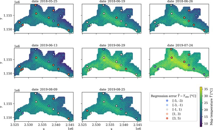
3522                                             M. Bosch et al.: A spatially explicit approach to simulate urban heat islands

depending on the satellite overpass time, the differences be-        decades, which has mostly occurred in the form of subur-
tween air temperature and LST can range from a few degrees           banization (Bosch et al., 2020).
(◦ C) up to tens of degrees (Jin and Dickinson, 2010; Sobrino           A notable geographic feature of Lausanne is its eleva-
et al., 2012), which calls for special caution when employing        tion difference of about 500 m between the lake shore at
satellite-derived LST data for the study of UHIs.                    372 m a.s.l. and the northeastern part of the agglomeration
   Although notable studies have explored the relationship           (see Fig. 1). The area is characterized by a continental tem-
between satellite-derived LST raster data and air tempera-           perate climate with mean annual temperatures of 10.9 ◦ C and
ture measurements to provide high-resolution insights into           mean annual precipitation of 1100 mm, and a dominating
the canopy-layer UHI (Fabrizi et al., 2010; Schwarz et al.,          vegetation of mixed broadleaf forest.
2012; Anniballe et al., 2014; Sheng et al., 2017; Shiflett et al.,
2017), they have mostly focused on finding statistical rela-         Spatial extent of the study
tionships between UHIs and the spatial distribution of terrain
features such as vegetation indices, without exploring how           In line with urban economics and regional sciences, many
the observed patterns relate to the biophysical mechanisms
                                                                     works rely on administrative boundaries to define the spatial
that explain the canopy-layer UHI. Such a limitation is im-
                                                                     extent of the study. However, the way in which boundaries
portant when models are used in simulations – for example,
                                                                     are constructed overlooks the characteristic scales at which
to examine the effect of urban planning scenarios on air tem-        landscape changes and environmental processes unfold, and
peratures. As part of the Integrated Valuation of Ecosystem          might thus lead to equivocal results (Liu et al., 2014; Oliveira
Services and Tradeoffs (InVEST) software, a suite of spatial         et al., 2014). Considering such issues, the spatial extent for
models to quantify and value the goods and services from
                                                                     this study was determined quantitatively by following the
nature that sustain and fulfill human life (Sharp et al., 2020),
                                                                     method employed in the Atlas of Urban Expansion (Angel
an urban cooling model has been developed following recent
                                                                     et al., 2012). The core idea is that a pixel is considered part
research on the effects of surface materials and vegetation          of the spatial extent depending on the proportion of built-
cover on UHIs (Phelan et al., 2015; Zardo et al., 2017). The         up pixels that surround it. In this study, a pixel is consid-
aim of the urban cooling model is to simulate the spatial dis-
                                                                     ered part of the spatial extent when more than 15 % of the
tribution of UHIs based on three key mechanisms, namely
                                                                     pixels that lay within a 500 m radius are built-up. Addition-
the shade provided by trees, the evapotranspiration of urban
                                                                     ally, in order to evaluate how temperatures change across the
vegetation and the albedo of the urban surface. In a prelim-
                                                                     urban–rural gradient, the spatial extent has been extended by
inary application of the model, Hamel et al. (2020) showed           a 1000 m buffer. The above procedure has been applied to the
its capability to represent the spatial pattern of nighttime air     rasterized land use and/or land cover (LULC) map by means
temperature of the 2003 heat waves in the Île-de-France re-
                                                                     of the Urban footprinter (Bosch, 2020b) Python library. The
gion.
                                                                     obtained spatial extent, displayed in Fig. 1, has a surface of
   The main objective of this study is to extend such pre-
                                                                     112.46 km2 .
liminary experiments by proposing a reusable computational
workflow to apply the InVEST urban cooling model to pre-
dict the spatial distribution of air temperature in a given study    2.2     Data
area. The validity of the simulated results is optimized by cal-
ibrating some key parameters to best fit a set of air temper-        2.2.1    Land use and/or land cover data
ature measurements from monitoring stations. Additionally,
the simulated spatial pattern of air temperature is compared         The LULC maps were obtained by rasterizing the vector
with one obtained using an alternative approach, namely a            geometries of the official cadastral survey of August 2019
spatial regression over features extracted from satellite data.      to a 10 m resolution. Such a dataset is provided and main-
                                                                     tained (i.e., updated weekly) by the cantonal administration
                                                                     of Vaud, and it features the whole spatial extent of the can-
2     Materials and methods                                          ton of Vaud (Association pour le Système d’information du
                                                                     Territoire Vaudois, 2018). The classification distinguishes 25
2.1    Study area                                                    LULC classes that are relevant to the urban, rural and wild
                                                                     landscapes encountered in Switzerland (Conference des Ser-
Situated at the western end of the Swiss Plateau and on              vices Cantonaux du Cadastre, 2011). Moreover, a 1 m binary
the shores of Lake Geneva, Lausanne is the fourth largest            tree canopy mask was derived from the SWISSIMAGE or-
Swiss urban agglomeration with 420 757 inhabitants as of             thomosaic (Federal Office of Topography, 2019), by means
January 2019 (Swiss Federal Statistical Office, 2018). As            of the DetecTree (Bosch, 2020a) Python library, which im-
the second most important student and research center in             plements the methods proposed by Yang et al. (2009). The
Switzerland (after Zurich), the urban agglomeration of Lau-          tree canopy mask of the spatial extent of the study is shown
sanne has experienced substantial growth during recent               in Fig. 1.

Geosci. Model Dev., 14, 3521–3537, 2021                                              https://doi.org/10.5194/gmd-14-3521-2021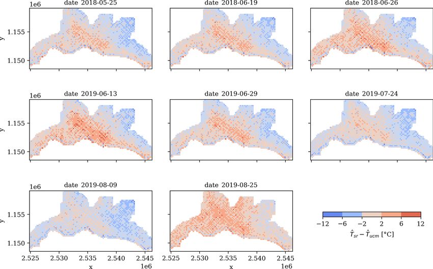
M. Bosch et al.: A spatially explicit approach to simulate urban heat islands                                                        3523

Figure 1. Study area. The upper left plot (A) shows the computed spatial extent (in orange) over the repartition of urban pixels (in black)
derived from the rasterized cadastral survey (Association pour le Système d’information du Territoire Vaudois, 2018). The upper right
plot (B) shows the locations of the air temperature measurement stations (see Appendix A2). The bottom row shows, for the computed spatial
extent of the study, (C) the tree canopy map derived from the SWISSIMAGE orthomosaic (Federal Office of Topography, 2019) and (D) the
altitude map derived from the free version of the digital height model of Switzerland (Federal Office of Topography, 2004). The basemap
of plots (A), (C) and (D) is based on the World Shaded Relief (© 2009 Esri). The basemap tiles of plot (B) have been provided by Stamen
Design (https://stamen.com, last access: 28 July 2020), under a Creative Commons BY 3.0 License (http://creativecommons.org/licenses/
by/3.0, last access: 28 July 2020), with data from OpenStreetMap (https://openstreetmap.org, last access: 28 July 2020, © OpenStreetMap
contributors 2021, distributed under a Creative Commons BY-SA License).

2.2.2   Elevation data                                                  tions operated by various governmental and research sources,
                                                                        which are shown in Fig. 1. The temporal resolution of the sta-
The elevation map for the study area, which is displayed in             tions ranges from 10 to 30 min. Given that the UHI effect in
Fig. 1, is extracted from the free version of the digital height        Switzerland reaches its maximal intensity around 21:00 CET
model of Switzerland (Federal Office of Topography, 2004),              (Burgstall, 2019), the remainder of this study evaluates it
provided at a 200 m resolution by the Federal Office of To-             based on the air temperature observations at the abovemen-
pography.                                                               tioned time.

2.2.3   Satellite data                                                  2.3   Simulation with the InVEST urban cooling model

The satellite dataset consists of the eight Landsat 8 images            The simulation of the spatial distribution of UHIs employs
in 2018 and 2019 that do not feature clouds over the study              the InVEST urban cooling model, version 3.8.0 (Sharp et al.,
area and comprise days on which the maximum observed air                2020), which is based on the heat mitigation provided by
temperature was over 25 ◦ C (see the list of selected image             shade, evapotranspiration and albedo. The main inputs are a
tiles in Appendix A1). Data from Landsat 7 were excluded                LULC raster map, a reference evapotranspiration raster and
because of the scan line corrector malfunction.                         a biophysical table containing model information of each
                                                                        LULC class of the map. Each row of the biophysical table
2.2.4   Air temperature data                                            represents a LULC class and features the following columns:

A dataset of consistent air temperature measurements in the                – lucode – the LULC class code as represented in the
study area was assembled by combining data from 11 sta-                      LULC raster map;

https://doi.org/10.5194/gmd-14-3521-2021                                                   Geosci. Model Dev., 14, 3521–3537, 2021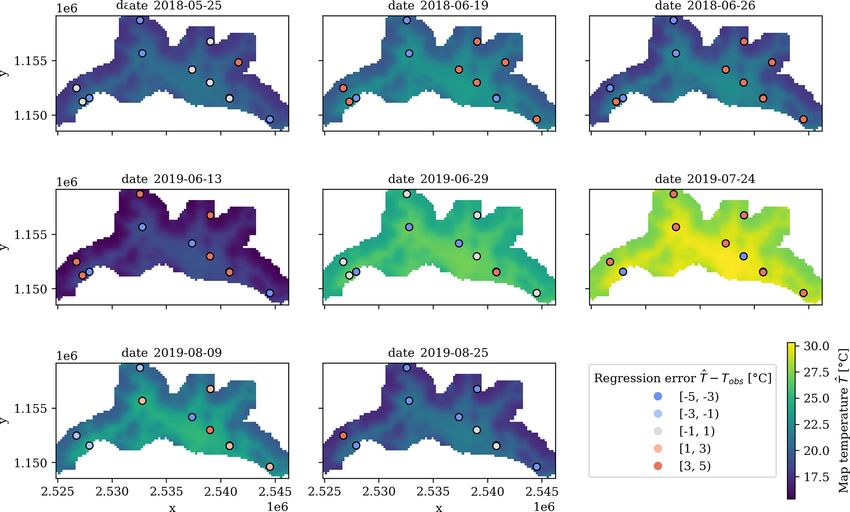
3524 M. Bosch et al.: A spatially explicit approach to simulate urban heat islands
– Shade – a value between zero and one representing the interest, and ETmax is the maximum evapotranspiration value
proportion of tree cover in such a LULC class; observed in the area of interest.
In line with the studies of Nistor and Porumb (2015), Nis-
– Kc – the evapotranspiration coefficient; tor et al. (2016) and Nistor (2016), the evapotranspiration co-
– Albedo – a value between zero and one representing efficients are attributed to each LULC class by distinguishing
the proportion of solar radiation directly reflected by the four cases, namely the crop coefficient for single crops for
LULC class; vegetation LULC classes, the water evaporation coefficient
for surface water, the rock and soil evaporation coefficient
– Green_area – whether the LULC class should be for bare soils and rocks, and evaporation coefficients for arti-
considered a green area or not; ficial LULC classes (e.g., urban areas). The evapotranspira-
– Building_intensity – a value between zero and tion coefficients attributed to the LULC classes of the Swiss
one representing the ratio between floor area and land cadastral survey are listed in Table A3.
area (for nighttime simulations). Following the recommendations of Allen et al. (1998), the
daily evapotranspiration ETref (in mm/d) was estimated for
2.3.1 Model description each pixel using the Hargreaves equation (Hargreaves and
Samani, 1985) as follows:
The data inputs described above are used to compute the
cooling capacity index, which is based on the physical mech- ETref = 0.0023 · (Tavg + 17.8) · (Tmax − Tmin )0.5 · Ra , (4)
anisms that contribute to cooling urban temperatures. More
where Tavg , Tmax and Tmin correspond to the average, maxi-
precisely, the cooling capacity index used in the InVEST
mum and minimum Tair (in ◦ C) of each day, respectively, and
urban cooling model builds upon the indices proposed by
Ra is the extraterrestrial radiation (in mm/d), which is esti-
Zardo et al. (2017), which are based on shading and evapo-
mated for the latitude of Lausanne (i.e., 46.519833◦ ) for each
transpiration, and extends them by adding a factor to account
date following the methods of Allen et al. (1998, Eq. 21). The
for the albedo. For each pixel i of the LULC raster map, the
temperature values of each day have been extracted from the
cooling capacity index is computed as follows:
inventory of gridded datasets provided by the Federal Of-
CCi = wS · Si + wAL · ALi + wET · ETIi , (1) fice of Meteorology and Climatology (MeteoSwiss), which
feature the minimum, average and maximum daily Tair for
where Si , ALi and ETIi represent the respective tree shading, the extent of the whole country at a resolution of 1 km.
albedo and evapotranspiration values of pixel i as defined in Such a dataset is obtained by interpolating 100 Tair stations
the biophysical table, and wS , wAL and wET represent the across Switzerland (including the MeteoSwiss Pully station
weights attributed to each respective component. The values in Fig. 1) based on nonlinear thermal profiles of major basins
of Si and ALi are retrieved from the biophysical table accord- and non-Euclidean distance weighting that accounts for ter-
ing to the LULC class k of the pixel i (see Appendix A3). rain effects (Frei, 2014).
The tree shading is computed by overlaying the binary tree In order to account for the cooling effect of large green
canopy mask with the rasterized LULC map so that for each spaces, the computed cooling capacity index of pixels that
LULC class k, the shade coefficient Sk corresponds to the are part of large green areas (> 2 ha) is adjusted as follows:
average proportion of tree cover over all the LULC pixels of
class k, as follows: green
X − d(i,j
d
)
CCi = gi · CCj · e cool , (5)
1 X j ∈i
Sk = xj . (2)
|k | j ∈
k where gi is one when the pixel i is a green area and zero oth-
erwise (as defined in the biophysical table), d(i, j ) is the dis-
Here, k is the set of pixels of the tree canopy mask whose
tance between pixels i and j , dcool is a parameter that defines
location corresponds to class k in the LULC raster, and xj
the distance over which a green space has a cooling effect,
is the value of pixel j of the tree canopy mask, i.e., one if j
and i is the set of pixels whose distance to i is lower than
corresponds to a tree and zero otherwise. The albedo coef-
dcool .
ficients are based on the local climate zone classification by
A heat mitigation (HM) index is then computed as follows:
Stewart and Oke (2012).
The evapotranspiration index ETI is computed as a nor-
CCi if i is part of a large green area
malized value of the potential evapotranspiration as follows: HMi = or CCi > CCi
green
(6)
green
CCi otherwise.
Kc · ETref
ETI = , (3)
ETmax
In order to simulate the spatial distribution of Tair , the model
where Kc is the evapotranspiration coefficient, ETref is the requires two additional inputs. The first is the rural reference
reference evapotranspiration raster for the period and area of temperature Tref , where the UHI effect is not observed, e.g.,
Geosci. Model Dev., 14, 3521–3537, 2021 https://doi.org/10.5194/gmd-14-3521-2021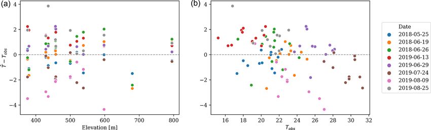
M. Bosch et al.: A spatially explicit approach to simulate urban heat islands                                                  3525

in the rural surroundings of the city. The second is the mag-         attributed to tree shading, albedo and evapotranspiration of
nitude of the UHI effect UHImax , namely the difference be-           wS = 0.6, wA = 0.2 and wET = 0.2, respectively. The num-
tween the rural reference temperature and the maximum Tair            ber of calibration iterations is set to 100.
observed in the city center. The two parameters are combined             Given that the Tref and UHImax parameters in this study
with HMi to compute the Ti for each pixel i of the study area         were obtained from observations from each simulated day,
as follows:                                                           metrics such as the mean absolute error (MAE) and the root
                                                                      mean squared error (RMSE) are effectively constrained to the
Tino mix = Tref + (1 − HMi ) · UHImax .                        (7)    [0, UHImax ] range, which affects the interpretation of these
                                                                      metrics. Therefore, in order to evaluate the ability of the In-
Finally, the Tair values of each pixel Tino mix are spatially aver-   VEST urban cooling model to spatially simulate UHIs, the
aged using a Gaussian function with a kernel radius r defined         coefficient of adjustment R 2 , MAE and RMSE of the cali-
by the user.                                                          brated model are compared with those computed in two ad-
                                                                      ditional experiments. The first experiment consisted of ran-
2.3.2   Calibration and evaluation of the model                       domly sampling the Tair values from a uniform distribution
                                                                      over the [Tref , UHImax ] range of each date. In the second ex-
To compare the InVEST urban cooling model with the spa-
                                                                      periment, the Tair values of each date were randomly sampled
tial regression based on satellite features, the urban cool-
                                                                      from a normal distribution with the mean and standard devia-
ing model is used to simulate the spatial distribution of Tair
                                                                      tion of the Tair measurements of the monitoring stations. For
for the same eight dates used to train the spatial regression
                                                                      both experiments, the three evaluation metrics are reported
model, i.e., the dates of the selected Landsat images. It is im-
                                                                      as their average over 10 runs.
plicitly assumed that no significant LULC changes have oc-
curred throughout study period (i.e., from May 2018 to Au-
gust 2019); therefore, all simulations depart from the same           2.4     Spatial regression of air temperature based on
LULC raster, i.e., the rasterized cadastral survey of the can-                satellite data
ton of Vaud as described above. Given the rugged terrain of
the study area, the Tref was set as the minimum average Tair          The spatial regression to predict Tair from features derived
observed among the monitoring stations, while UHImax was              from satellite data is performed over a raster dataset on a
set as the difference between the maximum average Tair ob-            per-pixel basis. A regression model is then trained to fit the
served among the monitoring stations and Tref . The values            observed Tair measurements by minimizing the error at the
of Tref and UHImax for the 8 d considered in this study are           pixels that correspond to the locations of the monitoring sta-
displayed in Fig. A1.                                                 tions.
   Although the documentation of the InVEST urban cooling                The regression operates in each pixel with the Tair as the
model (Sharp et al., 2020) provides some suggested values             target variable, and the elevation, the LST and the normalized
for several parameters of the model, their suitability depends        difference water index (NDWI) (Gao, 1996) as independent
strongly on the local geographic conditions of the study area.        variables. Additionally, to account for the influence of the
Therefore, calibration of the parameters is required in order         temperature and moisture surface conditions of each pixel,
to better understand how the physical mechanisms beyond               the LST and NDWI are spatially averaged over a series of cir-
the emergence of UHIs take place in the context of Lau-               cular neighborhoods with radii of 200, 400, 600 and 800 m,
sanne. Following the manual calibration approach drafted by           thereby reckoning eight supplementary features. Based on
Hamel et al. (2020), the target parameters are the weights at-        previous research on the sensitivity of the landscape pattern–
tributed to the tree shading (wS ), albedo (wA ) and evapotran-       UHI relationships to the spatial resolution (Weng et al., 2004;
spiration (wET ), the distance over which green spaces have           Song et al., 2014), the target resolution was set to 200 m.
a cooling effect (dcool ) and the Tair mixing radius (r). As an
additional contribution, this article implements an automated         2.4.1    Computation of satellite-derived features
calibrated procedure based on simulated annealing optimiza-
tion (Kirkpatrick et al., 1983) that aims at the minimization
                                                                      The estimation of the LST from Landsat 8 images followed
of the R 2 between the Tair values observed in the monitor-
                                                                      the methods of Avdan and Jovanovska (2016). On the one
ing stations and those predicted by the model1 . The param-
                                                                      hand, the data from the near-infrared (NIR) and red bands
eter values suggested in the documentation of the model are
                                                                      of Landsat 8 (i.e., bands 4 and 5, respectively) were used to
set as the initial state of the simulation annealing procedure,
                                                                      compute the normalized difference vegetation index (NDVI),
which corresponds to a Tair mixing radius of r = 500 m, a
                                                                      which was then used to estimate the ground emissivity (ελ ).
green area cooling distance of dcool = 100 m, and weights
                                                                      On the other hand, following the Landsat 8 Data Users Hand-
   1 The calibration module has been designed as a reusable           book (Zanter, 2015), the data from the thermal band of Land-
open-source Python package (see https://github.com/martibosch/        sat 8 (i.e., band 10) were first converted to top-of-atmosphere
invest-ucm-calibration; last access: 11 September 2020)               spectral radiance (Lλ ), from which brightness temperature

https://doi.org/10.5194/gmd-14-3521-2021                                                 Geosci. Model Dev., 14, 3521–3537, 2021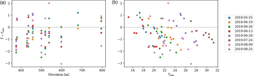
3526 M. Bosch et al.: A spatially explicit approach to simulate urban heat islands
(BT) was estimated (in ◦ C) as follows: and 0.580 ◦ C, and a respective RMSE of 1.508, 3.652 and
0.738 ◦ C. The coefficients suggest that SVM is not well
K2 suited for such a regression in this study area, whereas the
BT = − 273.15. (8)
ln((K1 /Lλ ) + 1) linear regression and random forest models obtain a very
strong fit – with the latter achieving the best performance.
Here, K1 and K2 are band-specific thermal conversion con-
Nevertheless, the average cross-validation scores suggest that
stants embedded in the Landsat image metadata. Finally, the
the linear regression (average score R 2 = 0.733) is more ro-
ground emissivity (ελ ) and the brightness temperature (BT)
bust to missing data and also less likely to over-fit the ob-
were used to compute the LST by inversion of Planck’s Law:
servations than the random forest regressor (average score
BT R 2 = 0.658). Thus, the remainder of the article only consid-
LST = , (9) ers the results obtained with a linear regression model trained
1 + λ · (BT/ρ) · ln(ελ )
with all of the samples.
where ρ = 1.438 × 10⁻² m K is a constant computed as a The importance of features of the chosen linear regres-
product of the Boltzmann constant and Planck’s constants sion model can be evaluated by means of an F test, as im-
divided by the velocity of the light, and λ = 10.895×10⁻⁹ is plemented in the statsmodels (Seabold and Perktold, 2010)
the average of the limiting wavelengths of the thermal band. Python library (see Table B1). With a significance level of
The NDWI is computed from the green and near-infrared p = 0.05, the results of the F test suggest that the most sig-
(NIR) bands of Landsat 8 (i.e., bands 3 and 5, respectively) nificant variable for the linear regression is the NDWI spa-
as follows: tially averaged over a 800, 600 and 400 m radius (in decreas-
ing order of significance). The following most significant
Xgreen − XNIR variable is the NDWI spatially averaged over a 200 m radius
NDWI = . (10)
Xgreen + XNIR (p = 0.071) and without spatial averaging (p = 0.231), and
the LST spatially averaged over a 400 m radius (p = 0.277).
2.4.2 Model selection and evaluation With a significance level of p = 0.420, the elevation does
not appear to be significant in this particular regression. The
Based on the work of Ho et al. (2014), three regression mod-
low significance obtained for the LST features in this study
els have been considered, namely a multiple linear regression
might be attributable to the large time lag between the ac-
model, a support-vector machine (SVM) model and a ran-
quisition time of the Landsat images (which ranges from
dom forest model. The accuracy of each regression model
11:15 to 11:23 CET) and the time of the Tair measurements
is assessed by means of a k-fold cross-validation procedure,
(i.e. 21:00 CET).
where the regression samples are first shuffled and parti-
The relationship between the predicted and the observed
tioned into three folds. For each fold k, a regression model
values is displayed in Fig. B1. The respective MAE and
is then trained using the other two folds, and it is validated
RMSE values of 1.198 and 1.508 ◦ C demonstrate a stronger
using the samples of the k fold. Finally, the model that shows
fit than the values of 1.82 and 2.31 ◦ C obtained in the study
the best validation score (i.e., the R 2 averaged over 10 repe-
of Ho et al. (2014) in Vancouver. The two plots in Fig. 2
titions of the k-fold procedure) is selected. Additionally, the
show the relationship between the elevation and Tobs of each
MAE and RMSE are computed in order to evaluate the devi-
sample and the regression errors. While there is no discern-
ations between the observed Tair and the predictions of each
able relationship regarding the elevation of the samples (i.e.,
model.
the elevation of the monitoring stations), the regression er-
The importance of each feature is also evaluated by com-
rors seem to be negatively correlated with Tobs . This pat-
puting its permutation importance (Breiman, 2001), namely
tern, which was also noted by Ho et al. (2014), indicates that
the average decrease in the regression accuracy when a fea-
high-temperature samples are systematically underestimated
ture is randomly shuffled. The training of the regression mod-
by the regression model, whereas low-temperature samples
els, the cross-validation and the permutation feature impor-
are consistently overestimated.
tance described above have been implemented by means of
The series of predicted Tair maps for the eight dates as well
the Scikit-learn library (Pedregosa et al., 2011).
as the prediction errors at the locations of the monitoring sta-
tions are displayed in Fig. 3. While the range of temperatures
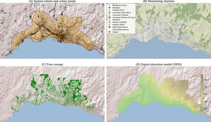
3 Results exhibits important differences throughout the dates, the spa-
tial distribution of Tair is seemingly consistent. The highest
3.1 Spatial regression of air temperature based on temperatures persistently occur in the most urbanized areas,
satellite data whereas the lowest temperatures take place at higher eleva-
tions located in the east and northeast of the map. Finally,
When including all of the samples, the R 2 for the linear there seems to be no discernable pattern in space nor time
regression, SVM and random forest are 0.832, 0.014 and regarding the prediction errors at the monitoring stations.
0.960, respectively, with a respective MAE of 1.198, 2.671
Geosci. Model Dev., 14, 3521–3537, 2021 https://doi.org/10.5194/gmd-14-3521-2021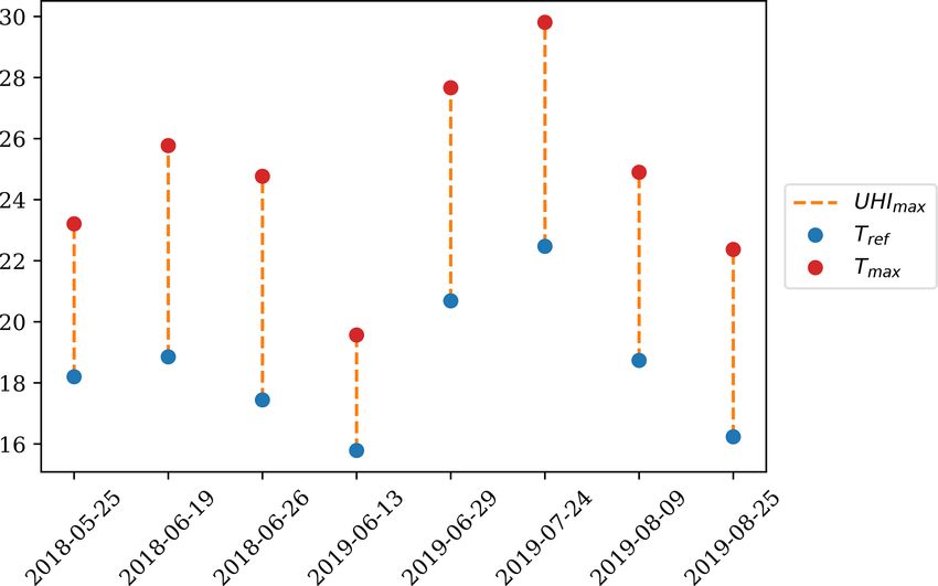
M. Bosch et al.: A spatially explicit approach to simulate urban heat islands                                                           3527

Figure 2. Scatterplot of the spatial regression residuals (y axis) against the elevation of the monitoring station (x axis of panel a) and the
observed Tair (x axis of panel b), colored by the sample date. See Appendix B.

Figure 3. Maps of the Tair predicted by the spatial regression for the eight dates. The points in the map correspond to the location of the
monitoring stations and are colored according to the regression errors.

3.2   Simulation with the InVEST urban cooling model                     tively; these values suggest better model performance than
                                                                         randomly sampling from the station measurements. Random
                                                                         sampling from the station measurements yields a respective
The parameters of the model that result in the best fit of
                                                                         R 2 , MAE and RMSE of 0.573, 1.947 and 2.405 ◦ C when
the station measurements are a Tair mixing radius of r =
                                                                         sampling from a uniform distribution and 0.550, 1.952 and
236.02 m, a green area cooling distance of dcool = 89.21 m,
                                                                         2.468 ◦ C when sampling from a normal distribution. Further-
and weights attributed to tree shading, albedo and evapo-
                                                                         more, the values of R 2 , MAE and RMSE obtained with the
transpiration of wS = 0.59, wA = 0.24 and wET = 0.17, re-
                                                                         calibrated parameters reveal a stronger fit than the spatial re-
spectively (see Appendix B). The R 2 , MAE and RMSE of
                                                                         gression reported above.
the calibrated model are 0.903, 0.955 and 1.144 ◦ C, respec-

https://doi.org/10.5194/gmd-14-3521-2021                                                     Geosci. Model Dev., 14, 3521–3537, 2021
3528 M. Bosch et al.: A spatially explicit approach to simulate urban heat islands
The relationship between the Tair values at the monitoring 4 Discussion
stations simulated with the calibrated parameters and the ac-
tual observed measurements is shown in Fig. B2. The differ-
ences between Tair simulated at the monitoring stations and The results obtained in this study suggest that both the spa-
the observed values are plotted against the elevation and the tial regression based on satellite data and the InVEST urban
observed temperatures (Tobs ) in Fig. 4. The pattern of such cooling model are capable of predicting the spatial distribu-
relationships is very similar to that observed in the spatial re- tion of air temperature with a large degree of statistical de-
gression. Conversely, there is no clear relationship between termination. Furthermore, the fact that a similar spatial pat-
the prediction error of the urban cooling model and eleva- tern is predicted by both models suggests that the biophys-
tion. Moreover, the prediction errors exhibit a negative cor- ical mechanisms embedded in the urban cooling model are
relation with the observed temperature, denoting a system- well represented. If that is the case, the urban cooling model
atic tendency to both underestimate high temperatures and presents two central advantages with respect to the spatial
overestimate low temperatures – with the former being more regression.
prominent in this case, as is noticeable from the asymmetry The first advantage is that, in contrast to regressions and
of the y axis in Fig. 4. black-box approaches, the biophysical mechanisms that drive
The simulated Tair maps for the eight dates and the predic- the emergence of UHIs are represented explicitly; this allows
tion errors at the monitoring stations are shown in Fig. 5. As for a physical interpretation of the parameters of the model.
in the spatial regression, the temperature ranges show impor- For example, in a comparative study of the relationship be-
tant differences across dates, yet the same spatial pattern of tween the LST and the spatial configuration of trees in Balti-
Tair persists. The simulated distribution of Tair shows its high- more and Sacramento, Zhou et al. (2017) suggested that the
est values in the center of Lausanne and along the most ur- distinctive results observed in each city might be related to
banized (and hence less forested) zones along the main trans- how the shading of trees and evapotranspiration contribute
portation axes, whereas the lowest temperatures are found in differently to urban cooling in the climatic context of each
the forested areas located in the eastern and western extremes city. More precisely, the abovementioned study suggested
of the upper half of the study area. that in the dry climate of Sacramento, large patches of trees
ameliorate the efficiency of the evapotranspiration, whereas
3.3 Model comparison the gains from the tree shading are likely more important in
the humid climate of Baltimore. The urban cooling model
A comparison of the maps predicted by the spatial regres- provides a suitable means to quantitatively address such mat-
sion and the urban cooling model is displayed in Fig. 6. ters – i.e., by calibrating the model in the two cities, we can
In line with the temporal consistency of the spatial patterns explore the weights obtained for each factor to support such a
predicted by the respective two approaches, the comparison hypothesis. In the case study of Lausanne reported above, the
maps also show a spatial distribution of Tair that persists weight attributed to the tree shading (wS = 0.59) is higher
throughout the dates. Such a spatial pattern is strongly remi- than that attributed to the evapotranspiration (wET = 0.17).
niscent of the elevation maps (see Fig. 1 above) and reflects This is consistent with the local climatic conditions being
the fact that elevation is explicitly considered in the spatial more similar in Lausanne and Baltimore than in Sacramento;
regression but not in the urban cooling model. The over- however, the weights obtained in this study might be partly
all distribution of the Tair pixel differences between the two determined by the initial solution provided. Nonetheless, to
approaches follows a normal distribution that ranges from further understand this issue, validation and calibration of the
−9.620 to 11.929 ◦ C (reflecting the lower and higher tem- InVEST urban cooling model in a broader variety of cities is
peratures predicted in the spatial regression, respectively), required. Overall, the way in which the calibrated parame-
which is a considerably large range when compared with the ters differ from the recommendations in the documentation
small overall MAE and RMSE of both approaches. Nonethe- of the model are in consonance with the particular character-
less, the way in which the histogram is centered around 0 ◦ C istics of Lausanne. More precisely, the smaller mixing radius
suggests that the differences between the two approaches fol- and cooling distances are consistent with the uneven relief of
low no particular correlation other than the spatial regression the study area.
predicting more extreme Tair values, which is not surprising The second major advantage of the urban cooling model
considering that the range of Tair is systematically bounded is that once the model is calibrated for a given city, it can be
in the urban cooling model by the Tref and UHImax parame- used to evaluate synthetic scenarios, such as those stemming
ters. from master plans, urbanization prospects or the like, and to
spatially design solutions. This kind of spatially explicit eval-
uation of the impacts of alternative scenarios on ecosystem
services is in fact one of the central purposes of the InVEST
suite of models (Tallis and Polasky, 2009). Statistical models
like the spatial regression are not well suited to such a pur-
Geosci. Model Dev., 14, 3521–3537, 2021 https://doi.org/10.5194/gmd-14-3521-2021M. Bosch et al.: A spatially explicit approach to simulate urban heat islands 3529 Figure 4. Scatterplot of the differences between the Tair simulated by the InVEST urban cooling model and the values observed at the monitoring stations (y axis) against the elevation of the monitoring station (x axis of panel a) and the observed Tobs (x axis of panel b), colored by the sample date. Figure 5. Maps of the Tair simulated by the InVEST urban cooling model for the eight dates. The points on the map correspond to the location of the monitoring stations and are colored according to the simulation errors. pose, as they rely on features, such as the LST, that are hard the air is mixed and the cooling effects of large green spaces. to obtain other than empirically. In complex terrains such as the Lausanne agglomeration, The approach proposed in this article is nevertheless sub- models with uniform weighting of space show considerable ject to some limitations that merit thoughtful consideration. deviations from the observed distribution of air temperature On the one hand, as acknowledged in its user guide (Sharp (Frei, 2014). On the other hand, the relationship between the et al., 2020), the design of the InVEST urban cooling model calibration parameters and the resulting R 2 is likely to de- presents a number of limitations, the most relevant to this fine a complex optimization landscape with multiple local study being the simplified and homogeneous way in which optima. As a metaheuristic that strongly depends on random https://doi.org/10.5194/gmd-14-3521-2021 Geosci. Model Dev., 14, 3521–3537, 2021
3530                                             M. Bosch et al.: A spatially explicit approach to simulate urban heat islands

Figure 6. Maps comparing the difference between the Tair predicted by the spatial regression T̂sr and the InVEST urban cooling model T̂ucm
for the eight dates (see Appendix B).

decisions, the simulated annealing procedure is susceptible            high-resolution LST datasets, is one of the main reasons why
to convergence to local optima, arbitrarily leading to differ-         most UHI studies have focused on the latter (Jin and Dick-
ent solutions in each run. A sensitivity analysis of the param-        inson, 2010; Zhou et al., 2019). As illustrated in this article,
eters of the urban cooling model as undertaken preliminar-             spatial regressions based on remote sensing features such as
ily by Hamel et al. (2020) for the Île-de-France region could          the LST and NDWI do not necessarily replicate the air tem-
serve as a basis to improve the simulated annealing proce-             perature measurements better than biophysical models such
dure by careful design of an appropriate neighborhood search           as the InVEST urban cooling model. Therefore, improving
and annealing schedule. Finally, the approach of the present           the spatial density of the monitoring network becomes im-
study is based on observations at the moment of maximal                perative for further enlightenment with respect to the UHI
UHI intensity (i.e., 21:00 CET in Switzerland); however, the           phenomena.
factors that influence UHIs are likely to operate differently
across the diurnal UHI cycle. In fact, several studies point
to distinct relationships between the spatial patterns of veg-         5   Conclusions
etation and daytime and nighttime UHIs (Anniballe et al.,
2014; Sheng et al., 2017; Shiflett et al., 2017; Hamel et al.,         The present article presents a spatially explicit approach
2020). Considering the nature of the implications of UHIs,             to simulate UHIs with the InVEST urban cooling model,
e.g., energy consumption, work productivity or human health            which is based on three biophysical mechanisms, namely
(Koppe et al., 2004; Santamouris et al., 2015; Zander et al.,          tree shade, evapotranspiration and albedo. The proposed ap-
2015), a sound understanding of the full diurnal UHI cycle             proach shows how LULC and air temperature data can be
becomes crucial towards the design of robust solutions.                combined to calibrate the parameters of the model to best
   Nevertheless, the limitations on how the urban cooling              fit measurements from monitoring stations by means of an
model represents the spatial air mixing and the cooling ef-            automated procedure. The simulations performed for the ur-
fects of green spaces seem hard to overcome with the cur-              ban agglomeration of Lausanne show that the InVEST urban
rent spatial sparsity of monitoring stations. Such a major             cooling model can outperform spatial regressions based on
shortcoming, which contrasts with the growing availability of          satellite-derived features such as LST, NDWI and elevation.

Geosci. Model Dev., 14, 3521–3537, 2021                                                  https://doi.org/10.5194/gmd-14-3521-2021
M. Bosch et al.: A spatially explicit approach to simulate urban heat islands                                     3531

The way in which both approaches consistently predict the
highest temperatures in the most urbanized parts of the ag-
glomeration suggests that the enhancement of green infras-
tructure can be an effective heat mitigation strategy; however,
further exploration in other climatic contexts is required to
fully understand this issue. To that end, the reusability of the
computational workflow paves the way for further applica-
tion of the urban cooling model to a broad variety of cities,
which can serve to improve the understanding of the UHI
phenomena and support the design of heat mitigation strate-
gies.

https://doi.org/10.5194/gmd-14-3521-2021                                        Geosci. Model Dev., 14, 3521–3537, 2021
3532                                           M. Bosch et al.: A spatially explicit approach to simulate urban heat islands

Appendix A: Data                                                  A4   Reference temperatures and UHI magnitude

A1     Landsat tiles

The list of product identifiers for the Landsat image tiles are
available as a comma-separated value (CSV) file at https:
//zenodo.org/record/4384675/files/landsat-tiles.csv (last ac-
cess: 13 July 2020).

A2     Monitoring stations

The list of monitoring stations with their operator and
their elevation in meters above sea level is available
as a CSV file at https://zenodo.org/record/4384675/files/
station-tair.csv (last access: 13 July 2020). The operators are
Agrometeo, the Federal Roads Office (ASTRA), the Federal
Office for the Environment (BAFU), the general directorate
for the environment of the canton of Vaud (DGE), and the          Figure A1. Reference temperatures Tref (i.e., minimum Tair at
Federal Institute of Forest, Snow and Landscape Research          21:00 CET among the monitoring stations) and magnitude of the
(WSL) (Rebetez et al., 2018).                                     UHI UHImax (i.e., difference between Tref and the maximum Tair
                                                                  at 21:00 CET among the monitoring stations) for the eight dates
A3     Biophysical table                                          considered in this study.

The biophysical table used in the computational workflow is
available as a CSV file at https://zenodo.org/record/4384675/
files/biophysical-table.csv (last access 13 July 2020). The
crop and water coefficients are based on Allen et al. (1998),
whereas rock, soil and urban coefficients are derived from the
results of Grimmond and Oke (1999) in the city of Chicago.
Given that the evapotranspiration of the vegetation and crops
is subject to seasonal changes in temperate zones such as
Switzerland (Allen et al., 1998), the values correspond to
the mid-season estimation (June to August) in Nistor (2016).
The albedo values are based on the work of Stewart and Oke
(2012). The shade column, which represents the proportion
of tree cover of each LULC class, has been computed with
a high-resolution tree canopy map of Lausanne and is, there-
fore, specific to the study area. Rows with a dash (–) in the
shade column denote that the corresponding LULC class is
not present in the study area.

Geosci. Model Dev., 14, 3521–3537, 2021                                           https://doi.org/10.5194/gmd-14-3521-2021
M. Bosch et al.: A spatially explicit approach to simulate urban heat islands 3533
Appendix B: Results
B1 Tables
Table B1. F test of variable significance of the linear regression.
Feature Coefficient SE t P > |t| [0.025 0.975]
const 1.1760 3.369 0.349 0.728 −5.534 7.886
lst_0 0.4944 0.584 0.846 0.400 −0.669 1.658
ndwi_0 −6.1852 5.127 −1.206 0.231 −16.396 4.026
lst_200 −0.3267 0.885 −0.369 0.713 −2.089 1.435
ndwi_200 −28.5531 15.581 −1.833 0.071 −59.585 2.479
lst_400 −1.9332 1.765 −1.095 0.277 −5.449 1.583
ndwi_400 124.2456 46.749 2.658 0.010 31.138 217.353
lst_600 1.0526 2.963 0.355 0.723 −4.849 6.955
ndwi_600 −156.7220 55.931 −2.802 0.006 −268.119 −45.325
lst_800 1.7306 1.685 1.027 0.308 −1.626 5.087
ndwi_800 85.4412 22.732 3.759 0.000 40.167 130.715
elev −0.0026 0.003 −0.810 0.420 −0.009 0.004
B2 Figures
Figure B1. Scatterplot of the Tair predicted by the linear regression model trained with all of the samples (y axis) versus the observed
measurements (x axis).
https://doi.org/10.5194/gmd-14-3521-2021 Geosci. Model Dev., 14, 3521–3537, 20213534 M. Bosch et al.: A spatially explicit approach to simulate urban heat islands Figure B2. Scatterplot of the Tair values simulated with the InVEST urban cooling model (y axis) versus the observed measurements (x axis). Geosci. Model Dev., 14, 3521–3537, 2021 https://doi.org/10.5194/gmd-14-3521-2021
M. Bosch et al.: A spatially explicit approach to simulate urban heat islands                                                            3535

Code availability. The code materials used in this article are            Acknowledgements. This research has been supported by the École
available at https://doi.org/10.5281/zenodo.4916285 (Bosch, 2021)         Polytechnique Fédérale de Lausanne (EPFL). The authors grate-
and are maintained in a GitHub repository at https://github.com/          fully thank Yves Kazemi and Martin Schlaepfer for their help with
martibosch/lausanne-heat-islands (last access: 22 December 2020).         the study design, Rémi Jaligot for his careful review of the paper
   The code for the spatial regression of air temperature from            before submission, Bethanna Jackson for editing the article as well
satellite data is available as a Jupyter Notebook (IPYNB)                 as Daniel Rodrigues and Rubianca Benavidez for reviewing it.
at        https://github.com/martibosch/lausanne-heat-islands/blob/
gmd-published/notebooks/spatial-regression.ipynb (last access:
9 June 2021).                                                             Financial support. This research has been supported by the École
   The code of the spatial simulation of air temperature with the         Polytechnique Fédérale de Lausanne (EPFL).
InVEST urban cooling model is available as a Jupyter Notebook
(IPYNB) at https://github.com/martibosch/lausanne-heat-islands/
blob/gmd-published/notebooks/invest-urban-cooling-model.ipynb             Review statement. This paper was edited by Bethanna Jackson and
(last access: 9 June 2021).                                               reviewed by Daniel Rodrigues and Rubianca Benavidez.
   The code used for the comparison of the spatial regression and
simulation of air temperature is available as a Jupyter Notebook
(IPYNB) at https://github.com/martibosch/lausanne-heat-islands/
blob/gmd-published/notebooks/comparison.ipynb (last access:               References
9 June 2021).
                                                                          Allen, R. G., Pereira, L. S., Raes, D., and Smith, M.: Crop
                                                                            evapotranspiration-Guidelines for computing crop water require-
Data availability. The source files for the biophysical table, list of      ments – FAO Irrigation and drainage paper 56, Fao, Rome, 300,
landsat tiles, reference evapotranspiration, station locations and sta-     ISBN 92-5-104219-5, 1998.
tion temperature measurements for the reference dates can be found        Angel, S., Sheppard, S., Civco, D. L., Buckley, R., Chabaeva, A.,
in a dedicated archive at https://zenodo.org/record/4384675 (last           Gitlin, L., Kraley, A., Parent, J., and Perlin, M.: The dynamics of
access: 13 July 2020). The reference evapotranspiration raster is           global urban expansion, Citeseer, Transport and Urban Develop-
obtained using the minimum, average and maximum temperature                 ment Department of The World Bank, Washington D.C., 2005.
datasets of the copyrighted Spatial Climate Analyses of MeteoSwiss        Angel, S., Blei, A. M., Civco, D. L., and Parent, J.: Atlas of ur-
(Frei, 2014). The temperature observations correspond to monitor-           ban expansion, Lincoln Institute of Land Policy Cambridge, MA,
ing stations operated by Agrometeo, the Federal Roads Office (AS-           2012.
TRA), the Federal Office for the Environment (BAFU), the gen-             Anniballe, R., Bonafoni, S., and Pichierri, M.: Spatial and temporal
eral directorate for the environment of the Canton of Vaud (DGE),           trends of the surface and air heat island over Milan using MODIS
and the Federal Institute of Forest, Snow and Landscape Research            data, Remote Sens. Environ., 150, 163–171, 2014.
(WSL) (Rebetez et al., 2018).                                             Arnfield, A. J.: Two decades of urban climate research: a review of
   The source files for the spatial extent of the study area and the        turbulence, exchanges of energy and water, and the urban heat
respective land use and/or land cover raster map can be found at            island, Int. J. Climatol., 23, 1–26, 2003.
a dedicated archive at https://doi.org/10.5281/zenodo.4311544 (last       Association pour le Système d’information du Territoire Vaudois:
access: 15 July 2020; Bosch, 2020c). The obtained extent is based           Structure es données cadastrales au format SHAPE (MD.01-
on the official cadastral survey of the canton of Vaud whose exclu-         MO-VD), available at: https://www.asitvd.ch/md/508 (last ac-
sive owner is the Canton of Vaud, with the use conditions disclosed         cess: 3 September 2019), 2018 (in French).
in the norm OIT 8401.                                                     Avdan, U. and Jovanovska, G.: Algorithm for automated mapping
   The tree canopy map can be found at a dedicated archive at               of land surface temperature using LANDSAT 8 satellite data, J.
https://doi.org/10.5281/zenodo.4310112 (Bosch, 2020d). The map              Sensors, 2016, 1480307, 2016.
has been obtained based on the SWISSIMAGE 2016 aerial imagery             Bosch, M.: DetecTree: Tree detection from aerial im-
dataset.                                                                    agery in Python, J. Open Source Softw., 5, 2172,
                                                                            https://doi.org/10.21105/joss.02172, 2020a.
                                                                          Bosch, M.: Urban footprinter: a convolution-based ap-
                                                                            proach to detect urban extents from raster data, Zenodo,
Author contributions. MB and ML designed the study and con-
                                                                            https://doi.org/10.5281/zenodo.3699310, 2020b.
ducted the analysis with technical input from PH and RPR and over-
                                                                          Bosch, M.: Lausanne agglomeration extent [Data set], Zenodo,
all supervision from JC and SJ. MB developed the code and wrote
                                                                            https://doi.org/10.5281/zenodo.4311544, 2020c.
the paper. All authors provided comments and contributed to the
                                                                          Bosch, M.: Lausanne tree canopy [Data set], Zenodo,
final version of the paper.
                                                                            https://doi.org/10.5281/zenodo.4310112, 2020d.
                                                                          Bosch,       M.:       martibosch/lausanne-heat-islands:       GMD
                                                                            published       (Version    gmd-published)       [code],   Zenodo,
Competing interests. The authors declare that they have no conflict         https://doi.org/10.5281/zenodo.4916285, 2021.
of interest.                                                              Bosch, M., Jaligot, R., and Chenal, J.: Spatiotemporal patterns of
                                                                            urbanization in three Swiss urban agglomerations: insights from
                                                                            landscape metrics, growth modes and fractal analysis, Landscape
                                                                            Ecol., 35, 879–891, 2020.

https://doi.org/10.5194/gmd-14-3521-2021                                                      Geosci. Model Dev., 14, 3521–3537, 2021
3536 M. Bosch et al.: A spatially explicit approach to simulate urban heat islands
Breiman, L.: Random forests, Mach. Learning, 45, 5–32, 2001. Liu, Z., He, C., Zhou, Y., and Wu, J.: How much of the world’s
Burgstall, A.: Representing the Urban Heat Island Effect in Fu- land has been urbanized, really? A hierarchical framework for
ture Climates, Scientific Report MeteoSwiss No. 105, Zürich, avoiding confusion, Landscape Ecol., 29, 763–771, 2014.
Switzerland, 2019. Nistor, M.-M.: Mapping evapotranspiration coefficients in the Paris
Clinton, N. and Gong, P.: MODIS detected surface urban heat is- metropolitan area, GEOREVIEW Scientific Annals of Ştefan cel
lands and sinks: Global locations and controls, Remote Sens. En- Mare University of Suceava, Geography Series, 26, 138–153,
viron., 134, 294–304, 2013. 2016.
Conference des Services Cantonaux du Cadastre: De- Nistor, M.-M. and Porumb, G. C. G.: How to compute the land
gré de spécification en mensuration officielle – Couche cover evapotranspiration at regional scale? A spatial approach
d’information de la couverture du sol, available at: of Emilia-Romagna region, GEOREVIEW: Scientific Annals of
https://www.cadastre.ch/content/cadastre-internet/fr/manual-av/ Stefan cel Mare University of Suceava, Geography Series, 25,
publication/guidline.download/cadastre-internet/fr/documents/ 38–53, 2015.
av-richtlinien/Richtlinie-Detaillierungsgrad-BB-fr.pdf (last Nistor, M.-M., Gualtieri, A. F., Cheval, S., Dezsi, Ş., and Boţan,
access: 26 Februrary 2020), 2011 (in French). V. E.: Climate change effects on crop evapotranspiration in the
Fabrizi, R., Bonafoni, S., and Biondi, R.: Satellite and ground-based Carpathian Region from 1961 to 2010, Meteorol. Appl., 23, 462–
sensors for the urban heat island analysis in the city of Rome, 469, 2016.
Remote Sens., 2, 1400–1415, 2010. Oke, T. R.: City size and the urban heat island, Atmos. Environ., 7,
Federal Office of Topography: DHM25/200 m The free version of 769–779, 1973.
the digital height model of Switzerland, available at: https://shop. Oke, T. R.: The energetic basis of the urban heat island, Q. J. Roy.
swisstopo.admin.ch/en/products/height_models/dhm25200 (last Meteor. Soc., 108, 1–24, 1982.
access: 21 March 2020), 2004. Oliveira, E. A., Andrade Jr, J. S., and Makse, H. A.: Large cities are
Federal Office of Topography: SWISSIMAGE La mosaïque less green, Sci. Rep., 4, 1–13, 2014.
d’ortophotos de la Suisse, available at: https://shop.swisstopo. Pedregosa, F., Varoquaux, G., Gramfort, A., Michel, V., Thirion, B.,
admin.ch/fr/products/images/ortho_images/SWISSIMAGE (last Grisel, O., Blondel, M., Prettenhofer, P., Weiss, R., Dubourg, V.,
access: 3 March 2020), 2019 (in French). Vanderplas, J., Passos, A., Cournapeau, D., Burcher, M., Perrot,
Frei, C.: Interpolation of temperature in a mountainous region using M. and Duchesnay, É.: Scikit-learn: Machine learning in Python,
nonlinear profiles and non-Euclidean distances, Int. J. Climatol., J. Mach. Learn. Res., 12, 2825–2830, 2011.
34, 1585–1605, 2014. Phelan, P. E., Kaloush, K., Miner, M., Golden, J., Phelan, B.,
Gao, B.-C.: NDWI – A normalized difference water index for re- Silva III, H., and Taylor, R. A.: Urban heat island: mechanisms,
mote sensing of vegetation liquid water from space, Remote implications, and possible remedies, Annu. Rev. Environ. Re-
Sens. Environ., 58, 257–266, 1996. sour., 40, 285–307, 2015.
Grimm, N. B., Faeth, S. H., Golubiewski, N. E., Redman, C. L., Wu, Rebetez, M., von Arx, G., Gessler, A., Pannatier, E. G., Innes,
J., Bai, X., and Briggs, J. M.: Global change and the ecology of J. L., Jakob, P., Jetel, M., Kube, M., Nötzli, M., Schaub, M.,
cities, Science, 319, 756–760, 2008. Schmitt, M., Sutter, F., Thimonier, A., Waldner, P., and Haeni,
Grimmond, S. and Oke, T.: Evapotranspiration rates in urban areas, M.: Meteorological data series from Swiss long-term forest
in: Proceedings of the Impacts of Urban Growth on Surface Wa- ecosystem research plots since 1997, Ann. Forest Sci., 75, 41,
ter and Groundwater Quality HS5, 235–243, International Asso- https://doi.org/10.1007/s13595-018-0709-7, 2018.
ciation of Hydrological Sciences Publications, Birmingham, UK, Santamouris, M., Cartalis, C., Synnefa, A., and Kolokotsa, D.: On
1999. the impact of urban heat island and global warming on the power
Hamel, P., Tardieu, L., Lemonsu, A., de Munck, C., and Viguié, demand and electricity consumption of buildings – A review, En-
V.: Co-développement du module rafraîchissement offert par la erg. Buildings, 98, 119–124, 2015.
végétation de l’outil InVEST, Report submited to the Agence Schwarz, N., Lautenbach, S., and Seppelt, R.: Exploring indicators
de l’environnement et de la Maîtrise de l’energie (ADEME), for quantifying surface urban heat islands of European cities with
IDEFSE reports, Paris, France, 2020. MODIS land surface temperatures, Remote Sens. Environ., 115,
Hargreaves, G. H. and Samani, Z. A.: Reference crop evapotranspi- 3175–3186, 2011.
ration from temperature, Appl. Eng. Agric., 1, 96–99, 1985. Schwarz, N., Schlink, U., Franck, U., and Großmann, K.: Relation-
Ho, H. C., Knudby, A., Sirovyak, P., Xu, Y., Hodul, M., and Hen- ship of land surface and air temperatures and its implications for
derson, S. B.: Mapping maximum urban air temperature on hot quantifying urban heat island indicators – An application for the
summer days, Remote Sens. Environ., 154, 38–45, 2014. city of Leipzig (Germany), Ecol. Ind., 18, 693–704, 2012.
Jin, M. and Dickinson, R. E.: Land surface skin temperature clima- Seabold, S. and Perktold, J.: statsmodels: Econometric and statisti-
tology: Benefitting from the strengths of satellite observations, cal modeling with python, in: 9th Python in Science Conference,
Environ. Res. Lett., 5, 044004, https://doi.org/10.1088/1748- 28 June–3 July, Austin, Texas, 2010.
9326/5/4/044004, 2010. Sharp, R., Tallis, H., Ricketts, T., Guerry, A., Wood, S., Chaplin-
Kirkpatrick, S., Gelatt, C. D., and Vecchi, M. P.: Optimization by Kramer, R., Nelson, E., Ennaanay, D., Wolny, S., Olwero, N.,
simulated annealing, Science, 220, 671–680, 1983. Vigerstol, K., Pennington, D., Mendoza, G., Aukema, J., Foster,
Koppe, C., Sari Kovats, R., Jendritzky, G., and Menne, B.: Heat- J., Forrest, J., Cameron, D., Arkema, K., Lonsdorf, E., Kennedy,
waves: risks and responses, Tech. rep., WHO Regional Office C., Verutes, G., Kim, C. K., Guannel, G., Papenfus, M., Toft, J.,
for Europe, Copenhagen, 2004. Marsik, M., Bernhardt, J., Griffin, R., Glowinski, K., Chaumont,
N., Perelman, A., Lacayo, M. Mandle, L., Hamel, P., Vogl, A. L.,
Geosci. Model Dev., 14, 3521–3537, 2021 https://doi.org/10.5194/gmd-14-3521-2021You can also read