A PYTHON-ENHANCED URBAN LAND SURFACE MODEL SUPY (SUEWS IN PYTHON, V2019.2): DEVELOPMENT, DEPLOYMENT AND DEMONSTRATION - GMD
←
→
Page content transcription
If your browser does not render page correctly, please read the page content below
Geosci. Model Dev., 12, 2781–2795, 2019
https://doi.org/10.5194/gmd-12-2781-2019
© Author(s) 2019. This work is distributed under
the Creative Commons Attribution 4.0 License.

A Python-enhanced urban land surface model SuPy (SUEWS in
Python, v2019.2): development, deployment and demonstration
Ting Sun and Sue Grimmond
Department of Meteorology, University of Reading, Reading, RG6 6BB, UK

Correspondence: Ting Sun (ting.sun@reading.ac.uk) and Sue Grimmond (c.s.grimmond@reading.ac.uk)

Received: 10 February 2019 – Discussion started: 21 March 2019
Revised: 12 June 2019 – Accepted: 18 June 2019 – Published: 9 July 2019

Abstract. Accurate and agile modelling of cities weather,         Ward and Grimmond, 2017; Zhao et al., 2014), pedestrian
climate, hydrology and air quality is essential for integrated    level meteorology to diagnose thermal comfort (Bar et al.,
urban services. The Surface Urban Energy and Water bal-           2011; Erell et al., 2013; Krayenhoff et al., 2018; Sun et al.,
ance Scheme (SUEWS) is a state-of-the-art widely used ur-         2016; Tan et al., 2009), or ambient radiation and wind condi-
ban land surface model (ULSM) which simulates urban–              tions to assist building design (Chen, 2004; Jentsch et al.,
atmospheric interactions by quantifying the energy, water         2013; B. Li et al., 2015; Lindberg and Grimmond, 2011;
and mass fluxes. Using SUEWS as the computation ker-              Reinhart and Cerezo Davila, 2016; Santamouris et al., 2001).
nel, SuPy (SUEWS in Python) uses a Python-based data              To obtain such information, accurate and agile modelling ca-
stack to streamline the pre-processing, computation and post-     pacity of the urban weather and climate are essential.
processing that are involved in the common modelling-                Urban land surface models (ULSMs) are widely used to
centred urban climate studies. This paper documents the de-       simulate urban–atmosphere interactions by quantifying the
velopment of SuPy, including the SUEWS interface modifi-          energy, water and mass fluxes between the surface and urban
cation, F2PY (Fortran to Python) configuration and Python         atmosphere (Best and Grimmond, 2015; Chen et al., 2011;
front-end implementation. In addition, the deployment of          Wang et al., 2012). These models require information on ur-
SuPy via PyPI (Python Package Index) is introduced along          ban morphology (e.g. heights, spacings of buildings, etc.)
with the automated workflow for cross-platform compilation.       and anthropogenic dynamics (e.g. building-operation-related
This makes SuPy available for all mainstream operating sys-       heat release, emissions of heat by traffic) to be included.
tems (Windows, Linux and macOS). Three online tutorials              One widely used and tested ULSM, the Surface Urban En-
in Jupyter Notebook are provided to users of different lev-       ergy and Water balance Scheme (SUEWS; Table 1), requires
els to become familiar with SuPy urban climate modelling.         basic meteorological data and surface information to charac-
The SuPy package represents a significant enhancement that        terize essential urban features (i.e. urban surface heterogene-
supports existing and new model applications, reproducibil-       ity and anthropogenic dynamics). SUEWS enables long-term
ity and enhanced functionality.                                   urban climate simulations without specialized computing fa-
                                                                  cilities (Järvi et al., 2011, 2014; Ward et al., 2016). SUEWS
                                                                  is regularly enhanced (Grimmond et al., 1991, 1986; Grim-
                                                                  mond and Oke, 1991; Järvi et al., 2011, 2014, 2019; Of-
1   Introduction                                                  ferle et al., 2003; Ward et al., 2016) and tested in cities un-
                                                                  der a range of climates worldwide (Table 1). Although oper-
Cities need to be resilient to weather, climate, hydrological     ationally simple and scientifically robust, SUEWS still re-
and air quality hazards given their large and ever-increasing     quires some skill for application (e.g. computing environ-
populations (Baklanov et al., 2018). One prerequisite to          ment setup, parameter configuration), which may limit up-
building resilience is information at various spatio-temporal     take for broader applications in urban planning and design.
scales, e.g. to understand energy partitioning over urban sur-
faces (D. Li et al., 2015; Sun et al., 2017; Wang et al., 2015;

Published by Copernicus Publications on behalf of the European Geosciences Union.
2782                                         T. Sun and S. Grimmond: A Python-enhanced urban land surface model SuPy

Table 1. Recent studies using SUEWS. D&E – development and evaluation. n/a – not applicable

  Topic                                                                          City                     Reference
  Impact of haze on the urban water balance                                      Beijing, China           Kokkonen et al. (2019)
  CO2 emissions module: D&E                                                      Helsinki, Finland        Järvi et al. (2019)
  Impact of precipitation forcing on the urban water balance                     London, UK               Ward et al. (2018)
  Impacts of anthropogenic heat and irrigation on surface energy balance         Shanghai, China          Ao et al. (2018)
  Sensitivity of SUEWS to forcing variables                                      Vancouver, Canada        Kokkonen et al. (2018)
                                                                                 London, UK
  SUEWS a core processor of the UMEP system                                      (n/a)                    Lindberg et al. (2018)
  Impacts of changes in surface cover, human behaviour and climate on en-        London, UK               Ward and Grimmond (2017)
  ergy partitioning
  Offline evaluation of SUEWS driven by WRF output                               Porto, Portugal          Rafael et al. (2017)
  Implications of warming to cold climate cities                                 High-latitude cities     Järvi et al. (2017)
  Evaluation in Singapore and comparison with other urban land surface           Singapore                Demuzere et al. (2017)
  models
  Evaluation in four cities with different climates                              Dublin, Ireland          Alexander et al. (2016)
                                                                                 Hamburg, Germany
                                                                                 Melbourne, Australia
                                                                                 Phoenix, USA
  Evaluation of SUEWS in two UK cities                                           London, UK               Ward et al. (2016)
                                                                                 Swindon, UK
  Evaluation of radiation flux in Shanghai                                       Shanghai, China          Ao et al. (2016)
  Boundary layer modelling and coupling with SUEWS                               Sacramento, USA          Onomura et al. (2015)
  Evaluation with Local Climate Zone information as surface characteristics      Dublin, Ireland          Alexander et al. (2015)
  Model inter-comparison for sensible and latent heat fluxes                     Helsinki, Finland        Karsisto et al. (2015)
  Snow melt model D&E                                                            Helsinki, Finland        Järvi et al. (2014)
                                                                                 Montreal, Canada
  SUEWS D&E                                                                      Vancouver, Canada        Järvi et al. (2011)
                                                                                 Los Angeles, USA

   Reproducibility and open science principles are increas-           2     Development
ingly important (Peng, 2011). Although climate scientists
by convention publish detailed model configurations used in           The following are considered within the design process of
their research, minor inconsistencies or lack of transparency         SuPy:
of code often hampers efforts to reproduce simulation re-
sults. In addition, new users may lack prerequisite knowl-                 1. Data preparation. Climate simulations typically require
edge in low-level compilation and scripting to undertake ini-                 extensive pre-processing of data (loading input data, re-
tial model runs and interpretation of simulation results (Lin,                formatting to conform with standards, etc.) and post-
2012).                                                                        processing (conversion of output, graphical and carto-
   Today Python is used extensively by the atmospheric sci-                   graphic plotting, etc.). Python has a vast array of util-
ences community for data analyses and numerical mod-                          ities to support this; notably, NumPy (the fundamen-
elling (Lin, 2012; Perkel, 2015) thanks to its simplicity and                 tal package for scientific computing with Python, https:
the large scientific Python ecosystem (e.g. PyData com-                       //www.numpy.org, last access: 12 June 2019) and pan-
munity: https://pydata.org, last access: 12 June 2019). Re-                   das (a tabular-format-centred data analysis tool) are two
cent Python-based endeavours include global climate system                    cornerstone libraries in Python-based scientific comput-
models (Monteiro et al., 2018), stochastic geological models                  ing.
(de la Varga et al., 2019) and hydrological models (Hamman
                                                                           2. Performance. Python, as a scripting language, has
et al., 2018) to cite just a few.
                                                                              poorer performance than compiled languages (e.g. C,
   In this paper, we present a Python-enhanced urban cli-
                                                                              Fortran; Kouatchou, 2018). For this reason, Fortran is
mate system based on the popular Fortran-coded SUEWS
                                                                              used extensively for weather and climate-related soft-
– SuPy (SUEWS in Python). The development of SuPy
                                                                              ware (e.g. WRF – Skamarock and Klemp, 2008; GFDL
(Sect. 2), the essential workflow in its cross-platform deploy-
                                                                              AM3 – Donner et al., 2011; etc.). Therefore, by using
ment (Sect. 3), and three demonstration tutorials for users of
                                                                              different languages their individual strengths can be uti-
different levels (Sect. 4) are presented.
                                                                              lized.

Geosci. Model Dev., 12, 2781–2795, 2019                                                    www.geosci-model-dev.net/12/2781/2019/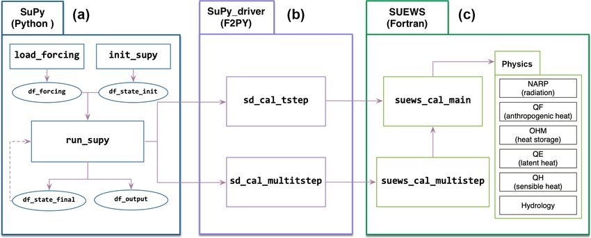
T. Sun and S. Grimmond: A Python-enhanced urban land surface model SuPy 2783
3. Cross-platform ability. Given the range of computer en- useful in flexible manipulation of SuPy runtime behaviours
vironments, it is important that software can be easily (application in Sect. 4.3), while the latter has much better
used across operating systems with ease. Python and performance because of the much lower computational over-
Fortran are both easily used on most operating systems. heads with the F2PY wrapper. Therefore, sd_cal_multitstep
However, for performance reasons as noted, it is prefer- is the default executer in run_supy, the SuPy core proces-
able to have a compiled back end for intensive simula- sor performing simulations, for regular runs without runtime
tions, where platform-specific compilations are manda- manipulation.
tory. Thus, we adopt the Microsoft Azure Pipelines to In addition to run_supy, SuPy uses pandas DataFrame
allow for a cross-platform ability for SuPy (Sect. 3.1). as the central data structure to simplify the pre- and
post-processing as required by the original SUEWS.
4. Extendibility. It is desirable, possibly even essential, for
The overall data structures used in SuPy are described
the scientific model to interact with other models and
in the documentation (https://supy.readthedocs.io/en/latest/
data sources to extend the overall capacity and to ex-
data-structure/supy-io.html, last access: 12 June 2019). The
plore questions related to urban climate beyond the cli-
pre-processor is designed to load existing SUEWS input
mate science.
files, which consists of the following (Appendix A):
To address these four considerations, SuPy’s architecture
uses Python’s data processing and Fortran’s computational 1. init_supy. This loads surface characteristics (e.g.
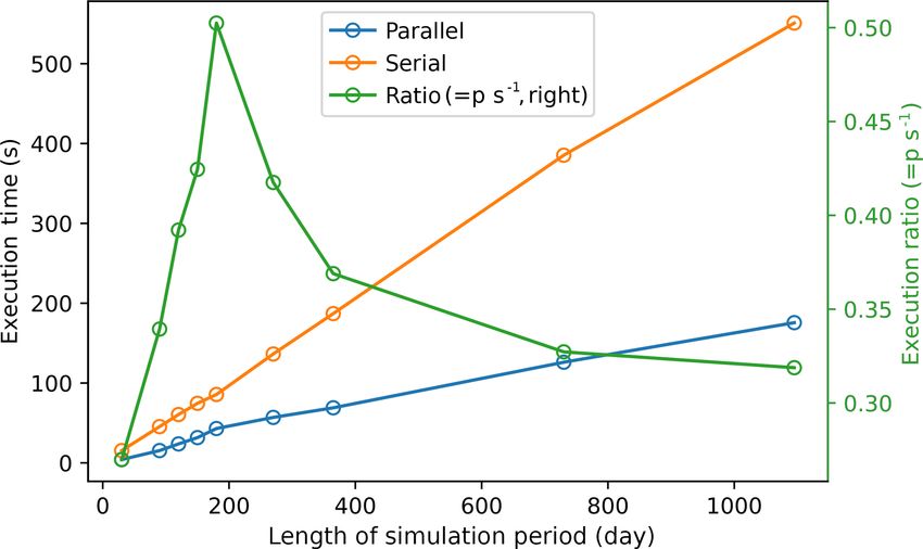
efficiency. SuPy consists of three parts (Fig. 1): albedo, emissivity, land cover fractions; full
details given in the SUEWS documentation:
1. SuPy. A Python-based front-end processor based on the https://suews-docs.readthedocs.io/en/latest/input_
pandas DataFrame with functionality for data analysis files/SUEWS_SiteInfo/SUEWS_SiteInfo.html,
and simulation management (Appendix A). last access: 12 June 2019) and model configu-
2. SuPy_driver. Calculation kernel compiled by F2PY rations (e.g. stability correction option chosen;
(Fortran to Python, part of the NumPy package) (Peter- https://suews-docs.readthedocs.io/en/latest/input_
son, 2009) to facilitate the transfer of SUEWS’ Fortran files/RunControl/RunControl.html, last access:
modelling ability to Python and guarantee the computa- 12 June 2019). The data go into df_state_init (a pan-
tional performance. das DataFrame; https://supy.readthedocs.io/en/latest/
data-structure/df_state.html, last access: 12 June 2019).
3. SUEWS. A Fortran-coded local-scale urban land sur- Two auxiliary json files are used with the look-
face model of moderate complexity that can simulate up hierarchies for loading this information from
the urban surface energy balance in combination with SUEWS library files (https://suews-docs.readthedocs.
the complete urban hydrological cycle, considering irri- io/en/latest/input_files/input_files.html, last access:
gation and runoff processes (Grimmond and Oke, 1986, 12 June 2019) in a consistent file-code-variable way.
1991; Järvi et al., 2011, 2014; Offerle et al., 2003; Ward
et al., 2016). 2. load_forcing. Meteorological and other external
Development of SuPy (Sun, 2019) started with SUEWS forcing information are loaded into df_forcing (a
v2017b (Ward and Grimmond, 2017). SUEWS has three dis- pandas DataFrame; https://supy.readthedocs.io/en/
tinct groups of subroutines: model physics, input and out- latest/data-structure/df_forcing.html, last access:
put (I/O). To help generalize coupling, the use of Fortran 12 June 2019) to drive the SuPy simulations with
modules to pass variables and parameters has been reduced time-step size inferred from its DatetimeIndex (i.e. the
and there has been a return to further use of Fortran subrou- freq attribute). SUEWS should be run at short time
tine arguments with explicitly stated intent (e.g. in, out). The steps (e.g. 5 min) as precipitation or irrigation runoff
modified physics subroutines are called from two subrou- from impervious surfaces becomes too large if the
tines, suews_cal_main and suews_cal_multistep (Fig. 1a), water arrives as one large hourly (or longer) amount
depending on the model time step (single or multi). This (Grimmond and Oke, 1991; Ward et al., 2018). As
structure constitutes the SUEWS v2018c calculation ker- such, load_forcing is implemented with the ability
nel (Fig. 1a) and enables efficient communication between to downscale the raw forcing data to finer time steps
SUEWS and other models (e.g. WRF) through an explicit (5 min by default). The temporal resolution of raw
and unified interface. forcing data can be between 5 and 360 min, with
The SUEWS kernel (v2018c) is compiled by F2PY to gen- 30–60 min being the most common.
erate the Python-compliant SuPy_driver package. Using the
two subroutines allows better computational performance.
The SuPy_driver calls the two subroutines depending on Detailed guidance is provided in SUEWS documen-
time-step simulation type: single- (sd_cal_tstep) or multi- tation for preparing input files (https://suews-docs.
time-step mode (sd_cal_multitstep, Fig. 1b). The former is readthedocs.io/en/latest/input_files/input_files.html, last
www.geosci-model-dev.net/12/2781/2019/ Geosci. Model Dev., 12, 2781–2795, 2019
2784                                         T. Sun and S. Grimmond: A Python-enhanced urban land surface model SuPy

Figure 1. SuPy’s three major components (left to right): (a) SuPy, a Python-based front-end processor; (b) SuPy_driver, the calculation
kernel compiled by F2PY; (c) SUEWS, a Fortran-coded local-scale urban land surface model. Note that not all physics schemes are listed.

access: 12 June 2019) and in the Urban Multi-scale Envi-              3    Deployment
ronmental Predictor (UMEP) documentation (https://umep-
docs.readthedocs.io/en/latest/pre-processor/SUEWS         Pre-        To achieve cross-platform compatibility, SuPy has two parts:
pare.html, last access: 12 June 2019). SUEWS uses
multiple ASCII text and namelist files (https://suews-docs.               1. SuPy_driver (calculation kernel): the F2PY generated
readthedocs.io/en/latest/input_files/input_files.html,     last              binaries of SUEWS are platform-dependent because of
access: 12 June 2019), and UMEP (Lindberg et al., 2018)                      compilation being necessary for assurance of perfor-
provides a QGIS/Python interface that is designed to aid                     mance.
the derivation of the spatial parameters from geodata. As
SuPy can use the files prepared by the other two approaches,              2. SuPy (front-end processor): this platform-independent
existing SUEWS files are usable via the init_supy and                        Python code allows rapid iteration in functionality
load_forcing functions for SuPy.                                             enhancement and bug fixing thanks to the powerful
   For new users without experience of other versions, a                     ecosystem of Python utilities.
helper function, load_SampleData, is provided to get the
sample input DataFrames (i.e. df_state_init and df_forcing)
                                                                      As software compilation can be frustrating and/or prone
ready to run simulations. Once users understand the
                                                                      to operator errors, this procedure is automated using
SUEWS/SuPy variables, the sample DataFrames provide a
                                                                      two online services: Microsoft Azure Pipeline (https:
template to work with to meet their next specific needs. Ex-
                                                                      //azure.microsoft.com/en-us/services/devops/pipelines/,
amples using the sample datasets are provided as tutorials
                                                                      last access: 12 June 2019) for continuous integration
(Sect. 4).
                                                                      (CI) and PyPI (Python Package Index; https://pypi.org,
   As the F2PY-compiled kernel, SuPy_driver, relies on
                                                                      last access: 12 June 2019) for distribution. Mi-
NumPy ndarray for data input and output, two SuPy post-
                                                                      crosoft Azure Pipeline has good cross-platform support
processors, pack_state and pack_output, are embedded in
                                                                      (https://docs.microsoft.com/en-gb/azure/devops/pipelines/
run_supy to pack the (1) ndarray output of model final
                                                                      agents/agents?view=azure-devops, last access: 1 July 2019)
states into df_state_final (a pandas DataFrame; https://supy.
                                                                      and easy connection with code repositories (e.g. GitHub:
readthedocs.io/en/latest/data-structure/df_state.html, last ac-
                                                                      https://github.com, last access: 12 June 2019; Bitbucket:
cess: 12 June 2019) and (2) simulation results to df_output
                                                                      https://bitbucket.com, last access: 12 June 2019) and sup-
(a pandas DataFrame; https://supy.readthedocs.io/en/latest/
                                                                      ports automated compilation for different platforms. The
data-structure/df_output.html, last access: 12 June 2019).
                                                                      Azure Pipeline build workflow permits a variety of func-
To facilitate reuse of model runs (e.g. for model spin-up),
                                                                      tionalities to facilitate compilation and publishing to other
df_state_final has the same data structure as df_state_init
                                                                      online services (e.g. PyPI, GitHub pages, etc.). Currently,
(dashed line, SuPy panel, Fig. 1a).
                                                                      this is set up for three major platforms (Windows, macOS
                                                                      and Linux) with three Python 3 configurations (3.5, 3.6 and
                                                                      3.7) to conduct automated compilation of SuPy back-end
                                                                      files: SUEWS binaries and SuPy_driver, the product of
                                                                      which is directly pushed to PyPI and released in real time.

Geosci. Model Dev., 12, 2781–2795, 2019                                                 www.geosci-model-dev.net/12/2781/2019/
T. Sun and S. Grimmond: A Python-enhanced urban land surface model SuPy 2785
To build the SuPy_driver two crucial steps to allow cross- 4 Demonstration: SuPy tutorials
platform deployment (full details refer to configuration file
setup.py in SuPy_driver) are the following. To familiarize users with SuPy urban climate modelling
and to demonstrate the functionality of SuPy, we provide
1. Static linking: to eliminate the issue of missing dy- three tutorials (Table 2, access at https://supy.readthedocs.
namic libraries, the calculation kernels are pre-built us- io/en/latest/tutorial/tutorial.html, last access: 12 June 2019)
ing static linking and therefore run directly after down- in Jupyter notebooks (https://jupyter.org/, last access:
loading. 12 June 2019).
They can run in browsers (e.g. desktop, tablet) either
2. manylinux tagging: given the many Linux distribu- by local configuration or on remote servers with pre-
tions and their different runtime libraries that often set environments (e.g. Google Colaboratory, https://colab.
require distribution-specific compilation, we use the research.google.com, last access: 12 June 2019; Microsoft
manylinux docker image (for details refer to https: Azure Notebooks, https://notebooks.azure.com, last access:
//github.com/pypa/manylinux) to compile SuPy_driver. 12 June 2019). As Jupyter notebooks allow source code to
be incorporated with detailed notes, users can organize their
In addition to the cross-platform compilation, to guarantee analyses (Shen, 2014). Jupyter notebooks can be installed
delivery quality we perform automatic code tests of four pre- with pip on any desktop/server system and open .ipynb note-
set configurations for every build: book files locally (Listing 2). We note that running SuPy in
browsers is not implemented by SuPy per se but allowed by
1. Connectivity between SuPy and SuPy_driver: checks if the Jupyter environment where Python 3 is supported. The
the front-end processor and back-end calculation core reason for running SuPy (and many other python applica-
can communicate with correct input and output. tions) on mobile devices (e.g. mobile phone, tablet) is sim-
ple: working seamlessly across different devices is a natural
2. Success in single-time-step mode: checks SuPy can pro- need.
duce correct simulation results in the single-time-step
mode.
3. Success in multi-time-step mode: checks SuPy can pro-
Listing 2. Command line code for installing Jupyter Notebook
duce correct simulation results in the multi-time-step
with pip and open an existing local .ipynb notebook file (i.e.
mode and does a quick benchmark of computation
path_to_your_notebook).
speed.
These are made available to SUEWS by calling
4. Compare simulation results between single- and multi- the load_SampleData function. This produces pandas
time-steps modes: checks SuPy can produce identical DataFrames with the initial model state (df_state_init) and
simulation results as designed. the forcing variables (df_forcing). These are used in all three
tutorials.
All build and test output is logged in detail (see all logs
here: https://dev.azure.com/sunt05/SuPy/_build, last access: 4.1 SuPy quick-start
12 June 2019) and the results are reported to developers in
real time. This feature is used for all code and underpins a In this tutorial, we demonstrate the key steps in using SuPy to
commitment for timely support to SuPy development. undertake the core task to simulate energy and water balance
The Python Package Index (PyPI: https://pypi.org, last ac- in an urban context using SUEWS. Here the runs are for a
cess: 12 June 2019) is the official third-party software repos- central London area in 2012.
itory for Python. As it is supported by the pip toolchain it The urban surface energy balance (SEB) can be expressed
provides Python users easy worldwide access to packages as
and frees Python developers from maintaining indexing and
distribution servers. By using the PyPI channel, SuPy can be Q∗ + QF = QH + QE + 1QS , (1)
easily installed by users with a one-line input in a command where the flux densities (W m−2 ) are Q∗ net all-wave radia-
line tool on any desktop/server system (Listing 1). tion, QF anthropogenic heat, QH turbulent sensible heat, QE
latent heat and 1QS the net storage heat flux. Through QE ,
the SEB characteristics can be linked to the water balance:
Listing 1. Command line code for SuPy installation using pip. Note P + I = E + R + 1S, (2)
64-bit Python 3.5+ is required for SuPy installation. where each term is a depth of water per unit of time
(e.g. mm d−1 ). P is precipitation, I irrigation, E evapotran-
www.geosci-model-dev.net/12/2781/2019/ Geosci. Model Dev., 12, 2781–2795, 20192786 T. Sun and S. Grimmond: A Python-enhanced urban land surface model SuPy
Table 2. Three SuPy tutorials. Note that the website links redirect to online Jupyter notebooks for SuPy simulation without any configuration
by users.
Name Aim Audience
Quick-start SuPy Essential workflow to conduct New users, students
(https://mybinder.org/v2/gh/sunt05/SuPy/master?filepath= SuPy simulations
docs/source/tutorial/quick-start.ipynb,
last access: 1 July 2019)
Impact studies using SuPy in parallel mode Impacts on urban climate from Urban climate researchers with
(https://mybinder.org/v2/gh/sunt05/SuPy/master?filepath= varying surface characteristics experience in land surface sim-
docs/source/tutorial/impact-studies-parallel.ipynb, and forcing conditions ulations
last access: 1 July 2019)
Interaction between SuPy and external models Couple SuPy and external mod- Model developers with back-
(https://mybinder.org/v2/gh/sunt05/SuPy/master?filepath= els for agile development ground in climate modelling
docs/source/tutorial/external-interaction.ipynb,
last access: 1 July 2019)
Table 3. Default settings in the sample dataset provided with SuPy for (a) physics scheme and (b) basic site characteristics. For full
SuPy variable setting details refer to the online documentation: https://supy.readthedocs.io/en/latest/data-structure/df_state.html (last access:
12 June 2019).
(a) Basic site characteristics SuPy parameter (unit) Value
Land cover fractions: building, paved, sfr (–) [0.43, 0.38, 0.001, 0.019, 0.029, 0.001, 0.14]
evergreen tree, deciduous tree, grass,
bare soil and water
Building height bldgh (m) 22.0
Evergreen tree height evetreeh (m) 13.1
Deciduous tree height dectreeh (m) 13.1
(b) Physics scheme Code Remark
Radiation radiationmethod 3 Net all-wave radiation modelled with incoming long-
wave radiation modelled using air temperature and rel-
ative humidity (Loridan et al., 2011)
Heat storage storageheatmethod 1 OHM model (Grimmond et al., 1991)
Anthropogenic heat emissionsmethod 2 Anthropogenic heat model responding to temperature,
population density, time of day and day of week (Järvi
et al., 2011)
Snow snowuse 1 Snow module to model snowpack and related thermal
and hydrological dynamics (Järvi et al., 2014)
Roughness length for momentum roughlenmommethod 2 Momentum roughness length determined using Grim-
mond and Oke (1999)
Roughness length for heat roughlenheatmethod 2 Thermal roughness length determined using Kawai et
al. (2009)
Atmospheric stability stabilitymethod 3 Atmospheric stability correction function (Campbell
and Norman, 1998)
Geosci. Model Dev., 12, 2781–2795, 2019 www.geosci-model-dev.net/12/2781/2019/T. Sun and S. Grimmond: A Python-enhanced urban land surface model SuPy 2787
Figure 2. Intra-annual (2012) variation in forcing variables in the sample dataset (from top to bottom): incoming solar radiation, air tem-
perature, relative humidity, air pressure, wind speed and rainfall in central London All variables are hourly averages except for total hourly
rainfall (source of data: Kotthaus and Grimmond, 2014; gap filled: Ward et al., 2016).
spiration (= QE /Lv where Lv is the latent heat of vaporiza-
tion), R runoff and 1S the net change in water storage.
The fundamental steps to use SuPy after the software en-
vironment has been installed (see Listings 1, 2) are (1) load
input, (2) run a simulation and (3) examine the results. With
everything ready, three lines of python code are needed.
SuPy is run by calling run_supy after df_state_init and Listing 3. Python code for a minimal SuPy simulation with com-
df_forcing have been loaded. After the simulation the two ments (green).
DataFrames provide major SUEWS outputs (df_output) and
the model state (df_state_final) at the end of the run. The
latter can be used as initial conditions for other SuPy runs.
The post-processing uses pandas functions to resample,
plot and write out the model output. The default output
www.geosci-model-dev.net/12/2781/2019/ Geosci. Model Dev., 12, 2781–2795, 20192788 T. Sun and S. Grimmond: A Python-enhanced urban land surface model SuPy
DataFrame of 5 min resolution can be upscaled to the month be expected that the maximum and mean values of T2 are
for an overview of intra-annual dynamics of surface energy greatly reduced as they are directly influenced by the altered
and water balances (Fig. 3). net solar radiation, while impacts on the minimum T2 might
This workflow using SuPy for urban climate modelling be expected to be minimal.
can be easily adapted to existing SUEWS tutorials under the In this tutorial we demonstrate some starting cases rather
UMEP framework (https://tutorial-docs.readthedocs.io, last than a complete research cycle. Notably, limitations are im-
access: 12 June 2019) by replacing the conventional SUEWS posed in the configuration used (e.g. length of the model run,
binary executable with the python SuPy package. Given the spin-up period, feedbacks permitted) and thus the relations
central role of Python in the UMEP framework, it is expected shown should be interpreted with caution.
the adoption of SuPy will further streamline the workflows To explore changes in atmospheric forcing, the DataFrame
for urban climate simulations in UMEP. df_forcing is modified. In this example, we investigate the
impact of increased local-scale (constant flux layer) air tem-
4.2 Impacts of the urban area on local climate perature Ta on the near-surface air temperature T2 . Air tem-
perature Ta is increased over 24 runs from 0 ◦ C (no change)
A major application of urban climate models is to study the to +2 ◦ C. The upper limit (+2 ◦ C) represents a highly pos-
impacts on urban climate from design scenarios that change sible average global warming scenario for the near future
surface characteristics or the climate (atmospheric forcing). (IPCC, 2014). The SuPy simulations are conducted from Jan-
In this tutorial both scenario types are explored: we provide uary to July 2012 and July data are analysed. The T2 results
one example of modification of albedo for surface character- indicate the increased Ta has different impacts on the T2 met-
istics, while another of air temperature alteration for climate rics (minimum, mean and maximum) but all increase linearly
conditions. with Ta . The maximum T2 has the stronger response com-
Technically, this requires several configuration files to pared to the other metrics (Fig. 6).
be prepared for a suite of independent model runs. These This tutorial demonstrates the simplicity of using SuPy to
could be run consecutively (i.e. no interactions between runs conduct impact studies of both surface characteristics and
are needed) or in parallel, so-called “embarrassingly paral- background climates. These can be easily adapted by users
lel computation” (Bailey et al., 1991), with multiple inde- to their specific application interests. Thus, as various effects
pendent runs with sufficient CPUs. In this tutorial, we first are combined the net impacts becomes more realistic.
demonstrate how SuPy can be easily set up to efficiently
complete multiple simulations in parallel. 4.3 Interaction between SuPy and external models
We use dask (https://dask.org, last access: 12 June 2019)
to parallelize the SuPy simulations given its close coherence SUEWS can be coupled to other models that provide or re-
with NumPy and pandas, in particular its almost identical quire forcing data using the SuPy single-time-step running
DataFrame interfaces as pandas. Specifically, we use the ap- mode (Sect. 2). We demonstrate this feature with a simple
ply method of dask.DataFrame to improve the simulation online anthropogenic heat flux model.
performance by distributing the SuPy computations across Anthropogenic heat flux (QF ) is an additional term to the
different configurations. Compared with the serial mode, the surface energy balance in urban areas associated with human
dask-based parallel mode takes only ∼ 30 % of the execution activities (Gabey et al., 2018; Grimmond, 1992; Nie et al.,
time of the serial mode for simulations longer than 1000 d 2014, 2016; Sailor, 2011). In most cities, the largest emission
for 12 grids (Fig. 4). The parallel configuration for running source is from buildings (Hamilton et al., 2009; Iamarino
SuPy, run_supy_mgrids, is then used in the following two et al., 2011; Sailor, 2011) and is highly dependent on out-
cases for more efficient parallel simulations. door ambient air temperature. For demonstration purposes
To explore the effect of changes to surface properties, the we have created a very simple model instead of using the
DataFrame df_state_init needs to be modified. The surface SUEWS QF (Järvi et al., 2011) with feedback from outdoor
albedo of different materials impacts the outgoing shortwave air temperature (Fig. 7). The simple QF model considers only
(solar) radiation and thus the surface energy balance fluxes building heating and cooling:
and other atmospheric variables. Modifying roof albedo has
been suggested extensively as a method to cool urban areas (T2 − TC ) × CB , T2 > TC ;
(e.g. Santamouris et al., 2011; Li et al., 2014; Ramamurthy et QF = (TH − T2 ) × HB , T2 < TH ; (3)
al., 2015). In the example, we conduct simulations from Jan-
QF0 ,
uary 2012 to July 2012 with the first 6 months as the spin-up
period. The building roof albedo is incrementally increased where TC (TH ) is the cooling (heating) threshold tempera-
from 0.1 to 0.8 (e.g. a change from a very dark to a very ture of buildings, CB (HB ) is the building cooling (heating)
light surface). The near-surface temperature T2 , an indica- rate and QF 0 is the baseline anthropogenic heat. The param-
tor of thermal state at pedestrian level, is analysed using the eters used are TC (TH ) set as 20 ◦ C (10 ◦ C), CB (HB ) set as
monthly maximum, mean and minimum (Fig. 5). It would 1.5 W m−2 K−1 (3 W m−2 K−1 ) and QF0 is set as 0 W m−2 ,
Geosci. Model Dev., 12, 2781–2795, 2019 www.geosci-model-dev.net/12/2781/2019/T. Sun and S. Grimmond: A Python-enhanced urban land surface model SuPy 2789 Figure 3. SuPy simulated monthly (a) surface energy and (b) water balance for London 2012. Assuming no irrigation. Figure 4. Comparison of execution times (seconds) between serial and parallel modes when 12 grids are simulated for different periods Figure 5. Impacts of increasing building roof albedo α (from 0.1) (days): 30, 90, 120, 150, 180, 270, 365, 730 and 1095. Simulations on near-surface temperature T2 considering monthly maximum, performed with macOS 10.14.3 running on 2.9 GHz Intel Core i9 mean and minimum temperatures at 2 m for July 2012 based on with 32 GB memory. The model configuration is the same as Quick- 5 min output. start SuPy (Table 2). implying other building activities (e.g. lightning, water heat- tion using SuPy coupled is performed for London in 2012. ing, computers) are zero and therefore do not change the tem- The data analysed are a summer (July) and a winter (De- perature or change with temperature. cember) month. Initially, QF is 0 W m−2 and the T2 is deter- The coupling between the simple QF model and SuPy is mined and used to determine QF [1] , which in turn modifies done via the low-level function suews_cal_tstep, which is an T2[1] and therefore modifies QF [2] and the diagnosed T2[2] . interface function in charge of communications between the Results indicate a positive feedback, as QF is increases T2 is SuPy front end and the calculation kernel. By setting SuPy to elevated but with different magnitudes (Fig. 8). Of particular receive external QF as forcing, at each time step, the simple note is the positive-feedback loop under warm air temper- QF model is driven by the SuPy output T2 and provides SuPy atures: the anthropogenic heat emissions increase, which in with QF , which thus forms a two-way coupled loop. turn elevates the outdoor air temperature causing yet more Here we replace the SUEWS QF (Table 2) with the sim- anthropogenic heat release (Fig. 8). Note that London is rel- pler QF model (Fig. 7, Eq. 3) to explore the question of the atively cool (cf. air temperature in Fig. 2) so the enhancement impact of QF on T2 and its feedback on QF . The simula- is much less than it would be in warmer cities. www.geosci-model-dev.net/12/2781/2019/ Geosci. Model Dev., 12, 2781–2795, 2019
2790                                           T. Sun and S. Grimmond: A Python-enhanced urban land surface model SuPy

                                                                       Figure 8. Impacts of QF produced by an external simple anthro-
Figure 6. Impacts of increasing background (constant flux layer)       pogenic heat model on the near-surface air temperature T2 for 2
air temperature Ta on near-surface maximum, mean and minimum           months: summer (July 2012, orange) and winter (December 2012,
(same methods as Fig. 5) temperatures at 2 m T2 . Albedo is 0.1        blue). Linear regression lines (dashed lines) show the overall sea-
and land cover characteristics are as in Table 2b. Note that in this   sonal trends. 1QF = QF[2] − QF[1] , see text for definitions and the
example only one variable is modified.                                 corresponding temperatures, 1T2 = T2[2] − T2[1] .

                                                                       code and tutorials are freely and openly available online (Ap-
                                                                       pendix B). Users are encouraged to explore more intriguing
                                                                       urban-climate-related questions with SuPy. Notable features
                                                                       of SuPy include the following:
                                                                         1. Version consistency via PyPI: SuPy is distributed via
                                                                            the well managed Python package repository PyPI with
                                                                            all history versions stored. This allows for clear version
                                                                            consistency for reproducing simulation results.
                                                                         2. Simplicity in input/output sharing: SuPy uses pandas
                                                                            DataFrame as its core data structure and thus draws on
                                                                            a powerful data analysis toolchain, which can facilitate
                                                                            the ease with which urban climate research outcomes
                                                                            can be communicated.
Figure 7. A simple anthropogenic heat flux (QF ) model as a linear
function of air temperature T2 .                                         3. Ease of scientific development: given the importance of
                                                                            meteorological forcing data in running climate simu-
                                                                            lations, SuPy will shortly be equipped with the abil-
   In this case the anthropogenic heat flux model is simple,                ity to retrieve forcing variables from global reanaly-
but a more complex model could be coupled to SUEWS in                       sis datasets. We anticipate data analyses and model de-
the same way. This can facilitate development of climate ser-               velopment will be added more conveniently within the
vice tools that are both agile and responsive.                              Python data ecosystem.
                                                                         4. An open source tool: we welcome all kinds of contribu-
                                                                            tions, e.g. incorporation of a new feature (pull requests),
5   Concluding remarks                                                      submission of issues or development of new tutorials.
The development and delivery of a Python-enhanced urban                In addition to SuPy in data analysis and communication
climate model SuPy is introduced with tutorials (Table 2)              features, the computation kernel is SUEWS so all physics
to demonstrate typical applications and some new SUEWS                 schemes development will remain in the Fortran stack for
features (e.g. surface diagnostics calculation). The Python            computational performance and compatibility with a large

Geosci. Model Dev., 12, 2781–2795, 2019                                                   www.geosci-model-dev.net/12/2781/2019/
T. Sun and S. Grimmond: A Python-enhanced urban land surface model SuPy 2791 cohort of scientific code. In one application software, UMEP Code availability. Appendices B and C describe (Lindberg et al., 2018) written in Python, the SUEWS binary the locations and licence information for SuPy executable will shortly be updated to SuPy for better connec- (https://doi.org/10.5281/zenodo.2574405; Sun, 2019) and SUEWS tivity to other UMEP components. (https://doi.org/10.5281/zenodo.3267306; Sun et al., 2019), We expect SuPy will help guide future development of respectively. SUEWS (and similar urban climate models) and enable new applications of the model. For example, the parallel set up of SuPy will allow large-scale simulations of urban climate across larger domains with greater surface heterogeneity. Moreover, the improvement in the SUEWS model structure and deployment process introduced by the development of SuPy paves the way to a more robust workflow of SUEWS for its sustainable success. www.geosci-model-dev.net/12/2781/2019/ Geosci. Model Dev., 12, 2781–2795, 2019
2792                                          T. Sun and S. Grimmond: A Python-enhanced urban land surface model SuPy

Appendix A: SuPy functions                                       Appendix C: SUEWS model source code and
                                                                 documentation
The utility of the six SuPy functions are
                                                                 Code repository
  – init_supy. Initialize SuPy by loading initial model
    states.                                                        – Name: GitHub
  – load_forcing_grid. Load forcing data for a specific grid       – Identifier:                   https://github.com/
    included in the index of df_state_init.                          Urban-Meteorology-Reading/SUEWS
                                                                     (last access: 1 July 2019)
  – run_supy. Perform SuPy simulation.
                                                                   – Licence: GNU GPL v3.0
  – save_supy. Save SuPy run results to files.
                                                                   – Date published: 21 February 2019
  – load_SampleData. Load sample data for quickly start-
    ing a demo run.                                              Versioned documentation
  – show_version. Print supy and supy_driver version in-           – Name: ReadTheDocs
    formation.
                                                                   – Identifier: https://suews-docs.readthedocs.io
   For detailed usage of the included functions see: https:          (last access: 1 July 2019)
//supy.readthedocs.io/en/latest/api.html#top-level-functions
(last access: 1 July 2019).                                        – Licence: GNU GPL v3.0
                                                                   – Date published: 21 February 2019
Appendix B: SuPy model source code and
documentation

Code repository
  – Name: GitHub

  – Identifier: https://github.com/sunt05/SuPy
    (last access: 12 June 2019)
  – Licence: GNU GPL v3.0
  – Date published: 10 February 2019

Versioned documentation
  – Name: ReadTheDocs
  – Identifier: https://supy.readthedocs.io
    (last access: 12 June 2019)

  – Licence: GNU GPL v3.0
  – Date published: 10 February 2019

Geosci. Model Dev., 12, 2781–2795, 2019                                            www.geosci-model-dev.net/12/2781/2019/
T. Sun and S. Grimmond: A Python-enhanced urban land surface model SuPy 2793
Author contributions. TS led the development of SuPy and core en- V., and Weeratunga, S. K.: The Nas Parallel Benchmarks, In-
hancements of SUEWS since v2017b. SG provided overall over- ternational Journal of Supercomputing Applications, 5, 63–73,
sight of the SUEWS development. TS and SG wrote the paper. https://doi.org/10.1177/109434209100500306, 1991.
Baklanov, A., Grimmond, C. S. B., Carlson, D., Terblanche, D.,
Tang, X., Bouchet, V., Lee, B., Langendijk, G., Kolli, R. K.,
Competing interests. The authors declare that they have no conflict and Hovsepyan, A.: From urban meteorology, climate and envi-
of interest. ronment research to integrated city services, Urban Climate, 23,
330–341, https://doi.org/10.1016/j.uclim.2017.05.004, 2018.
Bar, L. S., Pearlmutter, D., and Erell, E.: The influence of trees and
Acknowledgements. We thank the two anonymous reviewers and grass on outdoor thermal comfort in a hot-arid environment, Int.
the editor Tim Butler for their constructive comments. We appre- J. Climatol., 31, 1498–1506, https://doi.org/10.1002/joc.2177,
ciate the numerous people who have and continue to contribute to 2011.
the development of SUEWS and the users who identify issues. We Best, M. J. and Grimmond, C.: Key Conclusions of the First Inter-
thank all those who have contributed to the field observations main- national Urban Land Surface Model Comparison Project, B. Am.
tenance, analysis, provided sites, access and funding. Meteorol. Soc., 96, 805–819, https://doi.org/10.1175/BAMS-D-
14-00122.1, 2015.
Campbell, G. S. and Norman, J. M.: An Introduction to Environ-
mental Biophysics, Springer New York, New York, NY, 1998.
Financial support. This research has been supported by NERC
Chen, F., Kusaka, H., Bornstein, R., Ching, J., Grimmond, C.,
Independent Research Fellowship (grant no. NE/P018637/1; Ting
Grossman-Clarke, S., Loridan, T., Manning, K. W., Martilli, A.,
Sun); Newton Fund/Met Office CSSP China (Sue Grimmond, Ting
Miao, S., Sailor, D. J., Salamanca, F. P., Taha, H., Tewari, M.,
Sun), RS Newton Mobility funding (Sue Grimmond, Ting Sun) and
Wang, X., Wyszogrodzki, A. A., and Zhang, C.: The integrated
EPSRC LoHCool (grant no. EP/N009797/1) (Sue Grimmond, Ting
WRF/urban modelling system: development, evaluation, and ap-
Sun). Field observations have been funded by grants from NERC
plications to urban environmental problems, Int. J. Climatol., 31,
(grant no. NE/H003231/1), European Commission, FP7 (grant
273–288, https://doi.org/10.1002/joc.2158, 2011.
no. 211345), the European Commission, H2020-EO-2014 (Urban-
Chen, Q. Y.: Using computational tools to factor wind into archi-
Fluxes (grant no. 637519)), EPSRC (grant nos. EP/I00159X/1,
tectural environment design, Energ. Buildings, 36, 1197–1209,
EP/I00159X/2), KCL (Sue Grimmond), Belmont Forum (grant nos.
https://doi.org/10.1016/j.enbuild.2003.10.013, 2004.
TRUC NE/L008971/1, G8MUREFU3FP-2201-075), Newton Fund
de la Varga, M., Schaaf, A., and Wellmann, F.: GemPy 1.0: open-
and the Met Office (CSSP grant).
source stochastic geological modeling and inversion, Geosci.
Model Dev., 12, 1–32, https://doi.org/10.5194/gmd-12-1-2019,
2019.
Review statement. This paper was edited by Tim Butler and re- Demuzere, M., Harshan, S., Järvi, L., Roth, M., Grimmond, C.,
viewed by two anonymous referees. Masson, V., Oleson, K. W., Velasco, E., and Wouters, H.: Impact
of urban canopy models and external parameters on the modelled
urban energy balance in a tropical city, Q. J. Roy. Meteor. Soc.,
143, 1581–1596, https://doi.org/10.1002/qj.3028, 2017.
References Donner, L. J., Wyman, B. L., Hemler, R. S., Horowitz, L. W., Ming,
Y., Zhao, M., Golaz, J.-C., Ginoux, P., Lin, S. J., Schwarzkopf,
Alexander, P. J., Bechtel, B., Chow, W. T. L., Fealy, R., and M. D., Austin, J., Alaka, G., Cooke, W. F., Delworth, T. L.,
Mills, G.: Linking urban climate classification with an Freidenreich, S. M., Gordon, C. T., Griffies, S. M., Held, I. M.,
urban energy and water budget model: Multi-site and Hurlin, W. J., Klein, S. A., Knutson, T. R., Langenhorst, A. R.,
multi-seasonal evaluation, Urban Climate, 17, 196–215, Lee, H.-C., Lin, Y., Magi, B. I., Malyshev, S. L., Milly, P. C. D.,
https://doi.org/10.1016/j.uclim.2016.08.003, 2016. Naik, V., Nath, M. J., Pincus, R., Ploshay, J. J., Ramaswamy, V.,
Alexander, P. J., Mills, G., and Fealy, R.: Using LCZ data to Seman, C. J., Shevliakova, E., Sirutis, J. J., Stern, W. F., Stouffer,
run an urban energy balance model, Urban Climate, 13, 14–37, R. J., Wilson, R. J., Winton, M., Wittenberg, A. T., and Zeng,
https://doi.org/0.1016/j.uclim.2015.05.001, 2015. F.: The Dynamical Core, Physical Parameterizations, and Basic
Ao, X., Grimmond, C., Chang, Y., Liu, D., Tang, Y., Hu, P., Wang, Simulation Characteristics of the Atmospheric Component AM3
Y., Zou, J., and Tan, J.: Heat, water and carbon exchanges in the of the GFDL Global Coupled Model CM3, J. Climate, 24, 3484–
tall megacity of Shanghai: challenges and results, Int. J. Clima- 3519, https://doi.org/10.1175/2011JCLI3955.1, 2011.
tol., 36, 4608–4624, https://doi.org/10.1002/joc.4657, 2016. Erell, E., Pearlmutter, D., Boneh, D. and Kutiel, P. B.: Ef-
Ao, X., Grimmond, C., Ward, H. C., Gabey, A. M., Tan, J., fect of high-albedo materials on pedestrian heat stress
Yang, X.-Q., Liu, D., Zhi, X., Liu, H., and Zhang, N.: Evalu- in urban street canyons, Urban Climate, 10, 367–386,
ation of the Surface Urban Energy and Water balance Scheme https://doi.org/10.1016/j.uclim.2013.10.005, 2013.
(SUEWS) at a dense urban site in Shanghai: Sensitivity to an- Gabey, A. M., Grimmond, C., and Capel-Timms, I.: Anthro-
thropogenic heat and irrigation, J. Hydrometeorol., 19, 1983– pogenic heat flux: advisable spatial resolutions when in-
2005, https://doi.org/10.1175/JHM-D-18-0057.1, 2018. put data are scarce, Theor. Appl. Climatol., 31, 1–17,
Bailey, D. H., Barszcz, E., Barton, J. T., Browning, D. S., Carter, https://doi.org/10.1007/s00704-018-2367-y, 2018.
R. L., Dagum, L., Fatoohi, R. A., Frederickson, P. O., Lasin-
ski, T. A., Schreiber, R. S., Simon, H. D., Venkatakrishnan,
www.geosci-model-dev.net/12/2781/2019/ Geosci. Model Dev., 12, 2781–2795, 20192794 T. Sun and S. Grimmond: A Python-enhanced urban land surface model SuPy Grimmond, C.: The suburban energy balance: Methodological con- lation under future climates, Renew. Energ., 55, 514–524, siderations and results for a mid-latitude west coast city un- https://doi.org/10.1016/j.renene.2012.12.049, 2013. der winter and spring conditions, Int. J. Climatol., 12, 481–497, Karsisto, P., Fortelius, C., Demuzere, M., Grimmond, C., Ole- https://doi.org/10.1002/joc.3370120506, 1992. son, K. W., Kouznetsov, R., Masson, V., and Järvi, L.: Sea- Grimmond, C. and Oke, T. R.: Urban Water Balance: sonal surface urban energy balance and wintertime stabil- 2. Results From a Suburb of Vancouver, British ity simulated using three land-surface models in the high- Columbia, Water Resour. Res., 22, 1404–1412, latitude city Helsinki, Q. J. Roy. Meteor. Soc., 142, 401–417, https://doi.org/10.1029/WR022i010p01404, 1986. https://doi.org/10.1002/qj.2659, 2015. Grimmond, C. and Oke, T. R.: An evapotranspiration-interception Kawai, T., Ridwan, M. K., and Kanda, M.: Evaluation of the Sim- model for urban areas, Water Resour. Res., 27, 1739–1755, ple Urban Energy Balance Model Using Selected Data from 1-yr https://doi.org/10.1029/91WR00557, 1991. Flux Observations at Two Cities, J. Appl. Meteorol. Climatol., Grimmond, C. and Oke, T. R.: Aerodynamic properties of ur- 48, 693–715, https://doi.org/10.1175/2008JAMC1891.1, 2009. ban areas derived, from analysis of surface form, J. Appl. Kokkonen, T. V., Grimmond, C., Christen, A., Oke, T. R., Meteorol. Clim., 38, 1262–1292, https://doi.org/10.1175/1520- and Järvi, L.: Changes to the Water Balance Over a 0450(1999)0382.0.CO;2, 1999. Century of Urban Development in Two Neighborhoods: Grimmond, C., Oke, T. R., and Steyn, D. G.: Urban Water Balance: Vancouver, Canada, Water Resour. Res., 54, 6625–6642, 1. A Model for Daily Totals, Water Resour. Res., 22, 1397–1403, https://doi.org/10.1029/2017WR022445, 2018. https://doi.org/10.1029/WR022i010p01397, 1986. Kokkonen, T. V., Grimmond, S., Murto, S., Liu, H., Sundström, A.- Grimmond, C., Cleugh, H. A., and Oke, T. R.: An objective ur- M., and Järvi, L.: Simulation of the radiative effect of haze on ban heat storage model and its comparison with other schemes, the urban hydrological cycle using reanalysis data in Beijing, At- Atmos. Environ., 25, 311–326, https://doi.org/10.1016/0957- mos. Chem. Phys., 19, 7001–7017, https://doi.org/10.5194/acp- 1272(91)90003-W, 1991. 19-7001-2019, 2019. Hamilton, I. G., Davies, M., Steadman, P., Stone, A., Ridley, Kotthaus, S. and Grimmond, C.: Energy exchange in a dense I., and Evans, S.: The significance of the anthropogenic heat urban environment Part I: Temporal variability of long-term emissions of London’s buildings: A comparison against cap- observations in central London, Urban Climate, 10, 261–280, tured shortwave solar radiation, Build. Environ., 44, 807–817, https://doi.org/10.1016/j.uclim.2013.10.002, 2014. https://doi.org/10.1016/j.buildenv.2008.05.024, 2009. Kouatchou, J.: NASA Modeling Guru: Basic Comparison of Hamman, J. J., Nijssen, B., Bohn, T. J., Gergel, D. R., and Python, Julia, Matlab, IDL and Java (2018 Edition), available Mao, Y.: The Variable Infiltration Capacity model version at: https://modelingguru.nasa.gov/docs/DOC-2676 (last access: 5 (VIC-5): infrastructure improvements for new applications 12 June 2019), 2018. and reproducibility, Geosci. Model Dev., 11, 3481–3496, Krayenhoff, E. S., Moustaoui, M., Broadbent, A. M., Gupta, V., and https://doi.org/10.5194/gmd-11-3481-2018, 2018. Georgescu, M.: Diurnal interaction between urban expansion, Iamarino, M., Beevers, S., and Grimmond, C.: High- climate change and adaptation in US cities, Nat. Clim. Change, 8, resolution (space, time) anthropogenic heat emissions: 1097–1103, https://doi.org/10.1038/s41558-018-0320-9, 2018. London 1970–2025, Int. J. Climatol., 32, 1754–1767, Li, B., Luo, Z., Sandberg, M., and Liu, J.: Revisiting the https://doi.org/10.1002/joc.2390, 2011. “Venturi effect” in passage ventilation between two IPCC: Climate Change 2013: The Physical Science Basis, Cam- non-parallel buildings, Build. Environ., 94, 714–722, bridge University Press, 2014. https://doi.org/10.1016/j.buildenv.2015.10.023, 2015. Järvi, L., Grimmond, C., and Christen, A.: The Surface Ur- Li, D., Bou-Zeid, E., and Oppenheimer, M.: The effectiveness of ban Energy and Water Balance Scheme (SUEWS): Evalua- cool and green roofs as urban heat island mitigation strategies, tion in Los Angeles and Vancouver, J. Hydrol., 411, 219–237, Environ. Res. Lett., 9, 055002, https://doi.org/10.1088/1748- https://doi.org/10.1016/j.jhydrol.2011.10.001, 2011. 9326/9/5/055002, 2014. Järvi, L., Grimmond, C. S. B., Taka, M., Nordbo, A., Setälä, H., and Li, D., Sun, T., Liu, M., Yang, L., Wang, L., and Gao, Z.: Strachan, I. B.: Development of the Surface Urban Energy and Contrasting responses of urban and rural surface energy bud- Water Balance Scheme (SUEWS) for cold climate cities, Geosci. gets to heat waves explain synergies between urban heat Model Dev., 7, 1691–1711, https://doi.org/10.5194/gmd-7-1691- islands and heat waves, Environ. Res. Lett., 10, 054009, 2014, 2014. https://doi.org/10.1088/1748-9326/10/5/054009, 2015. Järvi, L., Grimmond, C., McFadden, J. P., Christen, A., Strachan, I. Lin, J. W.-B.: Why Python Is the Next Wave in Earth Sci- B., Taka, M., Warsta, L., and Heimann, M.: Warming effects on ences Computing, B. Am. Meteorol. Soc., 93, 1823–1824, the urban hydrology in cold climate regions, Sci. Rep., 7, 216, https://doi.org/10.1175/BAMS-D-12-00148.1, 2012. https://doi.org/10.1038/s41598-017-05733-y, 2017. Lindberg, F. and Grimmond, C.: The influence of vege- Järvi, L., Havu, M., Ward, H., Bellucco, V., McFadden, J., tation and building morphology on shadow patterns and Toivonen, T., Heikinheimo, V., and Grimmond, C.: Spa- mean radiant temperatures in urban areas: model develop- tial modelling of biogenic 20 and anthropogenic carbon ment and evaluation, Theor. Appl. Climatol., 105, 311–323, dioxide emissions in Helsinki, J. Geogr. Res.-Atmos., 124, https://doi.org/10.1007/s00704-010-0382-8, 2011. https://doi.org/10.1029/2018JD029576, online first, 2019. Lindberg, F., Grimmond, C., Gabey, A., Huang, B., Kent, C. W., Jentsch, M. F., James, P. A. B., Bourikas, L., and Bahaj, A. Sun, T., Theeuwes, N. E., Järvi, L., Ward, H. C., Capel-Timms, I., S.: Transforming existing weather data for worldwide lo- Chang, Y., Jonsson, P., Krave, N., Liu, D., Meyer, D., Olofson, K. cations to enable energy and building performance simu- F. G., Tan, J., Wästberg, D., Xue, L., and Zhang, Z.: Urban Multi- Geosci. Model Dev., 12, 2781–2795, 2019 www.geosci-model-dev.net/12/2781/2019/
T. Sun and S. Grimmond: A Python-enhanced urban land surface model SuPy                                                                2795

  scale Environmental Predictor (UMEP): An integrated tool for           ings, Sol. Energy, 70, 201–216, https://doi.org/10.1016/S0038-
  city-based climate services, Environ. Modell. Softw., 99, 70–87,       092X(00)00095-5, 2001.
  https://doi.org/10.1016/j.envsoft.2017.09.020, 2018.                 Santamouris, M., Synnefa, A., and Karlessi, T.: Using advanced
Loridan, T., Grimmond, C., Offerle, B. D., Young, D. T.,                 cool materials in the urban built environment to mitigate heat is-
  Smith, T. E. L., Järvi, L., and Lindberg, F.: Local-Scale              lands and improve thermal comfort conditions, Sol. Energy, 85,
  Urban Meteorological Parameterization Scheme (LUMPS):                  3085–3102, https://doi.org/10.1016/j.solener.2010.12.023, 2011.
  Longwave Radiation Parameterization and Seasonality-                 Skamarock, W. C. and Klemp, J. B.: A time-split nonhy-
  Related Developments, J. Appl. Meteorol. Clim., 50, 185–202,           drostatic atmospheric model for weather research and fore-
  https://doi.org/10.1175/2010JAMC2474.1, 2011.                          casting applications, J. Comput. Phys., 227, 3465–3485,
Monteiro, J. M., McGibbon, J., and Caballero, R.: sympl (v. 0.4.0)       https://doi.org/10.1016/j.jcp.2007.01.037, 2008.
  and climt (v. 0.15.3) – towards a flexible framework for build-      Sun, T.: SuPy (SUEWS in Python): 2019.2 Release,
  ing model hierarchies in Python, Geosci. Model Dev., 11, 3781–         https://doi.org/10.5281/zenodo.2574405, 2019.
  3794, https://doi.org/10.5194/gmd-11-3781-2018, 2018.                Sun, T., Grimmond, C., and Ni, G.-H.: How do green
Nie, W.-S., Sun, T., and Ni, G.-H.: Spatiotemporal characteris-          roofs mitigate urban thermal stress under heat
  tics of anthropogenic heat in an urban environment: A case             waves?, J. Geophys. Res.-Atmos., 121, 5320–5335,
  study of Tsinghua Campus, Build. Environ., 82, 675–686,                https://doi.org/10.1002/2016JD024873, 2016.
  https://doi.org/10.1016/j.buildenv.2014.10.011, 2014.                Sun, T., Kotthaus, S., Li, D., Ward, H. C., Gao, Z., Ni, G.-H., and
Nie, W.-S., Zaitchik, B. F., Ni, G.-H., and Sun, T.: Impacts of An-      Grimmond, C.: Attribution and mitigation of heat wave-induced
  thropogenic Heat on Summertime Rainfall in Beijing, J. Hy-             urban heat storage change, Environ. Res. Lett., 12, 114007,
  drometeorol., 18, 693–712, https://doi.org/10.1175/JHM-D-16-           https://doi.org/10.1088/1748-9326/aa922a, 2017.
  0173.1, 2016.                                                        Sun, T., Jarvi, L., Grimmond, D., Lindberg, F., Li,
Offerle, B. D., Grimmond, C., and Oke, T. R.: Parameteri-                Z., Tang, Y., and Ward, H. C.: Urban-Meteorology-
  zation of net all-wave radiation for urban areas, J. Appl.             Reading/SUEWS: 2018c Release (Version 2018c), Zenodo,
  Meteorol. Clim., 42, 1157–1173, https://doi.org/10.1175/1520-          https://doi.org/10.5281/zenodo.3267306, 2019.
  0450(2003)0422.0.CO;2, 2003.                            Tan, J., Zheng, Y., Tang, X., Guo, C., Li, L., Song, G., Zhen, X.,
Onomura, S., Grimmond, C., Lindberg, F., Holmer, B., and Thors-          Yuan, D., Kalkstein, A. J., Li, F., and Chen, H.: The urban heat is-
  son, S.: Meteorological forcing data for urban outdoor ther-           land and its impact on heat waves and human health in Shanghai,
  mal comfort models from a coupled convective boundary layer            Int. J. Biometeorol., 54, 75–84, https://doi.org/10.1007/s00484-
  and surface energy balance scheme, Urban Climate, 11, 1–23,            009-0256-x, 2009.
  https://doi.org/10.1016/j.uclim.2014.11.001, 2015.                   Wang, L., Gao, Z., Miao, S., Guo, X., Sun, T., Liu, M., and Li, D.:
Peng, R. D.: Reproducible Research in Computational Science, Sci-        Contrasting characteristics of the surface energy balance between
  ence, 334, 1226–1227, https://doi.org/10.1126/science.1213847,         the urban and rural areas of Beijing, Adv. Atmos. Sci., 32, 505–
  2011.                                                                  514, https://doi.org/10.1007/s00376-014-3222-4, 2015.
Perkel, J. M.: Programming: Pick up Python, Nature News, 518,          Wang, Z.-H., Bou-Zeid, E., and Smith, J. A.: A coupled energy
  125–126, https://doi.org/10.1038/518125a, 2015.                        transport and hydrological model for urban canopies evaluated
Peterson, P.: F2PY: a tool for connecting Fortran and Python pro-        using a wireless sensor network, Q. J. Roy. Meteor. Soc., 139,
  grams, International Journal of Computational Science and En-          1643–1657, https://doi.org/10.1002/qj.2032, 2012.
  gineering, 4, 296, https://doi.org/10.1504/IJCSE.2009.029165,        Ward, H. C. and Grimmond, C.: Assessing the impact of changes in
  2009.                                                                  surface cover, human behaviour and climate on energy partition-
Rafael, S., Martins, H., Marta-Almeida, M., Sá, E., Coelho, S.,          ing across Greater London, Landscape Urban Plan., 165, 142–
  Rocha, A., Borrego, C., and Lopes, M.: Quantification and map-         161, https://doi.org/10.1016/j.landurbplan.2017.04.001, 2017.
  ping of urban fluxes under climate change: Application of WRF-       Ward, H. C., Kotthaus, S., Järvi, L., and Grimmond, C.: Surface
  SUEWS model to Greater Porto area (Portugal), Environ. Res.,           Urban Energy and Water Balance Scheme (SUEWS): Develop-
  155, 321–334, https://doi.org/10.1016/j.envres.2017.02.033,            ment and evaluation at two UK sites, Urban Climate, 18, 1–32,
  2017.                                                                  https://doi.org/10.1016/j.uclim.2016.05.001, 2016.
Ramamurthy, P., Sun, T., Rule, K., and Bou-Zeid, E.: The               Ward, H. C., Tan, Y. S., Gabey, A. M., Kotthaus, S., and Grimmond,
  joint influence of albedo and insulation on roof perfor-               C.: Impact of temporal resolution of precipitation forcing data on
  mance: A modeling study, Energ. Buildings, 102, 317–327,               modelled urban-atmosphere exchanges and surface conditions,
  https://doi.org/10.1016/j.enbuild.2015.06.005, 2015.                   Int. J. Climatol., 38, 649–662, https://doi.org/10.1002/joc.5200,
Reinhart, C. F. and Cerezo Davila, C.: Urban building energy mod-        2018.
  eling A review of a nascent field, Build. Environ., 97, 196–202,     Zhao, L., Lee, X., Smith, R. B., and Oleson, K.: Strong contribu-
  https://doi.org/10.1016/j.buildenv.2015.12.001, 2016.                  tions of local background climate to urban heat islands, Nature,
Sailor, D. J.: A review of methods for estimating anthropogenic heat     511, 216–219, https://doi.org/10.1038/nature13462, 2014.
  and moisture emissions in the urban environment, Int. J. Clima-
  tol., 31, 189–199, https://doi.org/10.1002/joc.2106, 2011.
Santamouris, M., Papanikolaou, N., Livada, I., Koronakis, I., Geor-
  gakis, C., Argiriou, A., and Assimakopoulos, D. N.: On the
  impact of urban climate on the energy consumption of build-

www.geosci-model-dev.net/12/2781/2019/                                                     Geosci. Model Dev., 12, 2781–2795, 2019
You can also read