The RapeseedMap10 database: annual maps of rapeseed at a spatial resolution of 10 m based on multi-source data - ESSD
←
→
Page content transcription
If your browser does not render page correctly, please read the page content below

Earth Syst. Sci. Data, 13, 2857–2874, 2021
https://doi.org/10.5194/essd-13-2857-2021
© Author(s) 2021. This work is distributed under
the Creative Commons Attribution 4.0 License.

       The RapeseedMap10 database: annual maps of rapeseed
       at a spatial resolution of 10 m based on multi-source data
          Jichong Han, Zhao Zhang, Yuchuan Luo, Juan Cao, Liangliang Zhang, Jing Zhang, and Ziyue Li
              State Key Laboratory of Earth Surface Processes and Resource Ecology/MoE Key Laboratory of
                      Environmental Change and Natural Hazards, Faculty of Geographical Science,
                                    Beijing Normal University, Beijing 100875, China
                                 Correspondence: Zhao Zhang (sunny_zhang@bnu.edu.cn)

                                Received: 29 January 2021 – Discussion started: 19 February 2021
                             Revised: 6 May 2021 – Accepted: 10 May 2021 – Published: 16 June 2021

       Abstract. Large-scale, high-resolution maps of rapeseed (Brassica napus L.), a major oilseed crop, are critical
       for predicting annual production and ensuring global energy security, but such maps are still not freely available
       for many areas. In this study, we developed a new pixel- and phenology-based algorithm and produced a new
       data product for rapeseed planting areas (2017–2019) in 33 countries at 10 m spatial resolution based on multiple
       data. Our product is strongly consistent at the national level with official statistics of the Food and Agricultural
       Organization of the United Nations. Our rapeseed maps achieved F1 spatial consistency scores of at least 0.81
       when compared with the Cropland Data Layer in the United States, the Annual Crop Inventory in Canada,
       the Crop Map of England, and the Land Cover Map of France. Moreover, F1 scores based on independent
       validation samples ranged from 0.84 to 0.91, implying a good consistency with ground truth. In almost all
       countries covered in this study, the rapeseed crop rotation interval was at least 2 years. Our derived maps suggest,
       with reasonable accuracy, the robustness of the algorithm in identifying rapeseed over large regions with various
       climates and landscapes. Scientists and local growers can use the freely downloadable derived rapeseed planting
       areas to help predict rapeseed production and optimize planting structures. The product is publicly available at
       https://doi.org/10.17632/ydf3m7pd4j.3 (Han et al., 2021).

1   Introduction                                                   reports (Arata et al., 2020; Fuglie, 2010). Ground-based
                                                                   methods, which are time-consuming and labor-intensive, fail
Although fossil fuels are currently the main source of en-         to provide detailed spatial information on rapeseed fields
ergy (Fang et al., 2016; Shafiee and Topal, 2009), their over-     (J. Wang et al., 2020). In contrast, remote sensing technol-
exploitation is increasing various threats to human survival,      ogy plays an important role in agricultural monitoring and
such as greenhouse gas emission and environmental pollu-           yields accurate, objective spatial–temporal crop information
tion (Fang et al., 2016; Höök and Tang, 2013). Biofuel energy      (Dong et al., 2016; Salmon et al., 2015).
seems to be a promising alternative energy source (Hassan             Many current land cover products obtained by remote
and Kalam, 2013). Rapeseed (Brassica napus L.) is an im-           sensing have a publicly available cropland layer. Exam-
portant source of biofuels, edible oil, animal feed, and plant     ples include the Fine Resolution Observation and Moni-
protein powder (Firrisa et al., 2014; Malça and Freire, 2009;      toring of Global Land Cover project (Gong et al., 2013),
Sulik and Long, 2016). Data products on rapeseed planting          the Global Land Cover 2000 (GLC2000) map (Bartholomé
densities, growth conditions, and productivity are dependent       and Belward, 2005), ChinaCropPhen1km (Luo et al., 2020),
on precise and accurate planting area maps (Zhang et al.,          and Global Food Security-support data at 30 m (GFSAD30)
2019), but such maps are still unavailable.                        (Phalke et al., 2020; Xiong et al., 2017). Nevertheless, crop-
   Global agricultural statistics on rapeseed in many regions      land identified by these products is either undifferentiated as
are derived from field surveys, field sampling, and producer

Published by Copernicus Publications.
2858                                                                              J. Han et al.: The RapeseedMap10 database

to crop type, has a coarse spatiotemporal resolution (Telu-        2015; Ren et al., 2015). The physical and chemical properties
guntla et al., 2018), or does not include rapeseed. Few large-     of soil are altered during crop rotation, and these changes af-
scale rapeseed maps, especially at 10 m resolution, are cur-       fect rapeseed growth (Ren et al., 2015). Most current studies
rently available. A decision tree classification method based      have been limited to field observations (Peng et al., 2015).
on a large number of training samples has been used to clas-       The spatial distribution of rapeseed rotation in different re-
sify various crops for the 30 m resolution Cropland Data           gions is still unclear because high-resolution rapeseed maps
Layer (Boryan et al., 2011) in the USA and the Annual Crop         are lacking. To aid cultivation and management, the charac-
Inventory in Canada (Fisette et al., 2013), but this method        teristics of rapeseed rotation need to be explored.
is hard to apply to other developing regions because ground           Taking into account the above-mentioned issues, we inte-
training samples are lacking (Xiong et al., 2017). A new           grated multi-source data to develop a new method for identi-
method to map large-scale annual maps with a high spatial          fying rapeseed. We then applied our new method to generate
resolution that would be widely applicable to regions with         rapeseed maps with a spatial resolution of 10 m across the
few ground training samples is thus strongly needed.               main planting areas of 33 countries from 2017 to 2019 and
   Five remote-sensing-based methods for rapeseed mapping          analyzed the geographical characteristics of rapeseed culti-
have been developed in recent decades: (1) machine learn-          vation and crop rotation.
ing methods (Griffiths et al., 2019; Preidl et al., 2020; She et
al., 2015; Tao et al., 2020), (2) classification based on time
series data (Ashourloo et al., 2019), (3) threshold segmenta-      2     Materials and methods
tion based on phenology (Tian et al., 2019), (4) multi-range
                                                                   2.1     Study area
spectral feature fitting (Pan et al., 2013), and (5) mapping
based on HSV (hue, saturation, and value) transformation           We identified rapeseed planting areas in 33 countries, the
and spectral features (Wang et al., 2018). Most of these meth-     world’s main rapeseed producers, on three continents: North
ods, however, only produce rapeseed maps for a small area          America, South America, and Europe (Fig. 1). The largest
using very limited imageries taken on rapeseed peak flower-        areas of rapeseed cultivation are located in Canada and the
ing dates (Ashourloo et al., 2019; She et al., 2015). Rapeseed     European Union (Carré and Pouzet, 2014; van Duren et al.,
peak flowering dates vary by area and cultivar because of          2015; Rondanini et al., 2012). In 2008, 79 % of biodiesel
differences in natural conditions and cultivation habits, espe-    feedstock crops in Europe, which produces a large amount
cially over large regions (d’Andrimont et al., 2020; Ashour-       of biodiesel for export every year, were rapeseed (van Duren
loo et al., 2019; McNairn et al., 2018). Using the above meth-     et al., 2015). In Chile, the main rapeseed producer in South
ods to automatically map rapeseed areas with a finer resolu-       America, the yield of rapeseed in 2018 was 3887.7 kg ha−1 .
tion over a large region is thus still a huge challenge.           Rapeseed cultivation in these countries is important for food
   Taking into consideration the unique phenological charac-       and energy security (Carré and Pouzet, 2014). The climates
teristics of different crops, various researchers have devel-      of the three continents are different because of factors such
oped potentially useful phenology-based methods for crop           as latitude and topography (Peel et al., 2007). The rapeseed
identification over large areas (Ashourloo et al., 2019; Dong      planting season varies among countries because of these dif-
et al., 2016; J. Liu et al., 2018; Zhang et al., 2020). These      ferences in climate and other natural conditions (Singha et
algorithms, which generate classification rules by analyzing       al., 2019; Wang et al., 2018), thus posing great challenges to
the unique characteristics of the studied crop, have been suc-     the mapping of rapeseed.
cessfully applied for mapping rice (Dong et al., 2016), soy-
bean (Zhong et al., 2014), corn (Zhong et al., 2016), and sug-
arcane (J. Wang et al., 2020) but have rarely been applied         2.2     Data
to rapeseed. Rapeseed has unique reflectance and scattering        2.2.1    Remote sensing data
characteristics (Ashourloo et al., 2019; McNairn et al., 2018;
Sulik and Long, 2015, 2016) and has three canopy mor-              We collected imagery from Sentinel-2 (S2) and Sentinel-1
phologies based on leaves, yellow petals, and pods/branches        (S1) satellites (Table 1) launched by the European Space
(Ashourloo et al., 2019; Rondanini et al., 2014). Each canopy      Agency (ESA) (Drusch et al., 2012; Torres et al., 2012).
shape strongly influences how solar radiation is intercepted       We used red (b4), green (b3), and blue (b2) spectral bands
(Sulik and Long, 2016). The specific features of reflectance       with 10 m spatial resolution top-of-atmosphere (TOA) re-
values and scattering coefficients of rapeseed from S-1/2 data     flectance observations. The S2 TOA product includes the
can thus provide information for the automatic mapping of          quality assessment (QA) band, which was used to remove
rapeseed over larger areas and with a finer resolution.            most of the poor-quality images (e.g., cloud-obscured in-
   Another relevant aspect of rapeseed imaging concerns            formation) in this study. Removal of all such information
crop rotation, which is beneficial for pest and disease man-       was difficult, however, because of the quality of the QA
agement in crop production (Harker et al., 2015; J. Liu et         band (J. Wang et al., 2020; Zhu et al., 2015). We used
al., 2018) and a major factor in rapeseed yield (Harker et al.,    the interferometric wide-swath mode of S1, which provides

Earth Syst. Sci. Data, 13, 2857–2874, 2021                                          https://doi.org/10.5194/essd-13-2857-2021
J. Han et al.: The RapeseedMap10 database                                                                                                2859

Figure 1. Locations of 10 km radius sample blocks for phenological monitoring in the 33 countries in this study. The 33 countries include
Canada (CAN), United States of America (USA), Chile (CHL), Ireland (IRL), United Kingdom of Great Britain and Northern Ireland (GBR),
France (FRA), Spain (ESP), Netherlands (NLD), Belgium (BEL), Luxembourg (LUX), Germany (DEU), Switzerland (CHE), Denmark
(DNK), Sweden (SWE), Poland (POL), Czechia (CZE), Austria (AUT), Slovenia (SVN), Croatia (HRV), Slovakia (SVK), Hungary (HUN),
Estonia (EST), Latvia (LVA), Lithuania (LTU), Belarus (BLR), Ukraine (UKR), Republic of Moldova (MDA), Romania (ROU), Bulgaria
(BGR), Serbia (SRB), North Macedonia (MKD), Greece (GRC), and Turkey (TUR). Country names and codes are the same as those used
by the Statistics Division of the United Nations Secretariat. The three-digit alphabetical codes assigned by the International Organization for
Standardization can be found at https://unstats.un.org/unsd/methodology/m49/ (last access: 8 June 2021).

dual-band cross-polarization (VV) and vertical transmit–                  2.2.3    Cropland and agricultural statistical data
horizontal receive (VH) with a 12 or 6 d repeat cycle and
                                                                          In this study, cropland data from the GFSAD30 were used
10 m spatial resolution (Torres et al., 2012). The S-1/2 im-
                                                                          to identify major farming areas in different countries (Phalke
ages were obtained using the Google Earth Engine (GEE)
                                                                          et al., 2020; Xiong et al., 2017). Existing crop data products
(Gorelick et al., 2017). In addition, we used QA bands to
                                                                          containing rapeseed information comprise four datasets: (1)
remove most of the poor-quality images on GEE. (Sample
                                                                          the 30 m Annual Crop Inventory (ACI) in Canada (Fisette et
code can be found at https://code.earthengine.google.com/
                                                                          al., 2013) and (2) the 30 m Cropland Data Layer (CDL) in the
?scriptPath=Examples:Datasets/COPERNICUS_S2, last ac-
                                                                          USA (Boryan et al., 2011), both of which were downloaded
cess: 8 June 2021) Further details are provided in Table 1.
                                                                          from GEE; (3) the Crop Map of England (CROME) gener-
                                                                          ated in GBR; and (4) the 10 m Land Cover Map of France
2.2.2   Digital elevation model                                           (LCMF) in France (Inglada et al., 2017). These four crop
We used a spatial resolution of 1 arcsec (approximately                   layer products were generated from satellite images and a
30 m) elevation data from the Space Shuttle Radar Terrain                 large number of training sample collections. In this study,
Mission (Table 1) (Farr et al., 2007). We then calculated                 rapeseed maps in ACI, CDL, CROME, and LCMF were used
the spatial distribution of slope using GEE (sample code at               for accuracy verification at the pixel level. For accuracy ver-
https://code.earthengine.google.com/?scriptPath=Examples:                 ification, we selected statistics on major crop areas in differ-
Datasets/USGS_SRTMGL1_003, last access: 8 June 2021).                     ent countries and regions released annually by the Food and
Finally, we extracted areas with a slope of less than 10◦ to              Agricultural Organization of the United Nations (FAO). De-
mask hilly terrain (Jarasiunas, 2016).                                    tails are provided in Table 1.

https://doi.org/10.5194/essd-13-2857-2021                                                  Earth Syst. Sci. Data, 13, 2857–2874, 2021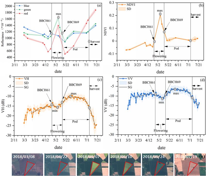
2860                                                                           J. Han et al.: The RapeseedMap10 database

2.2.4    Crop calendars                                          where green is the TOA reflectance of the green band (b3)
                                                                 of the S2 imagery, and blue is the blue band (b2) reflectance.
We used two crop phenological datasets to assist in the ex-      NDYI increased from −0.03 on 17 April to 0.21 on 7 May
traction of rapeseed phenological parameters: crop calendars     (Fig. 2b) and reached a peak during rapeseed flowering. This
in different countries (https://ipad.fas.usda.gov/ogamaps/       unique spectral feature of rapeseed during the flowering pe-
cropcalendar.aspx, last access: 8 June 2021) and field records   riod was due to the yellow petals.
of crop phenology in Germany. The crop calendars originated         S1 backscattering changes with rapeseed growth. We used
from the United States Department of Agriculture, which          VV and VH time series smoothed by the Savitzky–Golay
only records rapeseed planting and harvest times for selected    (SG) filter (window size 3) (Chen et al., 2004) as inputs to
countries. The crop phenology field records in Germany were      identify the phenological parameters of rapeseed parcels. We
in situ observations from crop phenological records shared       used the SG filter algorithm in MATLAB 2020b, which un-
by the Deutscher Wetterdienst (DWD) in Germany (Kas-             covered local minima in both the VV (−11.20, 8 May) and
par et al., 2014). The DWD provides field observations of        VH (−15.60, 5 May) time series during rapeseed flowering
crop phenological periods throughout Germany following           (Fig. 2c, d). Furthermore, VH reached a maximum (−9.64,
the Biologische Bundesanstalt, Bundessortenamt, and Chem-        1 June) during the pod period. Unlike other crops, rape-
ical Industry (BBCH) scale (Table 1). DWD records include        seed has two distinct green-up phases: the flowering period
the start and end dates of rapeseed flowering (d’Andrimont       and the pod period (Ashourloo et al., 2019; Bargiel, 2017;
et al., 2020; Kaspar et al., 2014). Neither the two crop cal-    Mercier et al., 2020; Veloso et al., 2017). The petals of rape-
endars nor the DWD records contain information on rape-          seed decrease the scattering of VV and VH, while the pods
seed peak flowering dates. To extract rapeseed phenological      increase the scattering intensity of VH (d’Andrimont et al.,
parameters, we used all stations that fully recorded start and   2020; Bargiel, 2017; McNairn et al., 2009; Mercier et al.,
end dates of the flowering period from 2017 to 2019, namely,     2020). The NDYI and backscattering (VV and VH) time se-
281, 269, and 253 stations in 2017, 2018, and 2019, respec-      ries of rapeseed in different climate regions (Fig. S1) exhib-
tively.                                                          ited the same characteristics. Therefore, we used both optical
                                                                 and SAR features to identify rapeseed flowering and pod pe-
2.3     Methods                                                  riods in this study. Because of differences in the revisit times
                                                                 of the S1/2 satellites, rapeseed peak flowering dates were de-
2.3.1    Optical and SAR characteristics during the              fined as the median dates extracted using optical and SAR
         rapeseed growing period                                 indicators.
We selected available rapeseed parcels and in situ observa-
tions of the DWD from different climate regions and differ-      2.3.2   Sample blocks collected for phenological
ent years to analyze the optical (reflectance and vegetation             monitoring
index) and SAR (VV and VH) characteristics of rapeseed
                                                                 As a prerequisite to large-scale mapping, the phenology of
over time. As an example, Fig. 2 shows the time series of one
                                                                 rapeseed in different countries must be identified and delin-
rapeseed parcel around a DWD station (station ID: 13126) in
                                                                 eated (Dong et al., 2016; Zhang et al., 2020), but not enough
2018. This rapeseed parcel exhibited unique visual charac-
                                                                 observational records of rapeseed phenology are available on
teristics during the flowering period (Fig. 2e). When rape-
                                                                 a large scale. In accordance with the DWD method of phe-
seed approached peak flowering, the flowers became yellow
                                                                 nological observation (Kaspar et al., 2014), we created sam-
(d’Andrimont et al., 2020; Pan et al., 2013; Tao et al., 2020;
                                                                 ple blocks with a radius of 10 km over rapeseed-producing
Wang et al., 2018). Rapeseed was yellow-green on the true-
                                                                 areas of different countries and randomly sampled 10 rape-
color images of S2 and Google Earth during the flowering
                                                                 seed parcels per block. The rapeseed plots were identified by
period (Fig. S1). The reflectance of the green and red bands
                                                                 their phenological characteristics, which were obtained by
separately increased – from 0.09 and 0.06, respectively, be-
                                                                 visual interpretation and analysis of reference data, including
fore flowering (17 April 2018) to 0.16 and 0.14 at peak flow-
                                                                 high-resolution images available in S2 and Google Earth as
ering (7 May 2018) – and then decreased (Fig. 2a). The re-
                                                                 well as spectral reflectance (red and green bands), spectral
flectance of the blue band was lower than that of the red and
                                                                 index (NDYI), and scattering coefficient profiles (VV and
green bands during flowering. This outcome is similar to the
                                                                 VH) from the S1/2 time series. Google Earth images taken
results of previous research (Ashourloo et al., 2019; Sulik
                                                                 during rapeseed flowering were used to assist with the visual
and Long, 2015). We also calculated the normalized differ-
                                                                 interpretation of rapeseed parcels. Rapeseed parcels with no
ence yellow index (NDYI), which can capture increasing yel-
                                                                 available high-quality time-series imagery were omitted. Fi-
lowness in a time series (d’Andrimont et al., 2020; Sulik and
                                                                 nally, 75 sample blocks in 2017, 84 sample blocks in 2018,
Long, 2016), as follows:
                                                                 and 84 sample blocks in 2019 were uniformly and randomly
          green − blue                                           collected (Fig. 1).
NDYI =                 ,                                   (1)
          green + blue

Earth Syst. Sci. Data, 13, 2857–2874, 2021                                       https://doi.org/10.5194/essd-13-2857-2021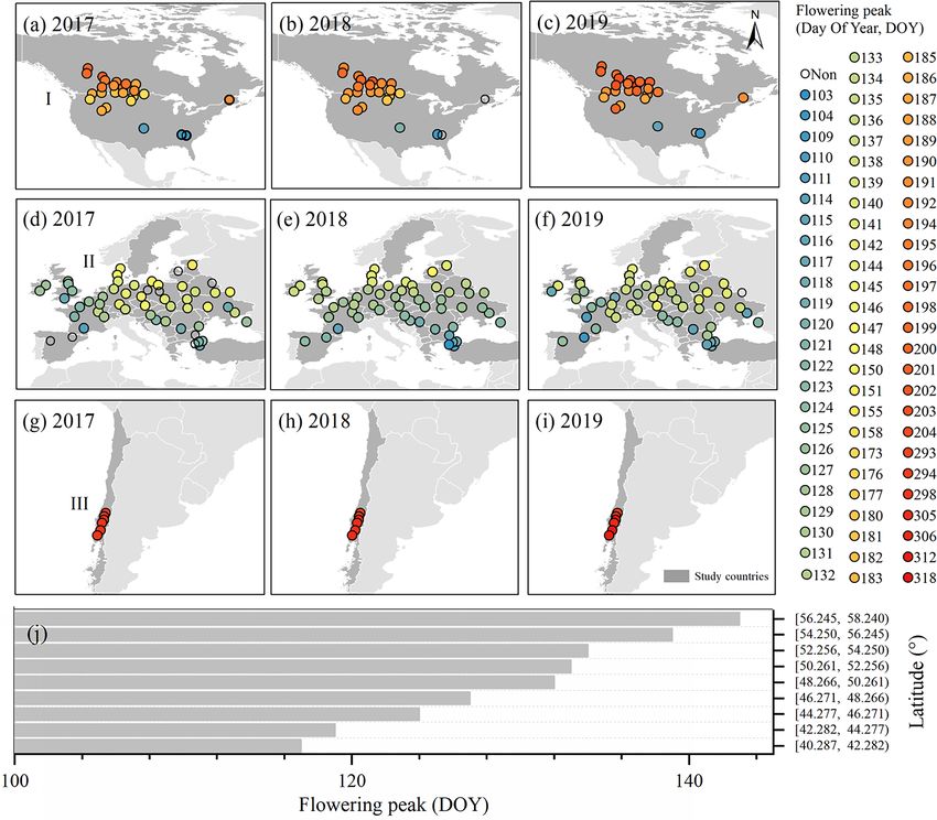
Table 1. Detailed information about the data collected in this work.

                                              Data                           Time          Resolution   Institution              Version    Data access                                   Last access    Descriptions
                                                                                                                                                                                          (yyyy/mm/dd)
                                              Sentinel-1 SAR GRD             2017–2019     10 m         European Space           –          https://developers.google.com/earth-engine/   2020/11/15     Extracting the backscatter coefficient
                                                                                                        Agency (ESA)                        datasets/catalog/COPERNICUS_S1_GRD                           characteristics of rapeseed
                                              Sentinel-2 MSI                 2017–2019     10 m         ESA                      Level-1C   https://developers.google.com/earth-engine/   2020/11/15     Calculating the spectral indices after re-
                                                                                                                                            datasets/catalog/COPERNICUS_S2                               moving the cloud

https://doi.org/10.5194/essd-13-2857-2021
                                              Global Food Security-Support   2015          30 m         United States Geologi-   V001       https://search.earthdata.nasa.gov/search?q=   2020/11/05     Identifying crop growing areas
                                                                                                                                                                                                                                                      J. Han et al.: The RapeseedMap10 database

                                              Analysis Data at 30 m                                     cal Survey,                         GFSAD30
                                              (GFSAD30)                                                 NASA et al.
                                              The Shuttle Radar Topography   –             30 m         NASA Jet Propulsion      V3         https://developers.google.com/earth-engine/   2020/10/01     Calculating slope map
                                              Mission (SRTM)                                            Laboratory                          datasets/catalog/USGS_SRTMGL1_003
                                              Cropland Data Layer (CDL)      2017, 2019    30 m         United States Depart-    –          https://developers.google.com/earth-engine/   2020/12/01     Accuracy verification of rapeseed map
                                                                                                        ment of Agriculture                 datasets/catalog/USDA_NASS_CDL                               at pixel level
                                              Annual Crop Inventory (ACI)    2017, 2018    30 m         Agriculture and          –          https://developers.google.com/earth-engine/   2020/12/01     Accuracy verification of rapeseed map
                                                                                                        Agri-Food Canada                    datasets/catalog/AAFC_ACI                                    at pixel level
                                              Crop Map of England            2018          hexagon      Rural Payments           V.09       https://data.gov.uk/dataset/                  2021/01/15     Accuracy verification of rapeseed map
                                              (CROME)                                      cells        Agency                              fb19d34f-59e6-48e7-820a-fe5fda3019e5/                        at pixel level
                                                                                                                                            crop-map-of-england-crome-2018
                                              Land Cover Map of France       2018          10 m         CNES/DNO/OT/PE           V1-0       https://www.theia-land.fr/en/                 2021/03/22     Accuracy verification of rapeseed map
                                              (LCMF)                                                                                        2018-land-cover-product/?cover-product/                      at pixel level
                                              Phenological database of       2017–2019     –            Deutsche Wetterdienst    –          https://www.dwd.de/DE/leistungen/cdc/         2020/10/01     Identifying the phenological character-
                                              Germany                                                   (DWD)                               climate-data-center.html?nn=575620&lsbId=                    istics of rapeseed
                                                                                                                                            646252
                                              Agricultural statistics data   2017–2019     –            Food and Agriculture     –          http://www.fao.org/faostat/en/#data/QC        2020/12/01     Verifying the accuracy of rapeseed map
                                                                                                        Organization (FAO)                                                                               at national scale
                                              Crop Calendars                 –             –            United States Depart-    –          https://ipad.fas.usda.gov/ogamaps/            2020/10/01     Auxiliary reference data for identifying
                                                                                                        ment of Agriculture                 cropcalendar.aspx                                            the flowering period of rapeseed

Earth Syst. Sci. Data, 13, 2857–2874, 2021
                                                                                                                                                                                                                                                      2861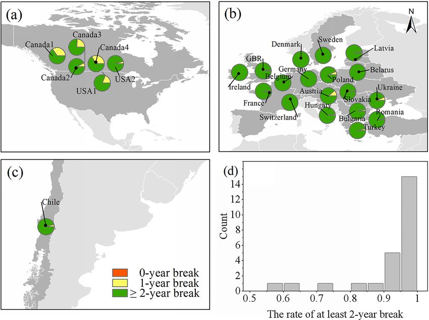
2862                                                                                 J. Han et al.: The RapeseedMap10 database

Figure 2. Time-series profiles of four features of rapeseed pixels around one DWD station (ID = 13126; longitude: 11.333268424◦ E,
latitude: 52.200000463◦ N) in Germany in 2018. (a) Mean reflectance values (red, green, and blue). (b) Mean NDYI. (c) Mean VH. (d)
Mean VV. The light-shaded areas indicate the standard deviation. The BBCH scale was used for in situ observations of rapeseed phenology,
with BBCH61 and BBCH69 respectively corresponding to the start and end of flowering. (e) The rapeseed parcel around the DWD station is
bounded in red (image source: Copernicus Sentinel-2 data 2018).

2.3.3   Detection of flowering and pod phases in different            Previous studies and field observation records have indicated
        countries                                                     that the flowering period of rapeseed is approximately 30 d
                                                                      (d’Andrimont et al., 2020; Chen et al., 2019; Kaspar et al.,
To determine the flowering dates of rapeseed in different             2014; She et al., 2015). Therefore, we divided each month
countries, we evaluated each phenological sample block                into two time periods, with the 15th day serving as the di-
from 2017 to 2019 (Fig. 3). First, we calculated the average          viding line. Two consecutive half-months were defined as a
values of all pixels in the 10 previously selected rapeseed           suitable period for classifying flowering dates (Fig. 4a–c).
parcels in each block during the rapeseed growth period in            Finally, we designated the flowering period for each admin-
conjunction with the crop calendar. VV and VH time series             istrative unit based on the sample blocks.
for each sampled rapeseed parcel were smoothed using the
SG filter. Second, S1/2 peak flowering dates and pod dates
were derived for all sample blocks according to the method            2.3.4   Development of a phenology- and pixel-based
in Sect. 2.3.1. We found that the peak flowering dates of rape-               algorithm for mapping rapeseed
seed, especially in Europe, followed an obvious latitudinal
gradient (Fig. 3j).                                                   Our temporal profiling of rapeseed parcels along with the re-
   We also observed that the signal with the maximum VH               sults of many previous studies indicated that the spectrum at
occurred within 45 d of the peak flowering date (Fig. S2). We         the flowering stage and the scattering signal at the pod stage
then calculated the difference in the peak flowering date of          are key features for identifying rapeseed (Ashourloo et al.,
each sample block between different years, which revealed             2019; Bargiel, 2017; Han et al., 2020; Mercier et al., 2020;
that the flowering peak dates of most sample parcels were             Sulik and Long, 2015; Veloso et al., 2017). We developed
advanced or delayed by only 10 d (Fig. 4d). Using the same            a single phenology- and pixel-based rapeseed mapping al-
period for different years in a given area was thus consid-           gorithm that relies on four features: spectral bands (red and
ered to be reasonable for rapeseed identification in this study.      green), spectral indices (NDYI), polarization bands (VH),

Earth Syst. Sci. Data, 13, 2857–2874, 2021                                             https://doi.org/10.5194/essd-13-2857-2021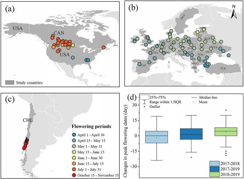
J. Han et al.: The RapeseedMap10 database                                                                                               2863

Figure 3. The spatial distribution of rapeseed flowering dates. (a)–(i) Flowering dates (Julian day) in different sample blocks in 2017, 2018,
and 2019. (j) Characteristics of the latitudinal gradient in Europe. The peak flowering date for each latitudinal interval is the mean of the
flowering dates of all sample blocks within that interval.

Figure 4. Flowering phenology of rapeseed. (a)–(c) The spatial distribution of rapeseed flowering periods among sample blocks. (d) Boxplot
showing changes in peak flowering dates of sample blocks over 3 years.

https://doi.org/10.5194/essd-13-2857-2021                                                 Earth Syst. Sci. Data, 13, 2857–2874, 2021
2864 J. Han et al.: The RapeseedMap10 database
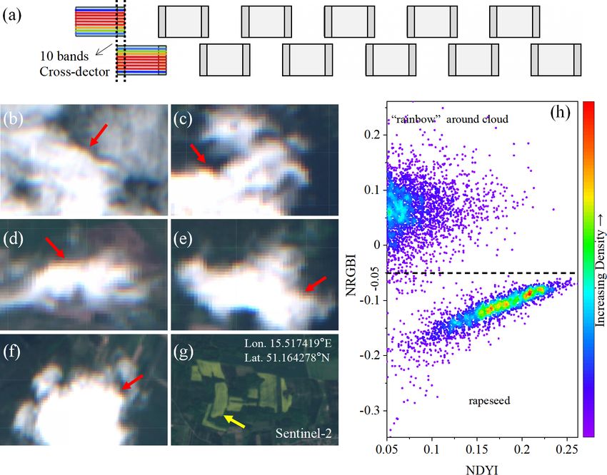
Figure 5. “Rainbow” cloud effect origins, examples, and solutions. (a) Staggered detector configuration of S2 (ESA, 2015a). (b)–(f) Exam-
ples of spectral misregistration effects and the performance of cloud-masking methods. Each image was masked with the quality assurance
band (QA60) for the Sentinel-2 TOA image. The red arrows indicate the “rainbow” appearing around clouds at high altitudes in the S2
image (image source: Copernicus Sentinel-2 data). (g) Sentinel-2 TOA image of rapeseed at the flowering stage. The yellow arrow indicates
rapeseed fields. (h) Scatter plot of NDYI vs. NRGBI of rapeseed field samples and samples with a “rainbow” around clouds in the S2 images.
Relative pixel density is indicated by the color scale on the right.
and terrain (slope). Four primary steps were used to map an- of the rainbow (Eq. 2):
nual planting areas (Fig. 6).
red − blue green − blue
In the first step, we determined the threshold of the fea- NRGBI = − , (2)
ture indicators. We analyzed the histograms of random sam- red + blue green + blue
ples selected from different countries as suggested by pre- where red, green, and blue are the TOA reflectance val-
vious study (Zou et al., 2018). Green and blue bands and ues of the red (b4), green (b3), and blue (b2) bands of
NDYI (Fig. S3) were similar during the flowering stage in the S2 imagery, respectively. A scatter plot of NDYI vs.
all samples from the different regions. Most rapeseed pix- NRGBI of rapeseed parcel samples and “rainbow” samples
els (98 %) had the following values: red > 0.07, green > 0.11, around clouds (visual interpretation) demonstrated that the
and NDYI > 0.05. We observed some pixels, however, with NRGBI (threshold = −0.05) can effectively distinguish rape-
a relatively high NDYI due to contamination by a cloud with seed from the rainbow (Fig. 5h). The GEE code for NRGBI
a “rainbow” appearance, which would cause them to be mis- index calculations can be found at https://code.earthengine.
classified as rapeseed (Fig. 5). Because of the limited qual- google.com/a39fc699a276d018778d59c5b085d960 (last ac-
ity of the QA band and the simple cloud score algorithm, cess: 8 June 2021). In addition, NRGBI can be calculated us-
such misclassifications arising from poor-quality observa- ing Eq. (2) in other GIS software programs (e.g., QGIS and
tions from the S2 image cannot be removed (X. Wang et al., ArcGIS) on a local computer.
2020b; Zhu et al., 2015). The rainbow in the cloud is the re- The second step was the identification of all rapeseed pix-
sult of the push-broom design of S2 (Fig. 5a) and spectral els from different images during the flowering period and
misregistration (for more details, see ESA, 2015a, and b). their subsequent aggregation into annual rapeseed planting
Taking into account the relative displacement of each spec- areas (Fig. 6). Because peak flowering dates and the number
tral channel sensor in the S2 push-broom design (Frantz et of available images of rapeseed fields vary within a region
al., 2018; X. Liu et al., 2020; Zhao et al., 2018), we devel- (Fig. S4), rapeseed classifications based on a single image
oped a new spectral index (NRGBI) to reduce the influence may fail to capture rapeseed flowering dynamics (Ashourloo
et al., 2019). To avoid misclassification due to poor-quality
Earth Syst. Sci. Data, 13, 2857–2874, 2021 https://doi.org/10.5194/essd-13-2857-2021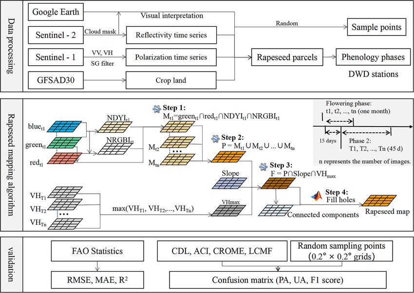
J. Han et al.: The RapeseedMap10 database                                                                                      2865

Figure 6. Workflow for mapping rapeseed areas using the proposed phenology- and pixel-based algorithm. GFSAD30, Global Food Security-
Support Analysis Data at 30 m; NDYI, normalized difference yellowness index; NRGBI, the new spectral index; DWD, Deutscher Wetter-
dienst; FAO, Food and Agriculture Organization of the United Nations; RMSE, root-mean-square error; MAE, mean absolute error; R 2 ,
R-squared; CDL, Cropland Data Layer; ACI, Annual Crop Inventory; CROME, Crop Map of England; LCMF, Land Cover Map of France;
UA, user’s accuracy; PA, producer’s accuracy; F1, F1 score.

observations during the rapeseed flowering stage, we aggre-           to remove objects not meeting a given threshold. The thresh-
gated all results classified from available S2 images during          olds of different indicators in different regions are given in
this period. The use of a larger number of images resulted in         Table S1.
better performance (Fig. S4).
   In the third step, we combined optical data with SAR im-           2.4   Accuracy assessment
ages to ensure the accuracy of the rapeseed maps. High VH
values during the pod stage are another distinct feature that         To test the accuracy of our proposed algorithm, we first com-
can distinguish rapeseed from other crops (Mercier et al.,            pared rapeseed areas retrieved using the new method with
2020; Tian et al., 2019; Van Tricht et al., 2018; Veloso et           FAO statistics. Our rapeseed data constituted a binary (0 or
al., 2017). Taking into consideration the variability of flow-        1) map with a spatial resolution of 10 m. We calculated the
ering in different fields and the duration of the pod stage           total area of rapeseed maps in each country and compared
(Sect. 2.3.2), we calculated the maximum VH between the               these numbers with FAO national rapeseed statistics. To ver-
second half of the flowering stage and the next 30 d (ca. 45 d;       ify the accuracy of rapeseed mapping, we used the RMSE
Fig. 6). Within this 45 d interval, at least three S1 satellite im-   (Eq. 3), MAE (Eq. 4), and coefficient of determination (R 2 ,
ages were available in the study area. In addition, areas with        Eq. 5), which were calculated as follows:
a slope ≥ 10◦ were removed (Jarasiunas, 2016). All pixels                        s
                                                                                   Xn (yi − fi )2
meeting these requirements were defined as rapeseed.                  RMSE =                            ,                        (3)
   In the fourth step, we removed “salt and pepper” noise by                             i=1       n
applying a threshold based on the number of connected com-                      1 Xn
                                                                      MAE =           i=1 i
                                                                                           |y − fi | ,                           (4)
ponents (objects), that is, the size of the neighborhood in pix-                n
els, and then filling the gaps inside the parcels (Hirayama et                   Pn                            2
                                                                                         (yi − yi )(fi − fi )
al., 2019). We used an eight-connected rule, which means              R 2 = P i=1                                  2 ,          (5)
                                                                                n               2 Pn
that the edges or corners of the pixels were connected. If                      i=1 (y i − y i )    i=1 f i − f  i
two adjacent pixels were connected, they were considered              where n is the total number of countries, yi is the mapped
part of the same object (https://www.mathworks.com/help/              rapeseed planting area for country i, yi is the corresponding
images/ref/bwareaopen.html, last access: 8 June 2021). The            mean value, fi is the rapeseed planting area recorded by the
bwareaopen function in MATLAB (version 2020b) was used                FAO for country i, and fi is the corresponding mean value.

https://doi.org/10.5194/essd-13-2857-2021                                            Earth Syst. Sci. Data, 13, 2857–2874, 2021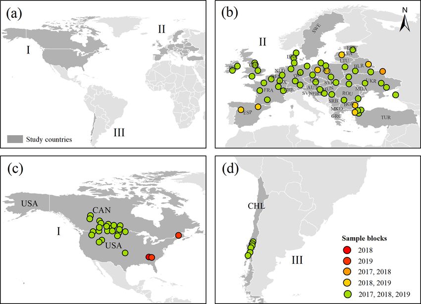
2866                                                                                 J. Han et al.: The RapeseedMap10 database

   We also compared our rapeseed maps with four open-
access datasets that include rapeseed layers at the pixel level:
ACI, CDL, CROME, and LCMF in Canada, the USA, GBR,
and France, respectively. We used the data from 2018 and
2019 in these datasets as a reference (Boryan et al., 2011;
Fisette et al., 2013). To unify the spatial resolution of our
rapeseed maps, we resampled CDL, ACI, and CROME to
10 m resolution to allow comparison. To check the accuracy
of our classification, we calculated UA (Eq. 6), PA (Eq. 7),
and F1 (Eq. 8) based on confusion matrices (Table S2).
   We also randomly selected verification samples based on
previous studies (Pekel et al., 2016; X. Wang et al., 2020a) to
validate our rapeseed maps. A 0.2◦ × 0.2◦ latitude–longitude
grid was superimposed on our 2018 rapeseed map (Fig. S5).
Two points – one rapeseed and the other non-rapeseed – were
randomly generated in each grid by visually interpreting im-
ages available from S2 and Google Earth along with spectral        Figure 7. Comparison of rapeseed areas with FAO statistics at the
reflectance (red and green bands), spectral index (NDYI), and      national level.
scattering coefficient (VV and VH) profiles from the S1/2
time series. Confusion matrices were similarly used to assess
accuracy according to Eqs. (6)–(8):
      xij
UA =       ,                                                (6)
       xj
      xij
PA =      ,                                                 (7)
      xi
           UA × PA
F1 = 2 ×           .                                        (8)
           UA + PA

In the above equations, xij is the value of the ith row and j th
column, xi is the sum of the ith row, and xj is the sum of the
j th column. Although the statistical data and existing prod-
ucts did not completely reflect the actual areas and locations
of cultivated rapeseed, these datasets were still beneficial for
validating the accuracy of our rapeseed maps at national and
pixel scales.
                                                                   Figure 8. Classification validation results. (a) Percentage of rape-
3     Results                                                      seed areas based on FAO statistics classified as such in existing
                                                                   products and our rapeseed map database. (b) Accuracy of our clas-
3.1    Accuracy assessment                                         sifications in four countries (Canada, USA, GBR, and France) us-
                                                                   ing existing products as a reference. UA, user’s accuracy; PA, pro-
We compared our derived rapeseed areas with those from             ducer’s accuracy; F1, F1 score.
FAO statistics. The total planting areas of rapeseed exhib-
ited good consistency with the agricultural statistics at the
national level, with a RMSE of 1459.64 km2 , a MAE of              (Table S3). As shown in Fig. 8a, the rapeseed areas calcu-
785.25 km2 , and an R 2 of 0.88 (Fig. 7). We found that the de-    lated from our maps were consistently more comparable to
rived areas in 2018 were larger than those in 2017 and 2019,       FAO statistics than those from existing products. UA, PA,
especially in countries with relatively small rapeseed areas.      and F1, which varied by country, ranged from 0.93–0.97,
The greater availability of S2 images and higher-quality data      0.70–0.80, and 0.81–0.86, respectively (Fig. 8b). The rape-
in 2018 may have contributed to the derivation of the larger       seed areas determined using our algorithm accounted for ap-
areas by our new method (X. Liu et al., 2020).                     proximately 71 % of the 2018 CDL, 71 % of the 2018 ACI,
   As indicated by their accuracy based on confusion matrix        80 % of the 2018 CROME, 70 % of the 2018 LCMF, and
values, our rapeseed maps were consistent at the pixel level       79 % of the 2019 CDL. In addition, the distributions on our
with maps of the American CDL in 2018 and 2019 and the             rapeseed maps were consistent with those of existing prod-
Canadian ACI, British CROME, and French LCMF in 2018               ucts at the pixel level (Figs. S7 and S8). The differences in

Earth Syst. Sci. Data, 13, 2857–2874, 2021                                             https://doi.org/10.5194/essd-13-2857-2021
J. Han et al.: The RapeseedMap10 database 2867
Figure 9. Spatially explicit details of rapeseed maps in eight countries with diverse crop structures in different years. The names of climate
zones are given in yellow. RGB composite images comprise red (b4), green (b3), and blue (b2) bands from Sentinel-2 good-quality obser-
vations during the rapeseed flowering period (image source: Copernicus Sentinel-2 data). Climate zone data are from the Food Insecurity,
Poverty and Environment Global GIS Database.
accuracy may have been due to the varied number of high- tions, ranging from a temperate oceanic climate (Fig. 9c–e)
quality images available in different regions (Dong et al., to temperate sub-continental (Fig. 9a, f) or even subtropical
2016). Despite the different ground conditions, methods, im- (Fig. 9b) ones, were clearly and comprehensively indicated
ages, and spatial resolutions among products, the results of on our maps. The fragmented pattern of land in some Euro-
our comparison further verify the accuracy of our rapeseed pean countries, especially that in eastern and central Europe
maps (Gong et al., 2020; Singha et al., 2019). due to land reform in 1989 (Hartvigsen, 2013, 2014), was
According to confusion matrix values (Table S4) based on clearly evident; Fig. 9f shows land in Estonia as an example
random sampling points, the accuracy of our rapeseed maps (Jürgenson and Rasva, 2020; Looga et al., 2018). Although
varied in different regions. We obtained the highest accuracy the algorithm was applied to different climates, terrains, and
(F1, 0.91) in zone II, followed by zone III (F1, 0.9), and zone landscapes over a very large region, its classification accu-
I (F1, 0.84). These disparities may be due to differences in racy across 33 countries was satisfactory. Our rapeseed maps
the availability of S1/2 images among the studied areas. can thus effectively identify fields in detail with high spatial
resolution and clear field boundaries. More rapeseed classifi-
3.2 Additional features of rapeseed maps derived using cation details can be found in Fig. S6.
our new method
3.3 Spatial patterns of rapeseed planting areas
To further characterize the rapeseed maps generated in this
study, we selected various images in several areas of each In our maps, the largest total area of rapeseed cultivation
country. The rapeseed maps showed good spatial consistency worldwide was in Canada. Along with GBR, Poland, and
with the actual areas of rapeseed cultivation on the ground Ukraine, the two leading rapeseed growing countries in Eu-
(Figs. 9 and S6). Fields with various planting densities, rang- rope – France and Germany – accounted for approximately
ing from densely planted areas in Canada (Fig. 9a) to rela- 66.3 % of European rapeseed areas. The 3-year (2017–2019)
tively sparse ones, such as in Chile (Fig. 9b) and European spatial patterns were consistent at the national level (Fig. S9).
countries (e.g., Fig. 9c, d) (Lowder et al., 2016); various We also plotted the geographic distribution of rapeseed ar-
shapes, ranging from regular rectangles (e.g., Fig. 9a, h) to eas along latitudinal and longitudinal gradients in the study
irregular parcels (Fig. 9c, d); and different climatic condi- areas (Fig. 10). With the exception of steep mountainous re-
https://doi.org/10.5194/essd-13-2857-2021 Earth Syst. Sci. Data, 13, 2857–2874, 20212868 J. Han et al.: The RapeseedMap10 database
Figure 10. Spatial distribution of rapeseed areas at 10 m resolution along latitudinal and longitudinal gradients in 2018. (a) Europe and
Turkey. (b) Canada and the USA.
gions and cold northern areas, rapeseed is widely planted in in crop yield management (Harker et al., 2015; X. Liu et al.,
European countries at latitudes of 46–53◦ N and longitudes 2018; Ren et al., 2015; Rudiyanto et al., 2019; Zhou et al.,
of 2◦ W–4◦ E, 9–19◦ E, and 22–27◦ E (Fig. 10a). In Canada 2015). To analyze rapeseed rotation patterns, we selected 25
and the USA, areas with latitudes of 49–54 and 56–57◦ N representative areas (Fig. S10) that met the following three
and longitudes of 117 to 118◦ W and 98 to 114◦ W have high criteria: high image quality, high rapeseed classification ac-
densities of planted rapeseed (Fig. 10b). curacy, and large extent of planted rapeseed. Rapeseed rota-
tion in these areas was calculated based on the frequency of
each rapeseed pixel (Fig. 11).
4 Discussion Because only 3 years (2017–2019) of rapeseed maps were
available, the longest observable rapeseed rotation break was
4.1 Investigation of rapeseed rotation systems 2 years. To more accurately discern the pattern of rapeseed
We obtained 3-year rapeseed maps at a spatial resolution of rotation, we thus classified rapeseed rotation breaks in this
10 m whose high accuracy was validated by annual national study into three types: ≥ 2 years, 1 year, and 0 years. Most
statistics books, open-access public products, and random countries, especially European ones, were characterized by
sampling points. These rapeseed maps provided a new op- rotation breaks that were ≥ 2 years (mostly green areas in
portunity to investigate rapeseed rotation systems (X. Liu et Fig. 12). In Canada, 70 % of fields were subjected to rota-
al., 2018). Crop rotation information is an important factor tion breaks of ≥ 2 years, with the remainder (30 %) follow-
Earth Syst. Sci. Data, 13, 2857–2874, 2021 https://doi.org/10.5194/essd-13-2857-2021J. Han et al.: The RapeseedMap10 database 2869
Figure 11. Spatial distribution of three rotation schedules in different areas from 2017–2019.
ing a 1-year break pattern (Fig. 12a). As shown in the his- 4.2 Uncertainty
togram in Fig. 12d, we identified 20 locations with ≥ 2-year
rotation breaks, which corresponds to 90 % of planting areas. The generation of annual high-resolution maps for a spe-
Many previous studies have found that a 2- or 3-year rotation cific crop over a large region is a major challenge (Dong et
break significantly reduces the number of fungal spores, es- al., 2016; Luo et al., 2020; Zhang et al., 2020). Pixel-and
pecially those of Rhizoctonia solani and Leptosphaeria mac- phenological-based algorithms, multisource remote sensing
ulans, thus suggesting that a rotation system is an important data, and the GEE are useful for mapping rapeseed at high
component of disease control in rapeseed (Gill, 2018; Harker resolution and over large areas. In addition to these advan-
et al., 2015; Ren et al., 2015; Zhou et al., 2015). Rapeseed tages, our proposed algorithm does not require large amounts
rotation also improves yield, moisture, and fertility and re- of training sample data and reduces disturbance due to agro-
duces weeds and pest insects (Bernard et al., 2012; Harker nomic differences by combining images from multiple dates.
et al., 2015; Pardo et al., 2015; Peng et al., 2015; Ren et al., Nevertheless, uncertainty still exists due to several issues.
2015). Additional efforts to produce longer time-series rape- The first of these factors is the cropland layer. We used
seed maps and acquire detailed rotation information are thus GFSAD30 datasets to identify cropland; however, the GF-
needed. SAD30 has limitations, such as classification errors (Phalke
et al., 2020). A second contributory aspect is the number
of satellite images available. Although our annual rapeseed
maps are consistent with FAO statistics and show higher ac-
curacy compared with existing products, they are limited by
https://doi.org/10.5194/essd-13-2857-2021 Earth Syst. Sci. Data, 13, 2857–2874, 20212870 J. Han et al.: The RapeseedMap10 database
Figure 12. Rapeseed crop rotation. (a)–(c) Proportions of rapeseed planting areas subjected to rotation breaks of 0, 1, or ≥ 2 years. (d) The
number of areas in (a)–(c) subjected to breaks of at least 2 years.
Figure 13. Example showing the effect of low-quality observations on classification accuracy. (a) Rapeseed map of an area of France
in 2017 that contains an error (longitude: 2.059824◦ E, latitude: 46.734987◦ N). (b) Availability of time-series Sentinel-2 images during
rapeseed flowering phases. (c) Comparison of the time series of different sites showing how the peak NDYI has been missed.
the quality of the observations during critical growth stages. ment can contribute to uncertainty. For example, landscape
For example, Fig. 13a shows an error in an area of France types might impact the accuracy of rapeseed maps (J. Wang
in 2017 that can be attributed to the lack of clear S2 images et al., 2020).
during the rapeseed flowering period (Fig. 13b). Because the
rapeseed flowering period is generally characterized by high
NDYI and high red and green band reflectance, rapeseed pix- 5 Data availability
els are likely to be misclassified if images are missing dur-
The rapeseed maps produced with 10 m resolution in this
ing the flowering stage (Fig. 13c). A third issue concerns the
study are accessible at Mendeley Data (http://dx.doi.org/10.
threshold for different indicators, which is a key factor for
17632/ydf3m7pd4j.3) (Han et al., 2021). The dataset in-
mapping crops (Ashourloo et al., 2019; Dong et al., 2016; X.
cludes a set of GeoTIFF images in the ESPG: 4326 spatial
Liu et al., 2020; J. Wang et al., 2020; Zhang et al., 2015).
reference system. The values 1 and 0 represent rapeseed and
Although reference thresholds for the three continents in this
non-rapeseed, respectively. We encourage users to indepen-
study are provided, they should be applied with caution to
dently verify the rapeseed maps. In addition, Sentinel 1/2 im-
other regions. Finally, the complexity of the ground environ-
ages, CDL, ACI, and SRTM are available on GEE (https://
Earth Syst. Sci. Data, 13, 2857–2874, 2021 https://doi.org/10.5194/essd-13-2857-2021J. Han et al.: The RapeseedMap10 database 2871
developers.google.com/earth-engine/datasets/, Google Earth References
Engine Data Catalog, 2021). For more detailed information
about the data collected in this work, see Table 1.
Arata, L., Fabrizi, E., and Sckokai, P.: A worldwide anal-
6 Conclusions ysis of trend in crop yields and yield variability: Ev-
idence from FAO data, Econ. Model., 90, 190–208,
Large-scale, high-resolution rapeseed maps are the basis for https://doi.org/10.1016/j.econmod.2020.05.006, 2020.
crop growth monitoring and yield prediction. We developed a Ashourloo, D., Shahrabi, H. S., Azadbakht, M., Aghighi,
new method for mapping rapeseed based on spectral and po- H., Nematollahi, H., Alimohammadi, A., and Matkan,
larization features and multi-source data. We used the new al- A. A.: Automatic canola mapping using time series of
sentinel 2 images, ISPRS J. Photogramm., 156, 63–76,
gorithm to produce three annual rapeseed maps (2017–2019)
https://doi.org/10.1016/j.isprsjprs.2019.08.007, 2019.
at 10 m spatial resolution in 33 countries. According to the Bargiel, D.: A new method for crop classification com-
results of three different verification methods, our rapeseed bining time series of radar images and crop phenol-
maps are reasonably accurate. Compared with existing prod- ogy information, Remote Sens. Environ., 198, 369–383,
ucts at the pixel level in Canada, USA, GBR, and France, PA, https://doi.org/10.1016/j.rse.2017.06.022, 2017.
UA, and F1 were 0.70–0.80, 0.93–0.97, and 0.81–0.86, re- Bartholomé, E. and Belward, A. S.: GLC2000: a new ap-
spectively. In addition, F1 ranged from 0.84 to 0.91 based on proach to global land cover mapping from Earth ob-
independent validation samples. Our approach reduces mis- servation data, Int. J. Remote Sens., 26, 1959–1977,
classifications due to different planting times and low-quality https://doi.org/10.1080/01431160412331291297, 2005.
observations to some degree. The 10 m rapeseed maps pro- Bernard, E., Larkin, R. P., Tavantzis, S., Erich, M. S., Alyokhin,
vide more spatial details of rapeseed. Finally, we observed A., Sewell, G., Lannan, A., and Gross, S. D.: Compost,
rapeseed rotation, and biocontrol agents significantly im-
that the rapeseed crop rotation interval is at least 2 years
pact soil microbial communities in organic and conven-
in almost all countries in this study. Our proposed rapeseed tional potato production systems, Appl. Soil Ecol., 52, 29–41,
mapping method can be applied to other regions. The derived https://doi.org/10.1016/j.apsoil.2011.10.002, 2012.
rapeseed data product is useful for many purposes, including Boryan, C., Yang, Z., Mueller, R., and Craig, M.: Mon-
crop growth monitoring and production and rotation system itoring US agriculture: the US Department of Agri-
planning. culture, National Agricultural Statistics Service, Crop-
land Data Layer Program, Geocarto Int., 26, 341–358,
https://doi.org/10.1080/10106049.2011.562309, 2011.
Supplement. The supplement related to this article is available Carré, P. and Pouzet, A.: Rapeseed market, worldwide and in
online at: https://doi.org/10.5194/essd-13-2857-2021-supplement. Europe, OCL, 21, D102, https://doi.org/10.1051/ocl/2013054,
2014.
Chen, B., Jin, Y., and Brown, P.: An enhanced bloom in-
Author contributions. ZZ and JH designed the research. JH and dex for quantifying floral phenology using multi-scale remote
YL collected datasets. JH implemented the research and wrote the sensing observations, ISPRS J. Photogramm., 156, 108–120,
paper. ZZ, JC, LZ, JZ, and ZL revised the paper. https://doi.org/10.1016/j.isprsjprs.2019.08.006, 2019.
Chen, J., Jönsson, P., Tamura, M., Gu, Z., Matsushita, B.,
and Eklundh, L.: A simple method for reconstructing
a high-quality NDVI time-series data set based on the
Competing interests. The authors declare that they have no
Savitzky–Golay filter, Remote Sens. Environ., 91, 332–344,
known competing financial interests or personal relationships that
https://doi.org/10.1016/j.rse.2004.03.014, 2004.
could have appeared to influence the work reported in this paper.
d’Andrimont, R., Taymans, M., Lemoine, G., Ceglar, A.,
Yordanov, M., and van der Velde, M.: Detecting flower-
ing phenology in oil seed rape parcels with Sentinel-1
Acknowledgements. We thank the editor and the two anony- and -2 time series, Remote Sens. Environ., 239, 111660,
mous referees for their valuable comments. We thank Liwen Bianji https://doi.org/10.1016/j.rse.2020.111660, 2020.
(Edanz) (https://www.liwenbianji.cn, last access: 8 June 2021) for Dong, J., Xiao, X., Menarguez, M. A., Zhang, G., Qin, Y., Thau, D.,
editing the language of a draft of this paper. Biradar, C., and Moore, B.: Mapping paddy rice planting area in
northeastern Asia with Landsat 8 images, phenology-based al-
gorithm and Google Earth Engine, Remote Sens. Environ., 185,
Financial support. This research has been supported by the Na- 142–154, https://doi.org/10.1016/j.rse.2016.02.016, 2016.
tional Key Research and Development Program of China (grant no. Drusch, M., Del Bello, U., Carlier, S., Colin, O., Fernandez,
2019YFA0607401). V., Gascon, F., Hoersch, B., Isola, C., Laberinti, P., Marti-
mort, P., Meygret, A., Spoto, F., Sy, O., Marchese, F., and
Bargellini, P.: Sentinel-2: ESA’s Optical High-Resolution Mis-
Review statement. This paper was edited by David Carlson and sion for GMES Operational Services, Remote Sens. Environ.,
reviewed by two anonymous referees. 120, 25–36, https://doi.org/10.1016/j.rse.2011.11.026, 2012.
https://doi.org/10.5194/essd-13-2857-2021 Earth Syst. Sci. Data, 13, 2857–2874, 20212872 J. Han et al.: The RapeseedMap10 database
ESA: Sentinel-2 products specification document, available Google Earth Engine Data Catalog: A planetary-scale platform for
at: https://sentinel.esa.int/documents/247904/349490/S2_MSI_ Earth science data & analysis, available at: https://developers.
Product_Specification.pdf (last access: 24 April 2019), 2015a. google.com/earth-engine/datasets/, last access: 8 June 2021
ESA: Data Product Quality Reports, available at: Gorelick, N., Hancher, M., Dixon, M., Ilyushchenko, S., Thau, D.,
https://sentinels.copernicus.eu/documents/247904/ and Moore, R.: Google Earth Engine: Planetary-scale geospatial
3902831/Sentinel-2_L1C_Data_Quality_Report/ analysis for everyone, Remote Sensing of Environment, 202, 18–
adfff903-a337-4fc1-9439-558456bad0b1?version=1.1 (last 27, https://doi.org/10.1016/j.rse.2017.06.031, 2017.
access: 8 June 2021), 2015b. Griffiths, P., Nendel, C., and Hostert, P.: Intra-annual reflectance
Fang, S., Tang, W., Peng, Y., Gong, Y., Dai, C., Chai, R., and Liu, composites from Sentinel-2 and Landsat for national-scale crop
K.: Remote Estimation of Vegetation Fraction and Flower Frac- and land cover mapping, Remote Sens. Environ., 220, 135–151,
tion in Oilseed Rape with Unmanned Aerial Vehicle Data, Re- https://doi.org/10.1016/j.rse.2018.10.031, 2019.
mote Sensing, 8, 416, https://doi.org/10.3390/rs8050416, 2016. Han, J., Zhang, Z., and Cao, J.: Developing a New Method
Farr, T. G., Rosen, P. A., Caro, E., Crippen, R., Duren, R., to Identify Flowering Dynamics of Rapeseed Using
Hensley, S., Kobrick, M., Paller, M., Rodriguez, E., Roth, Landsat 8 and Sentinel-1/2, Remote Sensing, 13, 105,
L., Seal, D., Shaffer, S., Shimada, J., Umland, J., Werner, https://doi.org/10.3390/rs13010105, 2020.
M., Oskin, M., Burbank, D., and Alsdorf, D.: The Shut- Han, J., Zhang, Z., Luo, Y., Cao, J., Zhang, L., Zhang,
tle Radar Topography Mission, Rev. Geophys., 45, RG2004, J., and Li, Z.: Data for: Developing a phenology- and
https://doi.org/10.1029/2005RG000183, 2007. pixel-based algorithm for mapping rapeseed at 10m spa-
Firrisa, M. T., van Duren, I., and Voinov, A.: Energy efficiency for tial resolution using multi-source data, Mendeley Data, V3,
rapeseed biodiesel production in different farming systems, En- https://doi.org/10.17632/ydf3m7pd4j.3, 2021.
erg. Effic., 7, 79–95, https://doi.org/10.1007/s12053-013-9201-2, Harker, K. N., O’Donovan, J. T., Turkington, T. K., Blackshaw,
2014. R. E., Lupwayi, N. Z., Smith, E. G., Johnson, E. N., Gan, Y.,
Fisette, T., Rollin, P., Aly, Z., Campbell, L., Daneshfar, B., Filyer, Kutcher, H. R., Dosdall, L. M., and Peng, G.: Canola rotation
P., Smith, A., Davidson, A., Shang, J., and Jarvis, I.: AAFC frequency impacts canola yield and associated pest species, Can.
annual crop inventory, in: 2013 Second International Con- J. Plant Sci., 95, 9–20, https://doi.org/10.4141/cjps-2014-289,
ference on Agro-Geoinformatics (Agro-Geoinformatics), 2015.
IEEE, Fairfax, VA, USA, https://doi.org/10.1109/Argo- Hartvigsen, M.: Land reform in Central and Eastern Europe after
Geoinformatics.2013.6621920, pp. 270–274, 2013. 1989 and its outcome in the form of farm structures and land
Frantz, D., Haß, E., Uhl, A., Stoffels, J., and Hill, J.: Improvement fragmentation, FAO Land Tenure Working Paper 24, Food and
of the Fmask algorithm for Sentinel-2 images: Separating clouds Agriculture Organization of the United Nations, Rome, Italy,
from bright surfaces based on parallax effects, Remote Sens. En- 2013.
viron., 215, 471–481, https://doi.org/10.1016/j.rse.2018.04.046, Hartvigsen, M.: Land reform and land fragmentation in Cen-
2018. tral and Eastern Europe, Land Use Policy, 36, 330–341,
Fuglie, K. O.: Total factor productivity in the global agricultural https://doi.org/10.1016/j.landusepol.2013.08.016, 2014.
economy: Evidence from FAO data, in: The shifting patterns of Hassan, M. Hj. and Kalam, Md. A.: An Overview of
agricultural production and productivity worldwide, edited by: Biofuel as a Renewable Energy Source: Develop-
Alston, J. M., Babcock, B., and Pardey, P. G., Midwest Agribusi- ment and Challenges, Procedia Engineer., 56, 39–53,
ness Trade and Research Information Center, Ames, Iowa, 63– https://doi.org/10.1016/j.proeng.2013.03.087, 2013.
95, 2010. Hirayama, H., Sharma, R. C., Tomita, M., and Hara, K.: Eval-
Gill, K. S.: Crop rotations compared with continuous canola uating multiple classifier system for the reduction of salt-
and wheat for crop production and fertilizer use over 6 yr, and-pepper noise in the classification of very-high-resolution
edited by: Willenborg, C., Can. J. Plant Sci., 98, 1139–1149, satellite images, Int. J. Remote Sens., 40, 2542–2557,
https://doi.org/10.1139/cjps-2017-0292, 2018. https://doi.org/10.1080/01431161.2018.1528400, 2019.
Gong, P., Wang, J., Yu, L., Zhao, Y., Zhao, Y., Liang, L., Niu, Z., Höök, M. and Tang, X.: Depletion of fossil fuels and anthro-
Huang, X., Fu, H., Liu, S., Li, C., Li, X., Fu, W., Liu, C., Xu, pogenic climate change – A review, Energ. Policy, 52, 797–809,
Y., Wang, X., Cheng, Q., Hu, L., Yao, W., Zhang, H., Zhu, P., https://doi.org/10.1016/j.enpol.2012.10.046, 2013.
Zhao, Z., Zhang, H., Zheng, Y., Ji, L., Zhang, Y., Chen, H., Yan, Inglada, J., Vincent, A., Arias, M., Tardy, B., Morin, D., and Rodes,
A., Guo, J., Yu, L., Wang, L., Liu, X., Shi, T., Zhu, M., Chen, I.: Operational High Resolution Land Cover Map Production at
Y., Yang, G., Tang, P., Xu, B., Giri, C., Clinton, N., Zhu, Z., the Country Scale Using Satellite Image Time Series, Remote
Chen, J., and Chen, J.: Finer resolution observation and mon- Sensing, 9, 95, https://doi.org/10.3390/rs9010095, 2017.
itoring of global land cover: first mapping results with Land- Jarasiunas, G.: Assessment of the agricultural land under steep
sat TM and ETM+ data, Int. J. Remote Sens., 34, 2607–2654, slope in Lithuania, J. Cent. Eur. Agric., 17, 176–187,
https://doi.org/10.1080/01431161.2012.748992, 2013. https://doi.org/10.5513/JCEA01/17.1.1688, 2016.
Gong, P., Li, X., Wang, J., Bai, Y., Chen, B., Hu, T., Jürgenson, E. and Rasva, M.: The Changing Structure and
Liu, X., Xu, B., Yang, J., Zhang, W., and Zhou, Y.: An- Concentration of Agricultural Land Holdings in Esto-
nual maps of global artificial impervious area (GAIA) be- nia and Possible Threat for Rural Areas, Land, 9, 41,
tween 1985 and 2018, Remote Sens. Environ., 236, 111510, https://doi.org/10.3390/land9020041, 2020.
https://doi.org/10.1016/j.rse.2019.111510, 2020. Kaspar, F., Zimmermann, K., and Polte-Rudolf, C.: An overview
of the phenological observation network and the pheno-
Earth Syst. Sci. Data, 13, 2857–2874, 2021 https://doi.org/10.5194/essd-13-2857-2021You can also read