The sensitivity of the Greenland Ice Sheet to glacial-interglacial oceanic forcing - Climate of the Past
←
→
Page content transcription
If your browser does not render page correctly, please read the page content below
Clim. Past, 14, 455–472, 2018
https://doi.org/10.5194/cp-14-455-2018
© Author(s) 2018. This work is distributed under
the Creative Commons Attribution 4.0 License.

The sensitivity of the Greenland Ice Sheet to
glacial–interglacial oceanic forcing
Ilaria Tabone1,2 , Javier Blasco1,2 , Alexander Robinson1,2,a , Jorge Alvarez-Solas1,2 , and Marisa Montoya1,2
1 Universidad Complutense de Madrid, 28040 Madrid, Spain
2 Institutode Geociencias, Consejo Superior de Investigaciones Cientificas-Universidad Complutense de Madrid,
28040 Madrid, Spain
a now at: Faculty of Geology and Geoenvironment, University of Athens, 15784 Athens, Greece

Correspondence: Ilaria Tabone (itabone@ucm.es)

Received: 2 October 2017 – Discussion started: 8 November 2017
Revised: 9 March 2018 – Accepted: 13 March 2018 – Published: 9 April 2018

Abstract. Observations suggest that during the last decades       1   Introduction
the Greenland Ice Sheet (GrIS) has experienced a gradually
accelerating mass loss, in part due to the observed speed-        Recent observations show that the Greenland Ice Sheet
up of several of Greenland’s marine-terminating glaciers.         (GrIS) has lost mass at an accelerated rate over the
Recent studies directly attribute this to warming North At-       past decades (Rignot et al., 2011; Zwally et al., 2011;
lantic temperatures, which have triggered melting of the out-     Sasgen et al., 2012; Shepherd et al., 2012; van den
let glaciers of the GrIS, grounding-line retreat and enhanced     Broeke et al., 2016). On average, the GrIS contributed to
ice discharge into the ocean, contributing to an acceleration     0.47 ± 0.23 mm a−1 of sea-level rise from 1991 to 2015
of sea-level rise. Reconstructions suggest that the influence     (van den Broeke et al., 2016), with an accelerated rate of
of the ocean has been of primary importance in the past as        0.89 ± 0.09 mm a−1 from 2010 to 2014 (Yi et al., 2015). In
well. This was the case not only in interglacial periods, when    the future, the GrIS is expected to continue losing mass,
warmer climates led to a rapid retreat of the GrIS to land        contributing to a sea-level rise relative to the 20th cen-
above sea level, but also in glacial periods, when the GrIS       tury between 90 and 280 mm by 2100 in the worst-case
expanded as far as the continental shelf break and was thus       scenario (RCP8.5) (Bindschadler et al., 2013; IPCC, 2013;
more directly exposed to oceanic changes. However, the GrIS       Clark et al., 2015; Fürst et al., 2015). This accelerated ice
response to palaeo-oceanic variations has yet to be investi-      loss is due to a combination of increased surface melting
gated in detail from a mechanistic modelling perspective. In      and enhanced ice discharge from marine-terminating glaciers
this work, the evolution of the GrIS over the past two glacial    to the ocean (van den Broeke et al., 2016). High surface
cycles is studied using a three-dimensional hybrid ice-sheet–     melting has been attributed to rising atmospheric Greenland
shelf model. We assess the effect of the variation of oceanic     temperatures (Box et al., 2009; Hall et al., 2008; Tedesco
temperatures on the GrIS evolution on glacial–interglacial        et al., 2016), which may also increase crevassing and calv-
timescales through changes in submarine melting. The re-          ing at the ice front. Conversely, the recently enhanced dis-
sults show a very high sensitivity of the GrIS to changing        charge of ice into the ocean is thought to be directly con-
oceanic conditions. Oceanic forcing is found to be a primary      nected to warmer Atlantic waters entering Greenland’s fjords
driver of GrIS expansion in glacial times and of retreat in in-   (Holland et al., 2008a; Rignot et al., 2010; Straneo et al.,
terglacial periods. If switched off, palaeo-atmospheric vari-     2010; Straneo and Heimbach, 2013). Higher oceanic tem-
ations alone are not able to yield a reliable glacial configu-    peratures increase the submarine melting at the calving front
ration of the GrIS. This work therefore suggests that consid-     of tidewater glaciers, contributing to their acceleration, ice
ering the ocean as an active forcing should become standard       mass discharge into the ocean and potentially grounding-line
practice in palaeo-ice-sheet modelling.                           retreat. This acceleration-and-retreat mechanism has been
                                                                  found in several Greenland glaciers that terminate in the

Published by Copernicus Publications on behalf of the European Geosciences Union.
456                                                                 I. Tabone et al.: The sensitivity of the Greenland Ice Sheet

ocean (Rignot and Kanagaratnam, 2006). Jakobshavn Isbræ,            water depth below the ice shelves. Under this assumption,
West Greenland’s fastest glacier, experienced a high rate of        the submarine melt rate increases when the past sea-level
basal melting (Motyka et al., 2011) initially induced by the        rises. However, their approach does not take into account
intrusion of warmer waters from the Irminger Sea (Holland           ocean temperature changes. Other studies have reconstructed
et al., 2008a), more than doubling its speed in the last 25         the GrIS past evolution as driven essentially by atmospheric
years (Joughin et al., 2012) and suffering a rapid retreat of its   forcing (Langebroek and Nisancioglu, 2016; Quiquet et al.,
terminus. Following enhanced subglacial melting observed            2012, 2013; Robinson et al., 2011; Stone et al., 2013), while
in the early 2000s, the Helheim Glacier (southeast Green-           the dynamic evolution of the entire GrIS including the influ-
land) also doubled its speed (Howat et al., 2005; Suther-           ence of the past oceanic forcing too has only been investi-
land and Straneo, 2012) and suffered peak thinning rates of         gated in a simplified manner. To this end, Huybrechts (2002)
90 m a−1 (Stearns and Hamilton, 2007), with its terminus re-        used a three-dimensional ice-sheet model in which marine
treating by about 7 km over just 3 years (Howat et al., 2007;       extent is controlled by changes in water depth based on
Straneo et al., 2016).                                              past eustatic sea-level variations, while Tarasov and Peltier
   The complex mechanisms that lead to ice-shelf thinning,          (2002), Simpson et al. (2009) and Lecavalier et al. (2014)
loss of buttressing and potential grounding-line instability        performed a palaeo-reconstruction of the entire GrIS con-
have been studied largely for the Antarctic Ice Sheet (AIS)         straining their ice-sheet models with past relative sea-level
(DeConto and Pollard, 2016; Favier et al., 2014; Hanna et al.,      (RSL) reconstructions. However, submarine melting was not
2013; Joughin et al., 2014a; Pritchard et al., 2012; Rignot         taken into account as an active forcing in these studies.
et al., 2004; Shepherd et al., 2004; Wouters et al., 2015).            The main purpose of this work is to assess the impact
The thinning of the Larsen C ice shelf (Holland et al., 2015)       of ice–ocean interaction on the evolution of the whole GrIS
and its recent calving event (Hogg and Gudmundsson, 2017;           throughout the last two glacial cycles. By implementing a
Jansen et al., 2015), the collapse of Larsen B and the melt-        submarine melting rate parameterization suitable for palaeo-
ing of the Antarctic Peninsula glaciers (Cook et al., 2016),        climatic studies into a three-dimensional hybrid ice-sheet–
the widespread retreat of Pine Island and other glaciers in         shelf model, we evaluate the sensitivity of the GrIS to
West Antarctica (Alley et al., 2015; Joughin et al., 2014b;         past climatic variations, including changes in oceanic tem-
Rignot et al., 2014) and the thinning of some East Antarc-          peratures (in terms of heat-flux variations), and investigate
tica ice shelves (Rignot et al., 2013) are notable examples         their capability to trigger grounding-line advance and retreat
of the direct connection between changes in oceanic forcing         through time. First, we describe the ice-sheet–shelf model
and glacier-termini adjustment (Alley et al., 2015). Only in        used to simulate the GrIS evolution, focusing on the imple-
the last several years has the scientific community also fo-        mentation of the submarine melt rate parameterization, and
cused its attention on the ice–ocean interaction in Greenland,      the sensitivity tests performed for this study (Sect. 2). In
motivated by the observed acceleration and retreat of major         Sect. 3, we show the results obtained in each experiment and
GrIS outlet glaciers. Although marine-terminating glaciers          we compare them with data for the last interglacial (LIG),
cover only a small fraction of the entire GrIS, modifications       the Last Glacial Maximum (LGM) and the present day (PD)
at the ice–ocean boundaries due to oceanic changes may              found in the literature. After discussing the main model un-
considerably affect the inland ice geometry. The effects in-        certainties and caveats (Sect. 4), we summarize the main con-
duced by outlet-glacier acceleration are transferred onshore        clusions of this work (Sect. 5).
by ice-flow dynamics, causing adjustments to the entire in-
land ice-mass configuration (Nick et al., 2009; Fürst et al.,
                                                                    2     Model description and experimental design
2013; Golledge et al., 2012). For this reason, a full under-
standing of the interaction between ice and ocean is crucial        2.1    Model
to assess the response of the GrIS to past and future climate
changes.                                                            To investigate the oceanic sensitivity of the GrIS throughout
   Various numerical models have been used to simulate cur-         the last two glacial cycles, we use the three-dimensional, hy-
rent submarine melt rates (Jenkins, 2011; Rignot et al., 2016;      brid, ice-sheet–shelf model GRISLI-UCM. The model is an
Sciascia et al., 2013; Xu et al., 2012, 2013) and dynamic re-       extension of the GRISLI ice-sheet model (Ritz et al., 2001),
treat (Morlighem et al., 2016; Vieli and Nick, 2011) of the         which has already been successfully used to simulate the
GrIS marine-terminating glaciers, as well as ice-dynamic fu-        evolution of the past Greenland (Quiquet et al., 2012, 2013)
ture projections of the whole GrIS (Fürst et al., 2015; Now-        and Antarctic ice sheets (Ritz et al., 2001; Philippon et al.,
icki et al., 2013), due to changes in the oceanic temperatures.     2006; Alvarez-Solas et al., 2010), as well as the Laurentide
However, how this thermal forcing affected the past GrIS            Ice Sheet (Alvarez-Solas et al., 2011, 2013). GRISLI-UCM
configuration has not been explored from a modelling per-           combines the Shallow Ice Approximation (SIA) for slow in-
spective so far. Recently, Bradley et al. (2017) simulated the      land deformational flow and the Shallow Shelf Approxima-
GrIS evolution for the two last glacial cycles by considering       tion (SSA) over fast-flowing areas, that is, ice streams and ice
a sub-shelf melt parameterization which is a function of the        shelves, where plug flow is dominant. Since we assume de-

Clim. Past, 14, 455–472, 2018                                                                   www.clim-past.net/14/455/2018/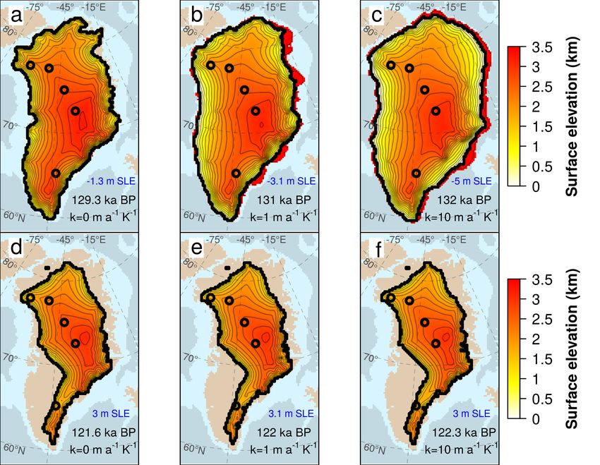
I. Tabone et al.: The sensitivity of the Greenland Ice Sheet                                                                      457

formational ice-sheet regions to be frozen at the bedrock, no       as it omits the contribution of insolation-induced effects on
basal sliding is considered for SIA-dominated areas. Basal          surface melting, which are important in past warmer periods
sliding for ice streams is determined through a basal drag          such as the Eemian (Robinson and Goelzer, 2014). However,
term (τ b ), defined as a function of the effective pressure        since this study focuses on the melting effects induced by
(Neff ) between ice and water pressure, and the basal hori-         past ocean temperature variations, the PDD melt model is
zontal velocity (ub ), considered as follows:                       sufficient to give a first approximation of surface melt that
                                                                    allows the ice sheet to retreat during interglacial periods in
τ b = −β ub ,                                                (1)    a realistic way. The atmospheric temperature forcing is a
                                                                    spatially and temporally variable field. It is retrieved using
where
                                                                    an index-anomaly approach in which the present-day clima-
β ∝ Neff .                                                   (2)    tological field (Tclim, atm ) is perturbed by past temperature
                                                                    anomalies derived through a spatially uniform climatic index
Dragging at the floating ice-shelf base is considered to be         α(t) (Fig. 1), as follows:
zero. The position of the grounding line is evaluated follow-
ing a flotation rule dependent on the current sea level and         Tatm (t) = Tclim, atm + (1 − α(t)) (TLGM, atm − TPD, atm ).   (5)
the ice thickness. Calving at the ice front is based on a two-
condition thickness criterion (Peyaud et al., 2007; Colleoni        The index α(t) is built through a multiproxy approach. First,
et al., 2014). First, an ice-shelf front must have a thickness      we combine the temperature reconstruction for Greenland by
lower than 200 m to potentially contribute to ice discharge.        Vinther et al. (2009) from 11.7 ka BP to present, the North
This threshold is in agreement with the thickness of many           Greenland Ice Core Project (NGRIP) reconstruction (Kindler
observed shelves at their ice–ocean interface. Second, if the       et al., 2014) for 115–11.7 ka BP and the North Greenland
ice advected from each upstream point is not sufficient to          Eemian Ice Drilling (NEEM) reconstruction (NEEM, 2013)
maintain the ice-front thickness higher than that threshold,        for 135–115 ka BP, and we generate a synthetic temperature
the grid point at the front calves. The entire GrIS ice dy-         anomaly time series for 250–135 ka BP based on Antarctic
namics is solved on a computational grid of 20 km × 20 km           isotope records following Barker et al. (2011). Second, the
horizontal resolution and 21 vertical layers. The glacial iso-      composite signal undergoes a windowed low-pass frequency
static adjustment (GIA) is described by the elastic lithosphere     filter (fc = 1/16 ka−1 ) in order to remove the spectral com-
– relaxed asthenosphere method (Le Meur and Huybrechts,             ponents associated with millennial timescales and below. Fi-
1996), for which the viscous asthenosphere responds to the          nally, the index α is obtained by normalizing the resulting
ice load with a tunable characteristic relaxation time (see         signal to be in agreement with Eq. (5), i.e. α = 0 for the LGM
Sect. 2.4).                                                         and α = 1 for the present day. The present-day climatological
   The hybrid scheme uses a weighting function to combine           field is taken from the regional climate model MAR forced
the non-sliding horizontal SIA velocities (uSIA ) with the SSA      by ERA-Interim (Fettweis et al., 2013). TLGM, atm − TPD, atm
horizontal velocities (uSSA ) and is defined as (Bueler and         is the 2-D surface atmospheric temperature (SAT) differ-
Brown, 2009)                                                        ence between the LGM and the present, as simulated by
                                                                    the climatic model of intermediate complexity CLIMBER-
u = (1 − f (uSSA )) uSIA + f (uSSA ) uSSA ,                  (3)    3α (Montoya and Levermann, 2008). For the precipitation
                                                                    rate, the procedure is similar, but the annual present-day pre-
where the weighting function f (uSSA ) depends on the mod-          cipitation is scaled by the ratio of the past precipitation to its
ule of the SSA component (uSSA ) through                            present value, as in Banderas et al. (2017). At the base of the
                                                                    grounded ice, the melt rate is calculated as a function of the
                         uSSA 2

              2
f (uSSA ) =     arctan          ,                            (4)    geothermal heat flux, which is prescribed following Shapiro
              π          uref                                       and Ritzwoller (2004), and the local pressure melting point.
ranging between 0 and 1. In this work, the reference velocity       The submarine melt rate is described in detail in the next sub-
uref is set to 100 m a−1 . For small values of uSSA , f (uSSA ) ≈   section.
0 and the horizontal velocities are calculated within the SIA,
while f (uSSA ) ≈ 1 for uSSA  uref , for which the contribu-       2.3   Oceanic forcing
tion of SSA dominates.
                                                                    Several marine basal melting rate parameterizations can be
                                                                    found in the literature. Generally, the submarine melt rate
2.2   Atmospheric forcing
                                                                    is thought to be directly influenced by the oceanic tempera-
The surface mass balance (SMB) is calculated by the posi-           ture variations below the ice shelves. Accordingly, most basal
tive degree-day (PDD) scheme (Reeh, 1989) forced by sur-            melting parameterizations are built as function of the dif-
face atmospheric temperatures and precipitation. This melt-         ference between the oceanic temperature at the ice–ocean
ing scheme is admittedly too simple for palaeo-simulations          boundary layer and the temperature at the ice-shelf base,

www.clim-past.net/14/455/2018/                                                                     Clim. Past, 14, 455–472, 2018
458                                                                       I. Tabone et al.: The sensitivity of the Greenland Ice Sheet

                                                                          Eq. (6) can be rewritten as
                                                                          Bgl (t) = κ (Tclim, ocn + 1Tocn (t) − Tf ),                  (7)
                                                                          where
                                                                          1Tocn (t) = (1 − α(t)) (TLGM, ocn − TPD, ocn ).              (8)
                                                                          Combining and reorganizing these equations as
                                                                          Bgl (t) = κ (Tclim, ocn − Tf ) + κ 1Tocn (t),                (9)

Figure 1. The 250 ka Greenland annual temperature anomaly signal          we can finally retrieve the expression for the basal melting
built through a multiproxy approach based on the reconstruction by        rate at the grounding line Bgl (m a−1 ) as used in this work:
Vinther et al. (2009) from 11.7 ka BP to present, the NGRIP recon-
struction (Kindler et al., 2014) for 115–11.7 ka BP, the NEEM re-         Bgl (t) = Bref + κ 1Tocn (t).                               (10)
construction (NEEM, 2013) for 135–115 ka BP and a synthetic tem-
                                                                          Bref (m a−1 ) = κ (Tclim, ocn − Tf ) is assumed to represent the
perature anomaly time series for 250–135 ka BP following Barker
                                                                          present-day basal melting rate around the ice sheet, κ repre-
et al. (2011) (black line). The red line shows the filtered and normal-
ized climatic index α used to correct the present-day climatological      sents the sensitivity of the basal melting rate to changes in
fields when forcing the model. The same signal can be interpreted         the oceanic temperature, and 1Tocn (K) expresses the tem-
as the palaeo-oceanic temperature anomaly of Eq. (8) (in blue).           poral evolution of the melting at the ice base. In this way,
                                                                          Bgl coincides with the present-day melt (Bref ) for α = 1 and
                                                                          its LGM (21 ka BP) value for α = 0. When Bgl is negative,
generally assumed to be at the freezing point. The depen-                 the model allows for refreezing, and the grounding line can
dence on this temperature difference can be linear (Beck-                 advance offshore.
mann and Goosse, 2003) or quadratic (Holland et al., 2008b;                  In a more realistic setup, all parameters in Eq. (10) could
Pollard and DeConto, 2012; DeConto and Pollard, 2016; Pat-                be described by 2-D spatially variable fields. However, for
tyn, 2017). Because of the increasing temperature anomaly                 the sake of simplicity, here we considered all the parameters
approaching the onshore ice-shelf limit, both schemes en-                 to be spatially uniform around all the GrIS marine borders,
sure a higher basal melting rate close to the grounding line,             as described in Sect. 2.4. The glacial–interglacial tempera-
as suggested by observations (Dutrieux et al., 2013; Rignot               ture anomaly TLGM, ocn − TPD, ocn (Eq. 8) is set constant to
and Jacobs, 2002; Wilson et al., 2017).                                   −3 K, which corresponds to the mean value of the recon-
   The marine basal melting rate parameterization used in                 structed LGM sea surface temperature (SST) anomalies for
this work follows a linear approach that accounts separately              the Atlantic Ocean between 60 and 80◦ N latitude (MARGO
for sub-ice-shelf areas near the grounding line and for purely            Project Members, 2009). This value slightly differs from the
floating ice (ice shelves). A linear scheme is the simplest case          LGM mean SST anomaly reconstructed by Annan and Har-
that allows testing of the GrIS sensitivity to past oceanic tem-          greaves (2013) (between −1 and −2 K). However, a varia-
perature changes. The formulation is derived from the net                 tion in κ or an identical change in 1Tocn equally affect the
basal melt rate Bgl (m a−1 ) for ice-shelf cavities close to the          oceanic forcing applied to the model. Therefore, considering
grounding line and terminating in shallow ocean zones, ex-                a different value for 1Tocn would not alter the magnitude of
pressed by Beckmann and Goosse (2003) as                                  the oceanic sensitivity applied to the GrIS. These simplifica-
                                                                          tions allow here for a spatially uniform, but time-dependent,
Bgl (t) = κ (Tocn (t) − Tf ),                                      (6)
                                                                          Bgl .
where Tocn is the oceanic temperature close to the ground-                   The basal melting rate for purely floating ice shelves (Bsh )
ing line (K), Tf is the temperature at the ice base, assumed              is given by the grounding-line basal melt Bgl scaled by a con-
to be at the freezing point (K), and κ is the heat flux ex-               stant factor γ :
changed between ocean water and ice at the ice–ocean in-                  Bsh (t) = γ Bgl (t).                                        (11)
terface (m a−1 K−1 ). Since knowledge of past Tocn and Tf is
challenging for the complex heat-flux transfer between ice                In this study, γ is set to 0.1. Hence, we consider that the basal
shelves and the surrounding water, we opted for substituting              melting rate for ice shelves is 10 times lower than that close
these quantities and rearranging the equations to make them               to the grounding zone, which is qualitatively in agreement
more suitable for palaeo-studies. A representation of the tran-           with melt rates observed in some Greenland glaciers (Mün-
sient oceanic temperature Tocn can be given by the climato-               chow et al., 2014; Rignot and Steffen, 2008; Wilson et al.,
logical oceanic temperature Tclim, ocn corrected by the LGM–              2017). Conversely, the melt rate in the open ocean, that is
present temperature anomaly (TLGM, ocn − TPD, ocn ) scaled by             considered as being beyond the continental shelf break, is
the same climatic index α = α(t) used to correct the atmo-                prescribed to a high value (50 m a−1 ) to avoid unrealistic ice
spheric climatological fields (Fig. 1). Under this assumption,            growth beyond 1500 m of ocean depth.

Clim. Past, 14, 455–472, 2018                                                                           www.clim-past.net/14/455/2018/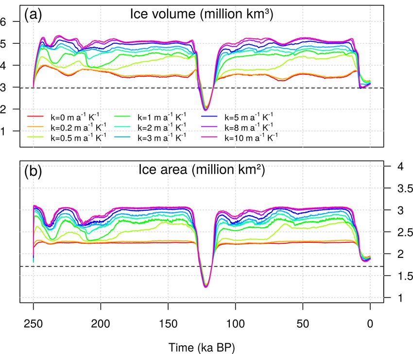
I. Tabone et al.: The sensitivity of the Greenland Ice Sheet                                                                            459

Table 1. Summary of all parameter values used to perturb the basal melting rate equation (Eq. 10) in each sensitivity test.

                    Sensitivity to           Perturbed parameters     Units                                          Values
                    Reference submarine      Bref                     m a−1          0, 0.2, 0.5, 1, 3, 5, 8, 10, 20, 30, 40
                    melting Bref             κ                        m a−1 K−1                                            0
                    Heat-flux                Bref                     m a−1          0, 0.2, 0.5, 1, 3, 5, 8, 10, 20, 30, 40
                    coefficient κ            κ                        m a−1 K−1                0, 0.2, 0.5, 1, 2, 3, 5, 8, 10

2.4   Experimental design

To study how oceanic changes impact the evolution of the
GrIS over the last glacial cycles, we performed a set of sen-
sitivity tests by perturbing the two key parameters of the
basal melting rate equation (Eq. 10): the estimated present-
day submarine melting Bref and the heat-flux coefficient κ.
For each experiment, we ran an ensemble of simulations over
the GrIS domain throughout the last 250 ka. In this study,
the model is initialised with the present-day Greenland to-
pography (Bamber et al., 2013), the characteristic relaxation
time for the lithosphere is set to 3000 years, and the model is
forced by the past relative sea-level reconstruction of Grant
et al. (2014). The first ∼ 100 ka of the simulation are con-
sidered as a spin-up and are not analysed. A summary of all
the parameter values used in each sensitivity test is shown in
Table 1.
   First, we analyse the sensitivity of the model to different           Figure 2. Time evolution of (a) grounded ice volume (million km3 )
constant (in space and time) Bref values applied at the base             and (b) ice-covered area (million km2 ) simulated for different val-
of the ice-sheet marine margins. Due to the scarcity of sub-             ues of Bref (m a−1 ) having set κ = 0 (see Table 1). Dashed lines
marine melt observations along the GrIS coasts, and since                show the present-day estimated volume and area of the GrIS (Bam-
the only available estimates have focused on few very rapid              ber et al., 2013).
tidewater Greenland glaciers that cannot be representative of
the basal melt rate for the entirety of GrIS marine areas (Rig-
not et al., 2010; Motyka et al., 2011; Straneo et al., 2012; Xu          on many factors, such as the water salinity, the depth, the
et al., 2013; Enderlin and Howat, 2013; Fried et al., 2015;              conformation of the cavity, the water velocity below the ice
Rignot et al., 2016; Wilson et al., 2017), we assume present-            shelf and subglacial discharge. The sensitivity test for κ is
day basal melting rates for Greenland comparable to those                firstly done for Bref = 1 m a−1 and then for other Bref values
from Antarctic ice shelves (Rignot et al., 2013). The range of           to show that the GrIS response to the melting rate sensitiv-
values of Bref is set between 0 and 40 m a−1 , while κ is set            ity κ depends on the chosen reference basal melting rate (see
to zero to make the ocean contribution constant in time. The             Table 1).
resulting basal melting rate is thus equal to the tested Bref
value and a condition of no oceanic basal melting around the             3    Results
GrIS is achieved only when both Bref and κ are set to zero.
   Second, we study the sensitivity of the GrIS to the basal             In this section, we present the results of each sensitivity study
melt rate sensitivity κ at the ice–ocean interface. The range of         aiming to assess the impact of the ocean on the evolution of
tested values for κ is between 0 (expressing a temporally con-           the GrIS throughout the last two glacial cycles, especially fo-
stant basal melting rate) and 10 m a−1 K−1 . The choice of this          cusing on the LIG, the LGM and the PD GrIS. The present
range reflects the inference made in Antarctica by Rignot and            work involved a total of 110 model simulations, although
Jacobs (2002) that a variation of 1 K in the effective oceanic           only the most representative cases for each sensitivity study
temperature changes the melt rate by 10 m a−1 (Eq. 6). Due               are discussed.
to the lack of data for Greenland, as a first approximation,
we can assume such a value is also realistic there. This is
surely a simplification of the problem, as the relation between
ocean temperature and melt rate is not universal but depends

www.clim-past.net/14/455/2018/                                                                              Clim. Past, 14, 455–472, 2018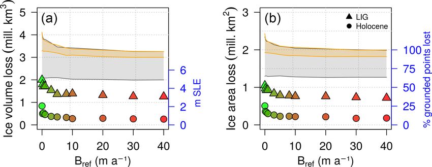
460                                                                     I. Tabone et al.: The sensitivity of the Greenland Ice Sheet

Figure 3. Glacial maximum GrIS surface elevation (km) simulated at Termination II (a–c) and Termination I (d–f) for different values of the
reference basal melting rate (Bref = 0, 5, 10 m a−1 ) under constant oceanic conditions (κ = 0). The timing at which the ice volume reaches
its maximum value during a glacial cycle depends on the experiment and is stated in black for each snapshot. Blue lines indicate the GrIS
extension at the following peak of deglaciation with its corresponding timing reported in blue. Red zones represent the ice shelves extending
beyond the glacial maximum grounding line (black line). Black circles indicate the locations of the Camp Century, NEEM, NGRIP, GRIP
and Dye3 ice cores (from north to south).

3.1   Sensitivity to the reference submarine melting                     limited by the topography of the Greenland itself. Thus, the
                                                                         retreat is almost entirely driven by the surface ablation and
In this experiment, the maximum ice volume reached                       the elevation–melt feedback. For low Bref values, the ice lost
in glacial times ranges between 3.4 and 4.3 million km3                  in a deglaciation is to a large extent determined by the GrIS
(Fig. 2), 15–45 % higher than the observed current value                 configuration in the preceding glacial. As high basal melting
(Bamber et al., 2013), suggesting that under constant oceanic            rates inhibit the ice growth during the cold phase, the higher
forcing, the GrIS is limited to a configuration close to that of         the Bref is applied to the marine margins, the lower ice loss
the present day (Fig. 3). The highest glacial ice volume is              is simulated in the following interglacial (Fig. 4). However,
reached by imposing a null basal melting to the GrIS mar-                for Bref = 5 m a−1 , ice loss becomes insensitive to the melt-
gins (Bref = 0), which corresponds to a simulation forced                ing applied, since the GrIS is also totally land based during
solely by palaeo-atmospheric variations. The varying SMB                 glacial periods and any subsequent ice mass loss is therefore
throughout the cycles still results in a changing GrIS ice vol-          uniquely driven by ablation (compare Fig. 3a and b or Fig. 3d
ume over time. However, during glacials, most grounded ice               and e).
remains on land above sea level, and only small ice shelves
are able to grow (Fig. 3a, d).                                           3.2   Sensitivity to the heat-flux coefficient
   For Bref > 0, a positive basal melt rate is applied to the ma-
rine margins of the whole GrIS throughout the two glacial cy-            We next study the sensitivity to the ocean for a fixed Bref
cles. The submarine melting not only inhibits the grounding-             value of 1 m a−1 (Fig. 5). This value is within present-
line advance during the glacials but contributes to thinning             day submarine melting rates estimates, between those found
the few marine-terminating glaciers still present, constrain-            in the largest remaining outlet glaciers in Greenland (Wil-
ing the grounding line further inland and resulting in a                 son et al., 2017) and those of smaller marine-terminating
GrIS extent close to the observed present-day configuration              glaciers with presumably much lower ocean-induced melt.
(Fig. 3b, c, e, f). This mechanism can still be quite active dur-        Under this assumption, the maximum ice volume simulated
ing glacial times, such that the ice volume can be even lower            in both glacial periods for different κ values ranges be-
than that simulated at the present (Fig. 2). Note that the ice           tween 4 and 5.4 million km3 , greatly exceeding the range
volume is more sensitive to Bref during the glacial periods,             found for the case with constant oceanic forcing. Prescrib-
as during the interglacial periods the effect of the ocean is            ing positive or zero uniform submarine melting to the marine

Clim. Past, 14, 455–472, 2018                                                                          www.clim-past.net/14/455/2018/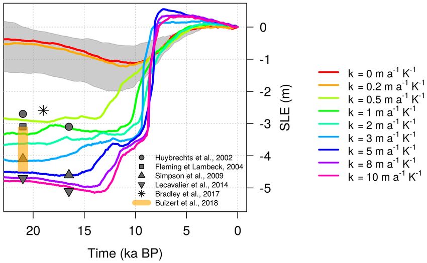
I. Tabone et al.: The sensitivity of the Greenland Ice Sheet                                                                            461

Figure 4. Distribution of the ice volume (a) and area (b) lost dur-
ing the LIG (triangles) and the Holocene (circles) as a function of
Bref . Grey and yellow shades show the range between the maximum
glacial and the minimum interglacial ice volumes (area) for LIG and
Holocene, respectively. The loss is calculated between the time at
which the ice volume reaches its maximum value simulated before
the deglaciation (between 132 and 128 ka BP for TII and between
13 and 9 ka BP for TI) and its following ice minimum (between 122
and 121 ka BP for the Eemian and between 8 and 0 ka BP for the
Holocene). The colours of the points follow the legend of Fig. 2
for clarity. Each ice volume loss has been converted to value of       Figure 5. (a) Time evolution of GrIS grounded ice volume
sea-level-equivalent anomaly (m s.l.e. with respect to its simulated   (million km3 ) and (b) ice area (million km2 ) simulated for differ-
present-day volume.                                                    ent values of the heat-flux coefficient κ, having set Bref = 1 m a−1 .
                                                                       Dashed lines shows the GrIS ice volume and area estimated for the
                                                                       present day (Bamber et al., 2013).
boundaries limits the glacial expansion of the GrIS (Figs. 6a
and 7a), as discussed in Sect. 3.1. Conversely, by intensi-
fying the oceanic forcing applied to the margins (with in-             with preceding glacial GrIS configurations which present a
creasing values of κ), the glacial ice volume increases. For           grounding-line expansion to the continental shelf break. The
κ = 1 m a−1 K−1 , the model simulates a GrIS glacial expan-            slightly increasing ice loss still observed for higher oceanic
sion to the continental shelf break in which the grounding             sensitivities is mostly related to the ice lost in the GrIS inte-
line has already advanced from the present-day continental             riors due to the positive elevation–melt feedback.
boundaries, and large ice shelves are generated in the eastern            Due to our melting parameterization (Eq. 10) and to the
GrIS, especially in the northeast (Figs. 6b and 7b). The max-          Bref value chosen, water below the ice shelves is allowed
imum expansion is simulated for the last glaciation, where             to freeze for κ > 0.5 m a−1 K−1 , favouring ice growth and
the grounding line has almost reached the continental shelf            GrIS expansion (Fig. 5). Below this threshold, the model
break and large ice shelves in the east cover the remaining            still allows for submarine melting rates across the margins in
shallower zones of the bathymetry. For κ = 10 m a−1 K−1 ,              glacial times and the GrIS expansion is almost totally driven
the GrIS extends all the way to the continental shelf break            by surface accumulation. However, the sensitivity with re-
at its glacial maximum, while only a few small floating ice            spect to κ strictly depends on the value of Bref , as it defines
shelves are present (Figs. 6c and 7c).                                 the positive threshold that the glacial GrIS has to overcome
   A larger ice sheet loses more ice during a deglaciation,            to start reacting to the oceanic forcing imposed at the margins
leading to an interglacial state that is almost independent            (Fig. 9). For Bref = 10 m a−1 , the GrIS responds to the ocean
of κ (Fig. 5). This response is related to the saturation of           only for κ > 3 m a−1 K−1 , while for Bref = 30 m a−1 the GrIS
the oceanic forcing in warm peaks, when the GrIS is al-                starts to expand only for κ > 8 m a−1 K−1 . For high Bref ,
most totally land-based and the ice loss is hence mostly               since a constant high submarine melting is applied overall,
due to the increase in atmospheric temperature and precip-             the glacial GrIS is almost constrained to the PD configura-
itation. Since glacial accretion affects the ice growth much           tion and exposure to the ocean is reduced. Only a sufficiently
more than basal melting during the retreat, the ice loss dur-          high κ to counteract this strong melting is able to make the
ing a deglaciation monotonically increases with increasing             GrIS expand and then retreat during the interglacial. Once
κ (Fig. 8). Thus, for larger κ values, more ice grows dur-             the reaction has started, the sensitivity of the GrIS to κ in-
ing glacial periods and more ice is lost, and faster, during           creases with increasing Bref ; i.e. small variations in the mag-
the subsequent deglaciation. Mass loss is mostly due to the            nitude of κ lead to a fast and large growth of ice during
large number of grounded-ice zones that are converted into             glacials and consequently to a fast and large loss of ice dur-
ice-free areas during the deglaciation (Fig. 8b). The percent-         ing the deglaciation. Similar results are found for the LIG
age of grounded points lost until the peak of an interglacial          (not shown).
period saturates for κ above 3 m a−1 K−1 in correspondence

www.clim-past.net/14/455/2018/                                                                          Clim. Past, 14, 455–472, 2018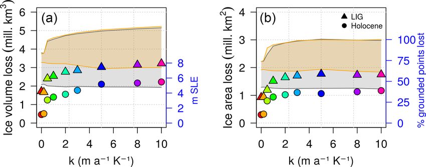
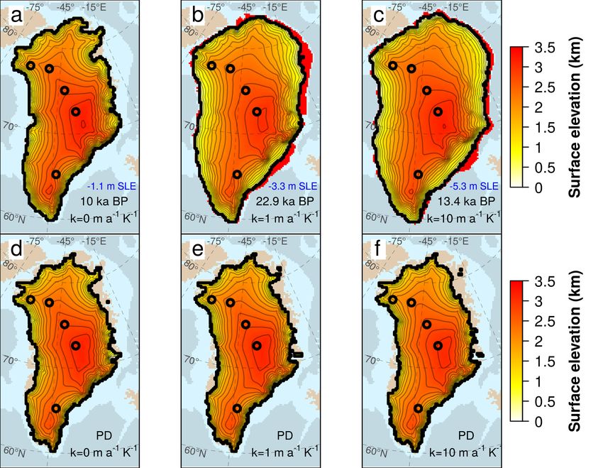
462                                                                      I. Tabone et al.: The sensitivity of the Greenland Ice Sheet

Figure 6. GrIS surface elevation (km) simulated at the penultimate glacial maximum (TII) (a–c) and at the LIG minimum (Eemian) (d–f)
for three values of the melting rate sensitivity κ having set Bref = 1 m a−1 . The timing of these snapshots depends on the experiment and is
stated in black for each snapshot. Corresponding ice volume (in s.l.e.) is shown in blue. Red zones represent the ice shelves extending beyond
the glacial maximum grounding line (black line). Black circles indicate the locations of the Camp Century, NEEM, NGRIP, GRIP and Dye3
ice cores (from north to south).

Figure 7. GrIS surface elevation (km) simulated at the LGM (TI) (a–c) and present-day GrIS (d–f) for three values of the heat-flux coefficient
κ having set Bref = 1 m a−1 . The timing of the snapshots depends on the experiment and is stated in black for each snapshot. Corresponding
ice volume (in s.l.e.) is shown in blue. Red zones represent the ice shelves extending beyond the LGM grounding line (black line). Black
circles indicate the locations of the Camp Century, NEEM, NGRIP, GRIP and Dye3 ice cores (from north to south).

Clim. Past, 14, 455–472, 2018                                                                           www.clim-past.net/14/455/2018/
I. Tabone et al.: The sensitivity of the Greenland Ice Sheet 463
Figure 8. Distribution of ice volume (a) and area (b) lost during
the LIG and the Holocene as a function of κ, for Bref = 1 m a−1 .
Grey and yellow shades show the deviation between the maximum Figure 9. Distribution of the ice volume lost in the Holocene
and the minimum ice volumes (area) for LIG and Holocene, re- as a function of the heat-flux coefficient κ, simulated for three
spectively (see Fig. 5). The loss is calculated between the time at selected reference basal melting rates (Bref = 1 m a−1 in green,
which the ice volume reaches its maximum value simulated before Bref = 10 m a−1 in blue and Bref = 30 m a−1 in red). The ice vol-
deglaciation (between 140 and 128 ka BP for TII and between 19 ume loss is calculated between the time at which the ice volume
and 10 ka BP for TI) and the subsequent ice minimum (between reaches its maximum value before the deglaciation and the present
122 and 121 ka BP for the Eemian and between 8 and 0 ka BP for day. The green points are the same as the circles of Fig. 8a (for the
the Holocene). The colours of the points follow the legend of Fig. 5 Holocene).
for clarity.
suggested by some previous studies (e.g. 1.2–3.5 m s.l.e. for
3.3 Last interglacial Helsen et al. (2013), 0.4–4.4 m s.l.e. for Robinson et al.
(2011) and 0.4–3.8 m s.l.e. for Stone et al., 2013). Also, the
The amount of ice lost during the LIG period increases timing at which the peak of deglaciation occurs, which spans
with the oceanic sensitivity κ. High κ values lead to higher between 122.3 and 121.6 ka BP in all the simulations, agrees
glacial ice volumes and to larger ice losses during the con- with the timing proposed in many previous studies (Calov
sequent deglaciation (Fig. 8). The range of observed volume et al., 2015; Langebroek and Nisancioglu, 2016; Robinson
changes spans between 4.2 m s.l.e. (for κ = 0) and 8 m s.l.e. et al., 2011; Stone et al., 2013; Yau et al., 2016). The time
(for κ = 10 m a−1 K−1 ), above the present-day GrIS ice vol- at which the peak of the Eemian occurs in our experiments
ume. Despite this large ice-loss range, all GrIS configurations depends partly on the timing of the atmospheric tempera-
simulated at the LIG ice minimum (Eemian) present a similar ture peak and partly on the duration of the post-glacial re-
extension (Fig. 6d–f). In all experiments, a large retreat is ob- bound, which controls the intrusion of warm waters into the
served in the north (especially in the northeast), where melt- GrIS bays enhancing the ocean-driven retreat. However, the
ing overcomes the low accumulation rates, and in the south- Eemian peak does not depend on the maximum insolation
west, where the ice discharge from the interior is enhanced since the PDD scheme used does not account for past insola-
by the presence of fast ice streams and, in some areas, by the tion changes.
fact that the bedrock is below sea level. Although the position
of the land-ice borders at the Eemian is not very sensitive to 3.4 Last Glacial Maximum
κ, the corresponding surface elevation fields show some dif-
ferences depending on κ. For high values of κ, a lower ice Although many uncertainties about the GrIS configura-
elevation is simulated over the GrIS (compare Fig. 6d and f), tion during the last glacial period still exist, several esti-
a tendency that is reflected in a slightly lower ice volume too mates of the sea-level contribution from the GrIS during the
(Fig. 5). last deglaciation can be found in the literature: 2.6 m s.l.e.
It is interesting to note that even when imposing a very (Bradley et al., 2017), 2.7 m s.l.e. (Huybrechts, 2002), be-
high κ, the complete disappearance of the GrIS is not sim- tween 2 and 3 m s.l.e. (Clark and Mix, 2002), 3.1 m s.l.e.
ulated. The GrIS is only partly deglaciated and all ice-core (Fleming and Lambeck, 2004), 4.1 m s.l.e. (Simpson et al.,
sites are still covered by ice (including the discussed ice core 2009), between 3.1 and 4.5 m s.l.e. (Buizert et al., 2018) and
locations of Dye3 and NEEM). Since the oceanic-driven re- 4.7 m s.l.e. (Lecavalier et al., 2014). These estimates come
treat is limited by the land-based configuration observed in from ice-sheet models of different complexity, with their own
the interglacials, the retreat during the LIG is mainly con- dynamics and boundary conditions. Particularly the ice-sheet
trolled by the atmospheric temperatures and precipitations model used by Simpson et al. (2009) and Lecavalier et al.
with which the model is forced. (2014) is run in combination with a GIA and RSL model
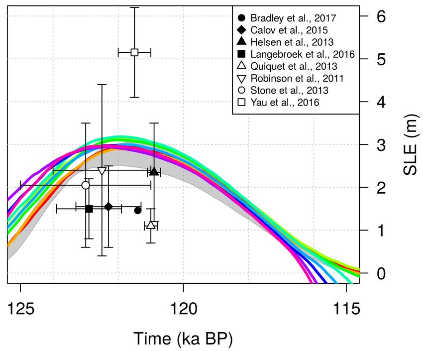
The amount of ice lost during the Eemian relative to and then constrained by past surface elevations derived from
the present day (Fig. 10), which ranges between 2.9 and ice-core data, observations of past changes in RSL and the
3.2 m s.l.e., is within the uncertainty range of ice volumes present-day GrIS configuration. These models do not solve
www.clim-past.net/14/455/2018/ Clim. Past, 14, 455–472, 2018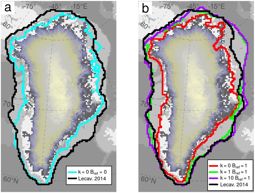
464                                                                       I. Tabone et al.: The sensitivity of the Greenland Ice Sheet

                                                                          Figure 11. GrIS ice volume evolution simulated for different val-
Figure 10. GrIS ice volume evolution simulated for different val-         ues of the melting rate sensitivity κ during the last deglaciation. The
ues of the melting rate sensitivity κ during the last interglacial (see   ice volumes have been converted to values of s.l.e. anomaly with
Fig. 5 for the line colour legend). The ice volumes have been con-        respect to the present-day volumes estimated in each specific sim-
verted to values of s.l.e. anomaly with respect to the present-day        ulation. As in Fig. 10, grey shading represents the simulations for
volumes estimated in each specific simulation. Grey shading rep-          the different reference basal melting rates (Bref ) investigated for the
resents the reference basal melting rates Bref investigated for the       case of constant-in-time oceanic forcing (κ = 0). The upper bound
case of constant-in-time oceanic forcing (κ = 0 m a−1 K−1 ). The          refers to Bref = 40 m a−1 and the lower bound to Bref = 0 m a−1 .
upper bound refers to Bref = 40 m a−1 and the lower bound to              Grey dots and orange shading indicate estimates of the GrIS ice
Bref = 0 m a−1 . Black and white symbols indicate the LIG mini-           volume at the LGM (21 ka BP) and at the maximum ice volume
mum ice volumes estimated by previous studies. The tight clus-            reached before the last deglaciation (16.5 ka BP), as suggested by
tering of our estimates compared to previous work is due to the           previous work.
fact that the sole uncertainty is here related to the oceanic forcing
through κ.
                                                                          than the LGM volumes of Simpson et al. (2009) and Lecav-
                                                                          alier et al. (2014) (Fig. 11), since only with κ > 3 m a−1 K−1
the dynamics of the ice shelves or the grounding-line migra-
                                                                          does the model simulate a maximum ice volume compara-
tion, which is parameterized. However, their estimates of the
                                                                          ble to those ranges. The discrepancy in volumes, despite the
GrIS spatial extent can be considered as the most realistic
                                                                          same extension, could be related to the different dynamics
reconstructions of the recent past glacial GrIS so far.
                                                                          and boundary conditions applied in the two models. Never-
   Under constant oceanic conditions, the LGM-PD ice ex-
                                                                          theless, our simulated ice volumes are in agreement with re-
cess simulated by our model at 21 kyr BP spans between
                                                                          cent estimates corrected for seasonal surface air temperatures
0 and 1.4 m s.l.e. for Bref ranging from 0 to 40 m a−1 , in-
                                                                          in Greenland during the LGM (Buizert et al., 2018).
creasing with decreasing Bref values (grey shaded region –
                                                                             The timing of the reconstructed deglaciation can also pro-
Fig. 11). This range is well below previous LGM ice volume
                                                                          vide information for comparison. The maximum increases
reconstructions found in the literature (grey points). How-
                                                                          suggested by Simpson et al. (2009) (4.6 m s.l.e.) and Lecav-
ever, slightly larger ice volumes (0.6–2 m s.l.e.) are found at
                                                                          alier et al. (2014) (5.1 m s.l.e.) occur at 16.5 ka BP, while our
the peak simulated further in time in the glaciation (∼ 13–
                                                                          simulations suggest a timing dependent on κ ranging from
10 ka BP). For the case with no submarine melting (Bref =
                                                                          20 to 10 ka BP for very low κ values (Fig. 11). The mag-
0 m a−1 ), the maximum ice volume (lower bound of grey
                                                                          nitudes of the oceanic sensitivity that best approximate the
shadow, at ∼ 12 kyr BP) is close to those of Huybrechts
                                                                          evolution of the GrIS before the Holocene are thus between
(2002) and Bradley et al. (2017). In this simulation, the GrIS
                                                                          5 m a−1 K−1 (4.6 m s.l.e. at 17.4 ka BP) and 10 m a−1 K−1
increases moderately as its extension surpasses its PD bor-
                                                                          (5.3 m s.l.e. at 14 ka BP). However, some discrepancies be-
ders and the grounding line approaches the continental shelf
                                                                          tween our GrIS glacial extension and that of Lecavalier et al.
(Fig. 12a). Nevertheless, the atmospheric forcing alone is not
                                                                          (2014) are still present (Fig. 12b).
sufficient to make the GrIS expand as expected during the
LGM. According to reconstructions, the GrIS extended as
far as the continental shelf break in every direction, except in          3.5   Present-day GrIS
the northeast region where the grounding line remains closer
to the coast (Lecavalier et al., 2014). In our simulations, the           Given that the topography of the present-day GrIS is one of
GrIS reaches a glacial expansion consistent with the litera-              the trustworthy measures used to assess the reliability of an
ture only for κ ≥ 1 m a−1 K−1 (Fig. 12b). However, the ice                ice-sheet model, we compare our present-day GrIS ice thick-
volume reached for this oceanic sensitivity is still smaller              ness and extent simulated for κ = 10 m a−1 K−1 to those es-

Clim. Past, 14, 455–472, 2018                                                                            www.clim-past.net/14/455/2018/
I. Tabone et al.: The sensitivity of the Greenland Ice Sheet 465
Figure 12. GrIS total extent (ice shelves are included) simulated
Figure 13. Modelled minus observed surface elevation for the
at the peak of the last glaciation for (a) no melting/freezing at the
present day. Modelled data are taken from the GRISLI-UCM sim-
grounding line (cyan) and (b) κ = 0, 1 and 10 m a−1 K−1 (red,
ulation which best estimates the presumed LGM extension (Bref =
green and purple lines, respectively) for Bref = 1 m a−1 . The tim-
1 m a−1 and κ = 10 m a−1 K−1 ) while the observed surface eleva-
ing of the glacial maximums is (a) 12 kyr BP and (b) 10, 20 and
tion is taken from Bamber et al. (2013). Purple and black lines rep-
14 kyr BP for κ = 0, 1 and 10 m a−1 , respectively. LGM (21 kyr BP)
resent simulated and observed GrIS extensions, respectively. Black
GrIS grounding-line position estimated by Lecavalier et al. (2014)
circles indicate the locations of the Camp Century, NEEM, NGRIP,
is shown for comparison (black line).
GRIP and Dye3 ice cores (from north to south).
timated by Bamber et al. (2013) (Fig. 13). The choice of this
4 Discussion
particular κ value is based on the discussion above (Sect. 3.4)
for the LGM and is supported by the good agreement be-
Our model simulates the advance and retreat of the GrIS dur-
tween the simulated present-day ice volume and observa-
ing the last two glacial cycles. Transient simulations reflect
tions (Bamber et al., 2013) (Fig. 7f). The simulated extent
the ice-sheet response to the specific oceanic forcing applied
of the GrIS matches reasonably well the observations. How-
to the model. This reaction is different for glacial and inter-
ever, notable discrepancies are observed in some sectors. The
glacial periods (Fig. 5). Since during the interglacial peri-
main differences are found in the northeast, where GRISLI-
ods the GrIS is almost totally land based and therefore less
UCM predicts an ice margin somewhat too far inland, and
exposed to the ocean, the minimum ice volume reflects the
in the southwest, where our model is not able to make the
oceanic imprint only mildly and is limited to a small range
GrIS retreat as expected. The ice loss in the north is a known
of possible values. On the other hand, the volume reached
problem that appears in many studies when simulating the
in glacial periods is much more sensitive to κ. Although the
GrIS during an interglacial (Stone et al., 2010; Born and Ni-
maximum ice volume loss is constrained by the imposed lim-
sancioglu, 2012). In the interior, the difference in ice thick-
ited extension to the continental shelf break, the large ice loss
ness is relatively low. However, the GrIS simulated by our
observed for a high oceanic sensitivity is closely related to
model generally shows thicker ice along the margins, a ten-
the GrIS configuration in the previous glacial, which is essen-
dency that propagates inland. Other areas in which our sim-
tially marine-based at the margins and therefore more sub-
ulated ice thickness is lower than that observed are located
jected to oceanic changes (Fig. 6c). As water temperatures
in the centre of the continent and in the very southeast corre-
rise at the beginning of the deglaciation, the basal melting
sponding to a mountainous region. However, the focus of our
rate increases too (Eq. 10), thinning ice shelves at the bound-
work is not to exactly reproduce the observed present-day
aries, enhancing outflow of ice and triggering grounding-line
GrIS ice volume at the end of the simulations but rather to
retreat. The effects of this ocean-driven retreat are not lo-
demonstrate the impact of the ocean on the GrIS past evolu-
cally confined but are propagated inland through a dynamic
tion. From this perspective, the simulations arrive at a reason-
response of the grounded ice sheet. The ice loss at the mar-
able representation of the present day and within the range of
gins triggers ice advection from the interior which further
other models.
increases the ice discharge into the ocean, and, as the thick-
ness of the inland ice decreases, the elevation–melt feedback
begins. At a given stage of the deglaciation, when the whole
ice sheet starts to become land based, this atmosphere-driven
www.clim-past.net/14/455/2018/ Clim. Past, 14, 455–472, 2018466 I. Tabone et al.: The sensitivity of the Greenland Ice Sheet retreat becomes the sole driver of ice mass loss. The simu- and ocean. In principle, forcing the ocean with an index de- lated retreat during this phase is influenced by the choice of rived from past ocean temperatures could be more appropri- the surface melt scheme used in the model. At the peak of the ate. To this end, we ran additional simulations by applying Eemian, the melt determined by the PDD scheme can be 20– the multiproxy index α for the atmosphere and another in- 50 % lower than the melt calculated if past insolation changes dex for the ocean calculated from benthic-retrieved ocean are taken into account (Robinson and Goelzer, 2014). This temperatures (Waelbroeck et al., 2002). The results of the inaccuracy therefore influences the GrIS contributions to sea- new simulations show very little differences from the ones level rise for the last interglacial (Fig. 10), which could be reported here, while the same sensitivity to the ocean is pre- underestimated. served (not shown). Thus, such a distinction in forcing does As discussed in Sect. 3.4 and 3.5, the oceanic forcing that not affect the main outcomes of this work. seems to best reconstruct the past (LGM) and the present Our results may well be model dependent, and some GrIS is achieved for a heat-flux coefficient of 10 m a−1 K−1 . model limitations should be noted. As described in Sect. 2.1, However, the submarine melt scheme used and some sim- our ice-sheet–shelf model is provided with an internal GIA plifications made in its treatment may partly influence our scheme which accounts for bedrock deformation due to results. Firstly, only a limited range of reference submarine changes in the GrIS ice load. However, since the GrIS rests melting rates has been investigated, since only two of the on the peripheral forebulge of the North American ice sheets system model parameters have been explored (Table 1). Sec- (NAIS), such as the Laurentide Ice Sheet, variations in the ondly, our melting parameterization is highly conditioned by NAIS ice load induce consequent vertical motions of the the Bref value assumed to represent the present-day subma- lithosphere beneath the GrIS (Lecavalier et al., 2014). The rine melting rate around the GrIS (Fig. 8), as it consequently resulting GrIS isostatic adjustment is therefore the combi- determines the minimum κ value needed to allow the GrIS nation of these local and non-local responses which make to respond to the ocean (Fig. 3). Using a single value for this the GIA treatment rather complex. In principle, these non- term is a coarse approximation to reality, but since the de- local effects should be taken into account as they contribute tailed distribution of the present-day sub-shelf melt along the to the sea-level variability, becoming especially relevant at coasts does not yet exist for Greenland, the retrieval of a 2-D the beginning of deglaciations when the ice mass loss is sig- field would be complex and highly uncertain. However, we nificantly induced by sea-level rise (Lecavalier et al., 2017). have considered the same order of magnitude of melt rates as However, for the sake of simplicity, the GrIS isostatic ad- is proposed in the literature for the AIS, which spans values justment is assumed here to be only due to local ice mass from negative to above 40 m a−1 in some very active regions variations, as other works have done in the past (Greve and (Rignot and Jacobs, 2002). In support of this evidence, simi- Blatter, 2009; Helsen et al., 2013; Huybrechts, 2002; Lange- lar basal melting rates have been found recently in some GrIS broek and Nisancioglu, 2016; Stone et al., 2013). ice tongues (Wilson et al., 2017). Thirdly, the basal melt- The simulated ice volume at the present day is overesti- ing equation strongly depends on the oceanic temperature mated for all investigated values of κ (Fig. 8). This fact sug- anomaly TLGM,ocn − TPD, ocn , which has been prescribed to a gests that our model has a tendency to overestimate the ice spatially constant value of −3 K. Since this term impacts the thickness of the GrIS, especially in the marginal zones of oceanic sensitivity through κ (Eq. 10), it is clear that the same the domain, a well-known phenomenon (Calov et al., 2015). results obtained in this work would have been reached by These discrepancies are partly linked to the relatively low fixing one value of κ and instead examining the influence of model resolution (20 km × 20 km), which limits the accu- different levels of the 1Tocn on the GrIS past evolution. Con- racy in estimating the margins especially along the fjords, sidering a spatially constant SST anomaly represents an ide- and partly due to the boundary conditions applied to the ice- alized simplification of the oceanic forcing for two reasons: sheet model, such as the basal sliding. The coarse model res- the temperature of the water is clearly not uniform along the olution prevents the model from resolving fine-scale phys- GrIS coasts and the melt at the grounding line is presumably ical processes at the marine-terminating outlet glaciers that controlled by water temperature deeper in the ocean column end in narrow fjords, although they are considered as the pri- (between 100 and 1000 m in Greenland; Rignot et al., 2016). mary sources of ice discharge today due to oceanic changes. These issues could be avoided, for example, by using spa- Such an inability of our model may be more relevant when tially variable (horizontally and vertically) oceanic temper- modelling the GrIS retreat during the LIG and the Holocene. atures from available model outputs for Greenland. To see The lack of a sub-grid fjord treatment does not allow for a whether this simplification could influence our results, some proper analysis of the ice front processes which become rel- tests using 2-D temperatures from CLIMBER-3α snapshots evant when the retreat has reached the continental area above (Montoya and Levermann, 2008) have been run (not shown). the sea level. Especially when, as in our case, the submarine Despite some differences in the ice distribution and the time melt goes abruptly to a high value at the grounding line, the of the retreat, the main results obtained in this work did implementation of a sub-grid-scale parameterization would not change. Finally, another simplification made here is the allow the small processes at the fjords to be accurately re- assignation of the same climatic index α to both atmosphere solved (Calov et al., 2015; Favier et al., 2016; Gladstone Clim. Past, 14, 455–472, 2018 www.clim-past.net/14/455/2018/
I. Tabone et al.: The sensitivity of the Greenland Ice Sheet                                                                      467

et al., 2017). However, these limitations lead to only second-       for global effects. These discrepancies are probably due not
order effects given the scope of our work.                           only to the different submarine melt schemes considered in
   The parameterization used for the submarine melting rate          each model but also to the features of the model dynam-
at the GrIS marine margins is a simplification compared              ics, such as the sliding law and the grounding-line migration
to other temperature-dependent submarine melting schemes.            scheme. Following these assumptions, a sub-grid treatment
We are aware that the melting rate depends on many regional          of the small-scale processes taking place at the grounding
factors such as the temperature and salinity of the ocean at         line, such as basal sliding, sub-shelf melting, hydrology and
the ice-shelf margin, the shape of the ice-shelf cavity and          migration, will be added in our model in the future. This will
the depth of the grounding line, which our equations do not          provide a more realistic description of grounding-line pro-
take into account. However, our simple construction allows           cesses such as the enhanced submarine melting as well as
us to test the sensitivity of the GrIS to the oceanic forcing        the basal drag at the margin of fast grounded ice.
in a straightforward manner and is found to be particularly             We should finally remark that the GrIS evolution during
suitable for palaeo-studies.                                         the last two glacial cycles has been assessed here only from
   Our basal melting scheme is implemented in such a way             an oceanic point of view, while the influence of different at-
that the melting at the grounding line (Eq. 10) is higher than       mospheric forcings has not been investigated. This simplifi-
the one set below the ice shelves (Eq. 11). This approach            cation may be especially important for the results shown for
is supported by sub-shelf melting rate estimates (Dutrieux           the LIG and the Holocene, in which the retreat is mostly in-
et al., 2013; Reese et al., 2017; Rignot and Jacobs, 2002; Wil-      duced by surface ablation. However, this point will be in the
son et al., 2017). Moreover, we assume that the ratio between        scope of future work.
the two is 1 : 10, which is valid for the present day, but could
be inaccurate for glacial times. However, some experiments
done with ratios of 1 : 5 and 1 : 15 differ very little from the     5   Conclusions
results presented in this work (not shown). Therefore, our pa-
rameterization is much less sensitive to the melting rate be-        Here, we assessed the impact of palaeo-oceanic tempera-
low the ice shelves with respect to that at the grounding line.      ture variations on the evolution of the GrIS on a glacial–
On the other hand, a recent study shows the need to make             interglacial timescale. By using a three-dimensional hybrid
the basal melting decrease smoothly to zero when approach-           ice-sheet–shelf model including a parameterization of the
ing the grounding line from the ice shelf to avoid resolution-       basal melting rate at the GrIS marine margins, the model
dependent performances (Gladstone et al., 2017). This can be         simulates the evolution of the whole ice sheet under tem-
achieved, for example, by considering the submarine melt to          porally variable oceanic conditions. Firstly, the magnitude of
be dependent on the water-column thickness beneath the ice           the oceanic forcing applied at the ice–ocean interface triggers
shelf, as Bradley et al. (2017) suggested in their work. It is in-   and drives the grounding-line advance (through water freez-
teresting to compare our results with theirs, as we address the      ing) and retreat (through ice melting). Secondly, it induces
same scientific problem, i.e. the impact of submarine melting        a dynamic adjustment of the grounded ice sheet, determin-
on the evolution of the past GrIS, from two different points         ing the amount of ice grown (lost) during the cold (warm)
of view. Our submarine melt scheme is implicitly a linear            stages. Although the GrIS evolution is a result of the at-
function of the water depth, as, going down through the wa-          mospheric and oceanic forcings operating together, we have
ter column, the melt rate maintains the same value until it          shown that the ocean is a primary driver of the GrIS glacial
reaches a critical zone at which the sub-shelf melt is set to        advance. Not only must the oceanic forcing be activated, but
50 m a−1 to avoid improbable ice expansion (Sect. 2.3). Our          it must be strong enough to reproduce a reliable GrIS evolu-
work shows that without melting/freezing at the grounding            tion throughout the glacial cycles. It is important to remark
line (for Bref = 0 and κ = 0), the GrIS is not able to reach the     that other factors which could affect the GrIS evolution have
continental shelf break (Fig. 12a). However, it is able to ex-       not yet been explored in detail. Sensitivity tests to the atmo-
tend past the present-day coastline, similar to the simulations      spheric forcing, glacial isostatic adjustment effects and spa-
presented by Bradley et al. (2017). Moreover, experiments            tially non-uniform submarine melt rates should be taken into
performed under the same oceanic conditions with increased           account in the future to analyse the scientific problem from a
basal sliding at the margins show that our model allows fur-         broad range of points of view. Nevertheless, we have shown
ther expansion during the glacial periods (not shown). On            that changing oceanic conditions is a fundamental contrib-
the other hand, the model used by Bradley et al. (2017) has          utor to the evolution of the whole GrIS, suggesting that the
the capability of making the GrIS retreat during interglacial        oceanic component should be included as an active forcing
periods only if the submarine meltwater depth relation is ex-        in palaeo-ice-sheet models.
ponential and if RSL variations due to both local and non-
local effects are considered. On the contrary, a proper retreat
during the deglaciations is always achieved in our simula-           Code and data availability. The GRISLI-UCM code and the
tions (Figs. 3 and 6–7), although the GIA does not account           analysed data are available from the authors upon request.

www.clim-past.net/14/455/2018/                                                                      Clim. Past, 14, 455–472, 2018
You can also read