Deciphering anomalous heterogeneous intracellular transport with neural networks - eLife
←
→
Page content transcription
If your browser does not render page correctly, please read the page content below
RESEARCH ARTICLE

                                     Deciphering anomalous heterogeneous
                                     intracellular transport with neural
                                     networks
                                     Daniel Han1,2,3*, Nickolay Korabel1, Runze Chen4, Mark Johnston2,
                                     Anna Gavrilova1,2, Victoria J Allan2*, Sergei Fedotov1*, Thomas A Waigh3,5*
                                     1
                                      Department of Mathematics, University of Manchester, Manchester, United
                                     Kingdom; 2School of Biological Sciences, University of Manchester, Manchester,
                                     United Kingdom; 3Department of Physics and Astronomy, University of Manchester,
                                     Manchester, United Kingdom; 4Department of Computer Science, University of
                                     Manchester, Manchester, United Kingdom; 5The Photon Science Institute, University
                                     of Manchester, Manchester, United Kingdom

                                     Abstract Intracellular transport is predominantly heterogeneous in both time and space,
                                     exhibiting varying non-Brownian behavior. Characterization of this movement through averaging
                                     methods over an ensemble of trajectories or over the course of a single trajectory often fails to
                                     capture this heterogeneity. Here, we developed a deep learning feedforward neural network
                                     trained on fractional Brownian motion, providing a novel, accurate and efficient method for
                                     resolving heterogeneous behavior of intracellular transport in space and time. The neural network
                                     requires significantly fewer data points compared to established methods. This enables robust
*For correspondence:                 estimation of Hurst exponents for very short time series data, making possible direct, dynamic
daniel.han@manchester.ac.uk
                                     segmentation and analysis of experimental tracks of rapidly moving cellular structures such as
(DH);
                                     endosomes and lysosomes. By using this analysis, fractional Brownian motion with a stochastic
viki.allan@manchester.ac.uk (VJA);
                                     Hurst exponent was used to interpret, for the first time, anomalous intracellular dynamics,
sergei.fedotov@manchester.ac.uk
(SF);                                revealing unexpected differences in behavior between closely related endocytic organelles.
t.a.waigh@manchester.ac.uk
(TAW)

Competing interests: The             Introduction
authors declare that no
                                     The majority of transport inside cells on the mesoscale (nm-100mm) is now known to exhibit non-
competing interests exist.
                                     Brownian anomalous behavior (Metzler and Klafter, 2004; Barkai et al., 2012; Waigh, 2014). This
Funding: See page 17                 has wide ranging implications for most of the biochemical reactions inside cells and thus cellular
Received: 26 September 2019          physiology. It is vitally important to be able to quantitatively characterize the dynamics of organelles
Accepted: 22 March 2020              and cellular responses to different biological conditions (van Bergeijk et al., 2015;
Published: 24 March 2020             Patwardhan et al., 2017; Moutaux et al., 2018). Classification of different non-Brownian dynamic
                                     behaviors at various time scales has been crucial to the analysis of intracellular dynamics
Reviewing editor: Robert H
                                     (Fedotov et al., 2018; Bressloff and Newby, 2013), protein crowding in the cell (Banks and Fradin,
Singer, Albert Einstein College
of Medicine, United States           2005; Weiss et al., 2004), microrheology (Waigh, 2005; Waigh, 2016), entangled actin networks
                                     (Amblard et al., 1996), and the movement of lysosomes (Ba et al., 2018) and endosomes (Flores-
   Copyright Han et al. This
                                     Rodriguez et al., 2011). Anomalous transport is currently analyzed by statistical averaging methods
article is distributed under the
                                     and this has been a barrier to understanding the nature of its heterogeneity.
terms of the Creative Commons
                                        Spatiotemporal analysis of intracellular dynamics is often performed by acquiring and tracking
Attribution License, which
permits unrestricted use and         microscopy movies of fluorescing membrane-bound organelles in a cell (Rogers et al., 2007; Flores-
redistribution provided that the     Rodriguez et al., 2011; Chenouard et al., 2014; Zajac et al., 2013). These tracks are then com-
original author and source are       monly interpreted using statistical tools such as the mean square displacement (MSD) averaged over
credited.                            the ensemble of tracks, hDr 2 ðtÞi. The MSD is a measure that is widely used in physics, chemistry and

Han et al. eLife 2020;9:e52224. DOI: https://doi.org/10.7554/eLife.52224                                                              1 of 28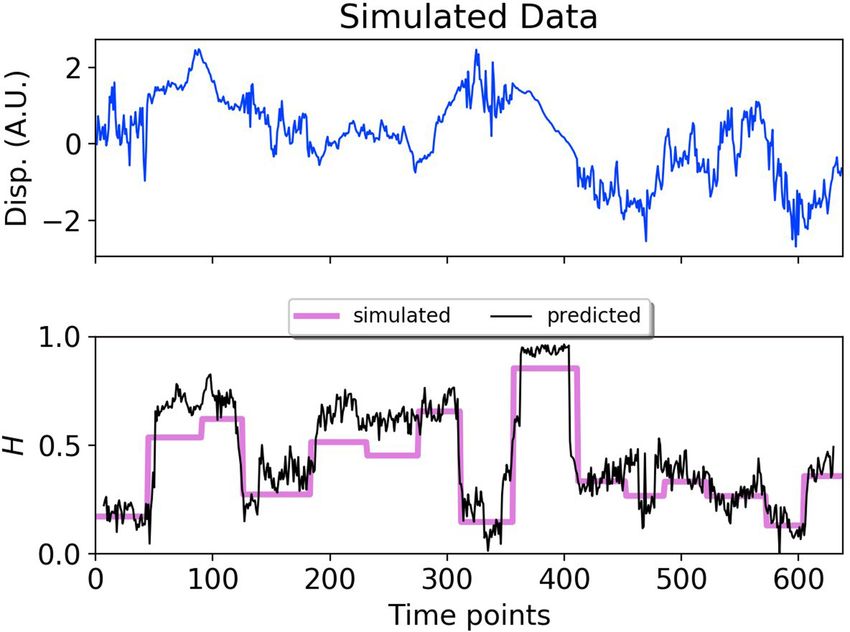
Research article                                                                   Cell Biology Computational and Systems Biology

                                   biology. In particular, MSDs serve to distinguish between anomalous and normal diffusion at differ-
                                   ent temporal scales by determining the anomalous exponent a through hDr 2 ðtÞi ~ t a (Metzler and
                                   Klafter, 2000). Diffusion is defined as a ¼ 1, sub-diffusion 0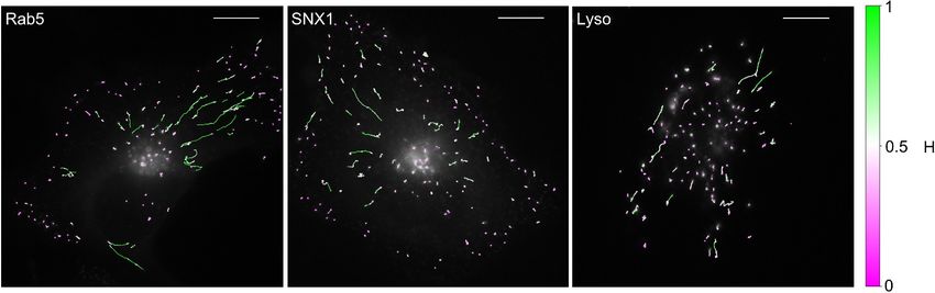
Research article Cell Biology Computational and Systems Biology
a c d
2 RR (σH = 0.154 ) MSD (σH = 0.214) SR (σH = 0.236) DLFNN (σH = 0.057)
Hest
0
2
Hest
0
1 e
0
HΔ
−1
1
0
HΔ
−1
0.0 0.5
Hsim
1.0 0.0 0.5
Hsim
1.0 0.0 0.5
Hsim
1.0 0.0 0.5
Hsim
1.0 f 0.20
Anti-triangle
b 0.15 Triangle
100 Rectangular
MSD σH 0.10
Rescaled Range
σH Sequential Range
Triangular DLFNN 0.05
10−1 Rectangular DLFNN
Anti-triangular DLFNN 0.00 0 1
10 10
Hidden layers
101 102
n
g h i 0.00
b(Hsim)
0.30
1 layer −0.01
0.25 2 layers
3 layers
0.20 0.2
Var(Hsim)
7 layers
σH 0.15 12 layers
σH 0.0005
0.0000
0.10 0.1
0.001
0.05
MSE
0.00 0.0 0.2 0.4 0.6 0.8 1.0
0.000
0 20 40 60 Noise 0.0 0.2 0.4 0.6 0.8 1.0
nrand
. Signal Hsim
Figure 1. Tests of exponent estimation for the DLFNN using N = 104 simulated fBm trajectories. (a) Plots showing the Hurst exponent estimates of fBm
trajectories with n ¼ 102 data points by a triangular DLFNN with three hidden layers compared with conventional methods. Plots are vertically grouped
by Hurst exponent estimation method: (left to right) rescaled range, MSD, sequential range and DLFNN. sH values are shown in the title. Top row:
Scatter plots of estimated Hurst exponents Hest and the true value of Hurst exponents from simulation Hsim . The red line shows perfect estimation.
Second row: Due to the density of points, a Gaussian kernel density estimation was made of the plots in the top row (see Materials and methods). Third
row: Scatter plots of the difference between the true value of Hurst exponents from simulation and estimated Hurst exponent DH ¼ Hsim Hest . Last
row: Gaussian kernel density estimation of the plots in the third row. (b) sH as a function of the number of consecutive fBm trajectory data points n for
different methods of exponent estimation. Example structures for two hidden layers and n ¼ 5 time series input points of the anti-triangular, rectangular
and triangular DLFNN are shown in (c, d and e), respectively. (f) sH as a function of the number of hidden layers in the DLFNN for triangular,
rectangular and anti-triangular structures. (g) sH as a function of the number of randomly sampled fBm trajectory data points nrand with different number
Noise
of hidden layers in the DLFNN shown in the legend. (h) sH as a function of the noise-to-signal ratio (Signal) (NSR) from Gaussian random numbers added
to all n ¼ 102 data points in simulated fBm trajectories. (i) Plots of bias bðHsim Þ, variance VarðHsim Þ and mean square error (MSE) as functions of Hsim . For
each value of Hsim , fBm trajectories with n ¼ 100 points were simulated and estimated by a triangular DLFNN.
Han et al. eLife 2020;9:e52224. DOI: https://doi.org/10.7554/eLife.52224 3 of 28
Research article Cell Biology Computational and Systems Biology
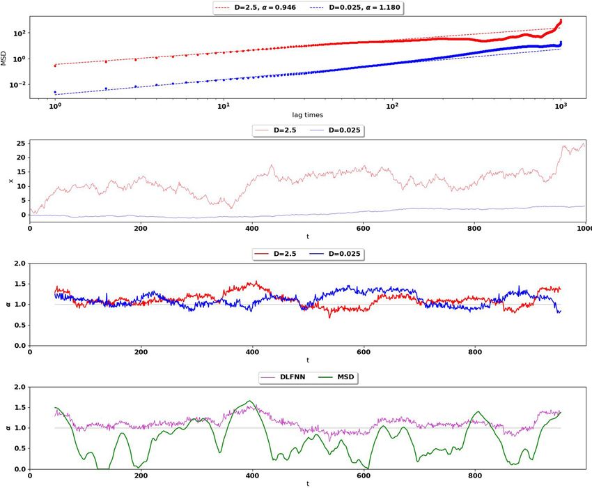
Figure 2. DLFNN analysis of a simulated trajectory. Top: Plot of displacement as a function of time from a simulated fBm trajectory (blue) with multiple
exponent values. Bottom: Hurst exponent values used for simulation (magenta), and the DLFNN exponent predictions of the neural network using a 15
point moving window (black).
(Naslavsky and Caplan, 2018). Many aspects of endosome function are regulated by Rab5, a small
GTPase that is localized to the cytosolic face of early endosomes (Stenmark and Olkkonen, 2001).
Sorting nexin 1 (SNX1) also localises to early endosomes, where it works with the retromer complex
to retrieve and recycle cargoes from early endosomes to the TGN (Simonetti and Cullen, 2019).
SNX1 achieves this through regulating tubular membrane elements on early endosomes by associat-
ing with regions of high membrane curvature (Carlton et al., 2004). Early endosomes mature into
late endosomes, which then fuse with lysosomes, delivering their contents for degradation
(Huotari and Helenius, 2011). Endocytic pathway components are highly dynamic, with microtubule
motors driving long-distance movement while short-range dynamics involve actin-based motility
(Granger et al., 2014; Cabukusta and Neefjes, 2018), making them ideal test cases for DLFNN
analysis. The new method enables the interpretation of experimental trajectories of lysosomes and
endosomes as fBm with stochastic local Hurst exponent, H (t). This in turn allows us to unambigu-
ously and directly classify endosomes and lysosomes to be in anti-persistent or persistent states of
motion at different times. From experiments, we observe that the time spent within these two states
both exhibit truncated heavy-tailed distributions.
To our knowledge, this is the first method which is capable of resolving heterogeneous behavior
of anomalous transport in both time and space. We anticipate that this method will be useful in char-
acterizing a wide range of systems that exhibit anomalous heterogeneous transport. We have there-
fore created a GUI computer application in which the DLFNN is implemented, so that the wider
community can conveniently access this analysis method.
Han et al. eLife 2020;9:e52224. DOI: https://doi.org/10.7554/eLife.52224 4 of 28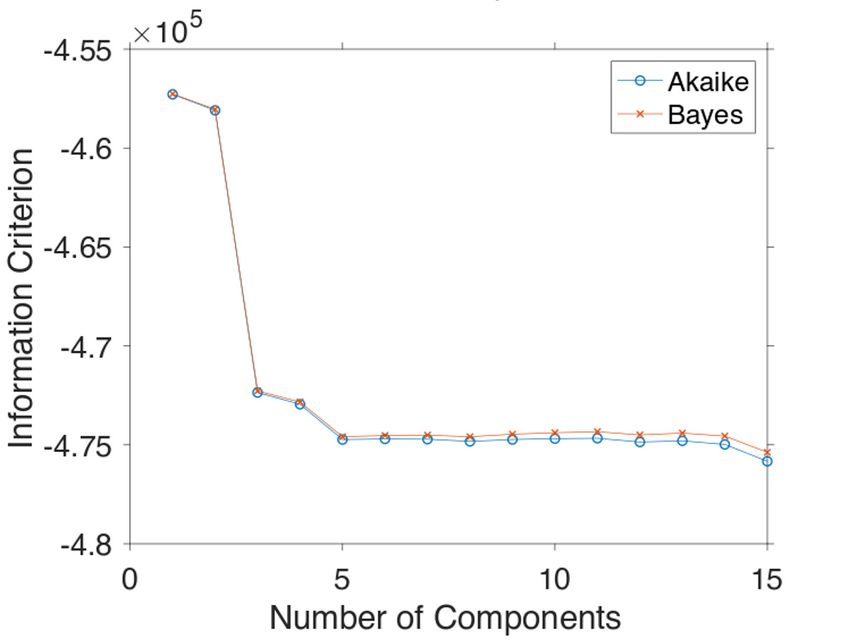
Research article Cell Biology Computational and Systems Biology
Results and discussion
The DLFNN is more accurate than established methods
We tested a DLFNN trained on fBm with three hidden layers of densely connected nodes on
N = 104 computer-generated fBm trajectories each with n = 102 evenly spaced time points and con-
stant Hurst exponent Hsim , randomly chosen between 0 and 1. The DLFNN estimated the Hurst
exponents Hest based on the trajectories, and these were compared with those estimated from
TAMSD, rescaled range, and sequential range methods (Figure 1a). The difference between the sim-
ulated and estimated values DH ¼ Hsim Hest was much smaller for the DLFNN than for the other
methods (Figure 1a), and the DLFNN was ~ 3 times more accurate at estimating Hurst exponents
with a mean absolute error (sH ) ~ 0:05. Also, the errors in estimation of the DLFNN are more stable
across values of Hsim .
Tracking of intracellular motion usually generates trajectories with a variable number of data
points. We therefore compared the performance of the different exponent estimation methods
when the number of evenly spaced, consecutive fBm time points in a trajectory varied over
n ¼ 5; 6; :::; 102 points. The DLFNN maintained an accuracy of sH ~ 0:05 across n, whereas sH of other
methods increase as n decreases (Figure 1b), and was always substantially worse than that of the
DLFNN estimation. Different DLFNN structures (see Figure 1c,d and e) performed similarly, and
introducing more hidden layers did not affect the accuracy of estimation (Figure 1f and g). Given
that the structure of DLFNN does not significantly affect the accuracy of exponent estimation, a tri-
angular densely connected DLFNN was used for all subsequent analyses.
The structure of a triangular DLFNN means that the input layer consists of n nodes, which are
densely connected to n 1 nodes in the first hidden layer, such that at the lth hidden layer, there
would be n l densely connected nodes. Then to estimate the Hurst exponent these nodes are con-
nected to a single node using a Rectified Linear Unit (ReLU) activation function, which returns the
exponent estimate. A triangular DLFNN therefore uses only Ll¼0 ðn lÞ þ 1 nodes for L hidden layers
P
and n input points, whereas the rectangular structure uses nL þ 1 nodes and the anti-triangular struc-
ture uses Ll¼0 ðn þ lÞ þ 1. The triangular structure results in a significant decrease in training parame-
P
ters, and hence computational requirements, while maintaining good levels of accuracy. This
demonstrates that a computationally inexpensive neural network can accurately estimate exponents.
The DLFNN’s estimation capabilities were tested further by inputting nrand randomly sampled
time points from the original fBm trajectories. Surprisingly, sH ~ 0:05 is regained even with just 40
out of 100 data points randomly sampled from the time series for any triangular DLFNN with more
than one hidden layer (Figure 1g). For this method to work with experimental systems, it must esti-
mate Hurst exponents even when the trajectories are noisy. Figure 1h shows how the exponent esti-
mation error increases when Gaussian noise with varying strength compared to the original signal is
added to the fBm trajectories. Importantly, the DLFNN accuracy sH at 20% NSR is as good as the
accuracy of other methods with no noise (compare 1a and h).
To characterize the accuracy of Hsim estimation by the DLFNN, we calculated the bias,
h i
bðHsim Þ ¼ E½Hest Hsim ; variance, VarðHsim Þ ¼ E Hest E½Hest 2 ; and mean square error,
MSE ¼ VarðHsim Þ þ bðHsim Þ2 (Figure 1i). To quantify the efficiency of the estimator the Fisher informa-
tion of the neural network’s estimation needs to be found and the Cramer-Rao lower bound calcu-
lated. The values of bias, variance and MSE were very low (Figure 1i), which taken together with the
simplicity of calculation and the accuracy of estimation even with small number of data points, dem-
onstrates the strength of the DLFNN method. Furthermore, once trained, the model can be saved
and reloaded at any time. Saved DLFNN models, code and the DLFNN Exponent Estimator GUI are
available to download (see Software and Code).
DLFNN allows analysis of simulated trajectories with local stochastic
Hurst exponents
Estimating local Hurst exponents is fundamentally important because much research has focused on
inferring active and passive states of transport within living cells using position-derived quantities
such as windowed MSDs, directionality and velocity (Arcizet et al., 2008; Monnier et al., 2015).
The trajectories are then segmented and Hurst exponents measured in an effort to characterize the
Han et al. eLife 2020;9:e52224. DOI: https://doi.org/10.7554/eLife.52224 5 of 28Research article Cell Biology Computational and Systems Biology
Figure 3. DLFNN analysis of a GFP-Rab5 endosome trajectory. Top: Plot of displacement from a single trajectory in an MRC-5 cell (blue). Shaded areas
show persistent (0.55 < H < 1 in green) and anti-persistent (0 < H < 0.45 in magenta) behaviour. Middle: A 15 point moving window DLFNN exponent
estimate for the trajectory (black) with a line (dashed) marking diffusion H = 0.5 and two lines (dotted) marking confidence bounds for estimation
marking H = 0.45 and 0.55. Bottom: Plot of instantaneous and moving (15 point) window velocity. Right: Plot of the trajectory with start and finish
positions. Persistent (green) and anti-persistent (magenta) segments are shown. For sections that were 0.45 < H < 0.55 were not classified as persistent
or anti-persistent and are depicted in blue.
The online version of this article includes the following figure supplement(s) for figure 3:
Figure supplement 1. DLFNN analysis of a GFP-SNX1-labeled endosome trajectory, depicted as in Figure 3.
Figure supplement 2. DLFNN analysis of a lysosome trajectory, depicted as in Figure 3.
behavior of different cargo when they are actively transported by motor proteins (Chen et al., 2015;
Fedotov et al., 2018) or sub-diffusing in the cytoplasm (Jeon et al., 2011). However, conventional
methods such as the MSD and TAMSD need trajectories with many time points (n ~ 102 103 ) to cal-
culate a single Hurst exponent value with high fidelity. In contrast, the DLFNN enables the Hurst
exponent to be estimated, directly from positional data, for a small number of points. Furthermore,
the DLFNN measures local Hurst exponents without averaging over time points and is able to char-
acterize particle trajectories that may exhibit multi-fractional, heterogeneous dynamics.
To provide a synthetic data set that mimics particle motion in cells, we simulated fBm trajectories
with Hurst exponents that varied in time, and applied a symmetric moving window to estimate the
Hurst exponent using a small number of data points before and after each time point (Figure 2).
The DLFNN was able to identify segments with different exponents, and provided a good running
estimation of the Hurst exponent values. The DLFNN could also handle trajectories with different dif-
fusion coefficients, and generally performed better than MSD analysis when a sliding window was
used (see Appendix B).
DLFNN analysis reveals differences in motile behavior of organelles in
the endocytic pathway
Early endosomes labeled with green fluorescent protein (GFP)-Rab5 undergo bursts of rapid cyto-
plasmic dynein-driven motility interspersed with periods of rest (Flores-Rodriguez et al., 2011;
Zajac et al., 2013). We therefore applied the DLFNN method to experimental trajectories obtained
from automated tracking (Newby et al., 2018) data of GFP-Rab5-labeled endosomes in an MRC-5
cell line that stably expressed GFP-Rab5 at low levels (Figure 3). A moving window of 15 points
identified persistent (green) and anti-persistent (magenta) segments, which corresponded well to
Han et al. eLife 2020;9:e52224. DOI: https://doi.org/10.7554/eLife.52224 6 of 28Research article Cell Biology Computational and Systems Biology
the moving window velocity plots (Figure 3, lower panel), confirming that the neural network is
indeed distinguishing passive states from active transport states with non-zero average velocity. We
then used it to analyze the motility of two other endocytic compartments: SNX1-positive endosomes
(Allison et al., 2017; Hunt et al., 2013) and lysosomes (Cabukusta and Neefjes, 2018;
Hendricks et al., 2010). It successfully segmented tracks of GFP-SNX1 endosomes (Figure 3—fig-
ure supplement 1) in a stable MRC-5 cell line (Allison et al., 2017) and lysosomes visualized using
lysobrite dye (Figure 3—figure supplement 2). A total of 63–71 MRC-5 cells were analyzed, giving
40,800 (GFP-Rab5 endosome), 11,273 (GFP-SNX1 endosome) and 38,039 (lysosome) tracks that
were segmented into 277,926 (GFP-Rab5), 215,087 (GFP-SNX1) and 474,473 (lysosome) persistent
or anti-persistent sections, each yielding a displacement, duration and average H.
These data revealed intriguing similarities and differences in behavior between the three endo-
cytic components. Analysis of the duration and displacement of segments (Appendix C) revealed
that all organelles spent longer in anti-persistent than persistent states (Figure 4) but moved much
further when persistent (Appendix 3—figure 1), as expected. However, GFP-SNX1 endosomes
spent much less time than GFP-Rab5 endosomes or lysosomes in an anti-persistent state (Figure 4).
This difference in behavior was also seen when histograms of the Hurst exponents were plotted (Fig-
ure 5), as SNX1 endosomes were much less likely to exhibit anti-persistent behavior, particularly with
H0.5mm from their start point were selected, which yielded 2369
Rab5, 2099 SNX1 and 7645 lysosome persistent segments that were then analyzed to give the dura-
tion, displacement and velocity of anterograde and retrograde excursions (Figure 7; Table 1). The
anti-persistent segments contained within these tracks were also analyzed.
These statistics revealed that each endocytic organelle moved with different characteristics. GFP-
Rab5 endosomes moved much faster than GFP-SNX1 endosomes or lysosomes, particularly in the
retrograde direction (Figure 7, upper panel). Strikingly, although the GFP-SNX1 endosomes were
slowest in both directions, they moved furthest and for longest in each segment, in keeping with the
longer duration of persistent segments seen in the global analysis of tracks (Figure 4) and higher H
values (Figure 5). The differences in behavior between Rab5 and SNX1 endosomes is intriguing,
since both are recruited to the early endosome by the lipid phosphoinositol-3-phosphate
(Christoforidis et al., 1999; Carlton et al., 2004; Behnia and Munro, 2005; Huotari and Helenius,
2011). However, SNX1 also senses membrane curvature (Carlton et al., 2004), and immunofluores-
cence labeling of MRC-5 cells with antibodies to Rab5 and SNX1 demonstrated that they reside on
distinct domains of larger early endosomes (Figure 6—figure supplement 1), as expected
van Weering et al. (2012). In addition, while SNX1 endosomes were usually Rab5-positive, there
Han et al. eLife 2020;9:e52224. DOI: https://doi.org/10.7554/eLife.52224 7 of 28Research article Cell Biology Computational and Systems Biology
Rab5
0
10
Anti-persistent
Persistent
Power law:
Power law:
-5
10
-1 0 1
10 10 10
SNX1
0
10
Anti-persistent
Persistent
Power law:
Power law:
10 -5
10 -1 10 0 10 1
Lyso
0
10
Anti-persistent
Persistent
Power law:
Power law:
10 -5
10 -1 10 0 10 1
Figure 4. Survival functions plotted with error bars for persistent and anti-persistent segments for Rab5-positive endosomes, SNX1-positive endosomes
and lysosomes with the power-law fits. Fit parameters can be found in Appendix 3—table 1.
Han et al. eLife 2020;9:e52224. DOI: https://doi.org/10.7554/eLife.52224 8 of 28Research article Cell Biology Computational and Systems Biology
b8 Rab5
Exp. Data
GMM fit
6 Component I
Component II
P(H)
4 Component III
Component IV
Component V
a 2 Component VI
7
Rab5 0
0 0.2 0.4 0.6 0.8 1
6 SNX1
Lyso c8 SNX1
5 Exp. Data
GMM fit
6 Component I
4
P(H)
Component II
P(H)
4 Component III
Component IV
3 Component V
2 Component VI
2 0
0 0.2 0.4 0.6 0.8 1
1
d8 Lyso
Exp. Data
0 GMM fit
0 0.2 0.4 0.6 0.8 1 6 Component I
H Component II
P(H)
4 Component III
Component IV
Component V
2 Component VI
0
0 0.2 0.4 0.6 0.8 1
H
Figure 5. Comparison of Hurst exponent distributions for GFP-Rab5, GFP-SNX1 and lysosomes. (a) Histograms of Hurst exponents for GFP-Rab5
(black), GFP-SNX1 (magenta) endosomes and lysosomes (green) plot on the same axes for comparison. The individual histograms of Hurst exponents
(black solid) for GFP-Rab5-tagged endosomes, GFP-SNX1-tagged endosomes and lysosomes are shown in (b, c and d) respectively. For each
histogram, the Gaussian mixture model fit for six components (red dashed) and individual Gaussian distribution components are shown on the same
plot. The number of components were chosen through the Bayes information criterion shown in Appendix 4—figure 1.
was a significant population of Rab5 endosomes that lacked SNX1, especially smaller early endo-
somes that were often located in the cell periphery. It is likely that this population of Rab5-positive,
SNX1-negative endosomes is particularly motile. The high retrograde velocity of these endosomes
might be explained by the recruitment of dynein to Rab5 endosomes via Hook family members
(Bielska et al., 2014; Zhang et al., 2014; Schroeder and Vale, 2016; Guo et al., 2016). These
dynein adaptors have the intriguing property of recruiting two dyneins per dynactin
(Urnavicius et al., 2018; Grotjahn et al., 2018), leading to faster rates of movement in motility
assays using purified protein than adaptors that only recruit one dynein per dynactin. Perhaps, SNX1
endosomes move more slowly than Rab5 endosomes because they use a ‘single-dynein’ adaptor. An
alternative explanation could be that SNX1 endosomes are slowed down by interactions with the
actin cytoskeleton, since SNX1 domains are enriched in the WASH complex, which in turn controls
localized actin assembly (Gomez and Billadeau, 2009; Simonetti and Cullen, 2019). Actin might
also contribute to the slow, steady motion of SNX1 endosomes via myosin motors or the formation
of actin comets (Simonetti and Cullen, 2019). These interesting possibilities remain to be tested
experimentally.
The analysis of anterograde and retrograde segments revealed that lysosomes moved at moder-
ate speed, and were equally fast in both directions, but each burst of movement was short (Figure 7,
upper panels). In addition, pauses were 4 times longer for lysosomes than either early endosome
type (Figure 7, lower panels). Lysosomes also often changed direction of movement (e.g. Figure 3—
figure supplement 2), as previously reported (Hendricks et al., 2010). So far, no activating dynein
adaptor has been identified on lysosomes (Reck-Peterson et al., 2018), although several potential
Han et al. eLife 2020;9:e52224. DOI: https://doi.org/10.7554/eLife.52224 9 of 28Research article Cell Biology Computational and Systems Biology
Figure 6. MRC-5 cells stably expressing GFP-Rab5, GFP-SNX1 or stained with Lysobrite with tracking data overlaid. The colours show the value of H
estimated by the neural network using a 15 point window. The scalebar is 10 mm.
The online version of this article includes the following video and figure supplement(s) for figure 6:
Figure supplement 1. Distribution of endogenous Rab5 and SNX1.
Figure 6—video 1. Video of MRC-5 cell stably expressing GFP-Rab5.
https://elifesciences.org/articles/52224#fig6video1
Figure 6—video 2. Video of MRC-5 cell stably expressing GFP-SNX1.
https://elifesciences.org/articles/52224#fig6video2
Figure 6—video 3. Video of MRC-5 cell stained with Lysobrite.
https://elifesciences.org/articles/52224#fig6video3
dynein interactors have been identified, such as RILP (Rab7 interacting lysosomal protein
(Cabukusta and Neefjes, 2018). Whether this underlies the difference in motile behavior between
lysosomes and early endosomes remains to be tested: however, a less active dynein could well con-
tribute to frequent reversals in direction (Hancock, 2014).
fBm with a stochastic Hurst exponent is a new possible intracellular
transport model
fBm is a Gaussian process BH ðtÞ with zero mean and covariance hBH ðtÞBH ðsÞi ~ t2H þ s2H ðt sÞ2H ,
where the Hurst exponent, H is a constant between 0 and 1. With the DLFNN providing local esti-
mates of the Hurst exponent, the motion of endosomes and lysosomes can be described as fBm
with a stochastic Hurst exponent, HðtÞ. This is different to multifractional Brownian motion
(Peltier and Lévy Véhel, 1995) where HðtÞ is a function of time. In our case, HðtÞ is itself a stochastic
process and such a process has been considered theoretically (Ayache and Taqqu, 2005). This is the
first application of such a theory to intracellular transport and opens a new method for characterizing
vesicular movement. Furthermore, Figure 3 shows that the motion of a vesicle, BH ðtÞ, exhibits
regime switching behavior between persistent and anti-persistent states.
We found that the times that lysosomes and endosomes spend in a persistent and anti-persistent
state are heavy-tailed (Figure 4). These times are characterized by the probability densities
ðtÞ ~ t 1 , where anti-persistent states have 0 < m < 1 and persistent states have 1 < m < 2. Exten-
sive plots and fittings are shown in Figure 4 and Appendix C. In fact, the residence time probability
density has an infinite mean to remain in an anti-persistent state (0Research article Cell Biology Computational and Systems Biology Figure 7. Box and whisker plots of displacements, times and velocities of persistent retrograde, persistent anterograde and anti-persistent segments in experimental trajectories. Any segment with H>0:55 was classed as persistent and H
Research article                                                               Cell Biology Computational and Systems Biology

                                      Materials and methods
Key resources table
Reagent type or resource Designation                 Source                 Identifiers                      Additional information
Cell line                     Lung fibroblast line   Allison et al., 2017   GFP-SNX1-MRC5                    MRC5 cell line stably expressing
(Homo sapiens)                                       https://doi.org/                                        GFP-SNX1. Mycoplasma free.
                                                     10.1083/
                                                     jcb.201609033
Cell line                     Lung fibroblast line   Other                  GFP-Rab5-MRC5                    MRC5 cell line stably expressing
(H. sapiens)                                                                                                 GFP-Rab5 generated by retroviral
                                                                                                             transduction by G. Pearson and
                                                                                                             E. Reid, University of Cambridge.
                                                                                                             Mycoplasma free.
Cell line                     MRC-5 SV1 TG1          ECACC                  MRC-5 SV1 TG1 cells,             Mycoplasma free.
(H. sapiens)                  Lung fibroblast line                          cat no. 85042501
Antibody                      Anti-human Rab5A       Cell Signalling        3547S                            IF(1/200)
                              Rabbit monoclonal      Technology
Antibody                      Anti-human sorting     BD Biosciences         611482                           IF(1/200)
                              nexin 1
                              (mouse monoclonal)
Antibody                      Alexa594-conjugated    Jackson                715-585-150                      IF(1/400)
                              anti-mouse IgG         ImmunoResearch
                              (donkey polyclonal)
Antibody                      A488-conjugated donkey Jackson                711-545-152                      IF(1/400)
                              anti-rabbit IgG        Immunoresearch
Recombinant                   pLXIN-GFP-             Other                                                   Used by G. Pearson and
DNA reagent                   Rab5C-I-NeoR                                                                   E. Reid, University of Cambridge
                                                                                                             to generate retrovirus
                                                                                                             containing GFP-Rab5C
Sequence-                     Hpa1 GFP Forward       Other                  PCR primer                       Used by G. Pearson and
based reagent                                                                                                E. Reid, University of Cambridge
                                                                                                             to generate retrovirus
                                                                                                             containing GFP-Rab5C.
                                                                                                             TAGGGAGTTAACATGGTGAG
                                                                                                             CAAGGGCGAGGA
Sequence-                     Not1 Rab5C Reverse     Other                  PCR primer                       Used by G. Pearson and
based reagent                                                                                                E. Reid, University of
                                                                                                             Cambridge to generate
                                                                                                             retrovirus containing
                                                                                                             GFP-Rab5C .
                                                                                                             ATCCCTGCGGCCGCTCAGTT
                                                                                                             GCTGCAGCACTGGC
Chemical                      DAPI                   Biolegend              422801                           IF (1 mg/mL)
compound, drug
Chemical                      Prolong Gold           ThermoFisher           P36930
compound, drug
Chemical                      Lysobrite Red          AAT Bioquest           22645                            (1/2500)
compound, drug
Chemical                      Geneticin (G418)       Sigma-Aldrich          G1397                            200 mg/mL to maintain
compound, drug                                                                                               GFP-Rab5-MRC5 and
                                                                                                             GFP-SNX1-MRC5 cells
                                                                                                             in culture.
Chemical                      Formaldehyde           Sigma-Aldrich          252549
compound, drug                solution, 37% (wt/v)
Chemical                      Triton X-100           Anatrace               T1001
compound, drug
Software, algorithm           NNT (aitracker.net)    Newby et al., 2018     AITracker                        Web-based automated
                                                                                                             tracking service
Software, algorithm           Metamorph              Molecular              Metamorph                        Metamorph Microscopy
                                                     Devices LLC                                             Automation and Image
                                                                                                             Analysis Software
Continued on next page

Han et al. eLife 2020;9:e52224. DOI: https://doi.org/10.7554/eLife.52224                                                         12 of 28
Research article Cell Biology Computational and Systems Biology
Continued
Reagent type or resource Designation Source Identifiers Additional information
Software, algorithm FIJI Schindelin, J.; Arganda- FIJI/ImageJ
Carreras,
I. and Frise, E. et al. (2012) ,
‘Fiji: an open-source
platform for biological-
image analysis’, Nature
methods 9 (7): 676–682,
PMID22743772,
DOI: 10.1038/nmeth.2019
Software, algorithm DLFNN Exponent Han, Daniel. (2020, DLFNN/DLFNN Exponent Estimator Hurst exponent estimator with
Estimator January 20). Deep Learning Feed-forward
DLFNN Exponent Neural Network application for
Estimator (Version 0). Windows 10. Documentation
http://doi.org/ included.
10.1101/777615
Software, algorithm Python3 Python Software Python/Python3
Foundation.Python
Language Reference 3.7.
Available at
www.python.org
Software, algorithm SciPy Virtanen et al. (2020) SciPy/scipy
SciPy 1.0: Fundamental
Algorithms for Scientific
Computing in Python.
Nature Methods,
in press.
Software, algorithm Tensorflow Abadi et al., 2016 Tensorflow
Software, algorithm Keras Chollet, François and Keras
others. ‘Keras.’ (2015).
Available from
https://keras.io
Software, algorithm fbm Flynn, Christopher, FBM package in Python Exact methods for simulating
fbm 0.3.0 available fractional Brownian motion
for download at (fBm) or fractional Gaussian
https://pypi.org/ noise (fGn) in python.
project/fbm/ Approximate simulation of
or multifractional Brownian motion
https://github.com/ (mBm) or multifractional
crflynn/fbm Gaussian noise (mGn).
Other 35 mm glass- Ibidi Cat. No. 81150
bottomed dishes
(m-Dish)
Hurst exponent estimation methods
Time averaged MSDs were calculated using
N n
1 X
hx2 ðndtÞi ¼ ½xððm þ nÞdt Þ xðmdtÞ2 (1)
N n m¼0
where xðndtÞ is the track displacement at time ndt and a track contains N coordinates spaced at regu-
lar time intervals of dt. From now on, hxi will denote the time average of x unless explicitly specified
otherwise. The total time is T ¼ ðN 1Þdt and n ¼ 1; 2; :::; N 1. Lag-times are the set of possible ndt
within the data set and hx2 ðndtÞi was then fit to a power-law ~ t 2H using the ‘scipy.optimize’ package
in Python3 to estimate the exponent H.
Rescaled ranges were calculated by creating a mean adjusted cumulative deviate series
zðndtÞ ¼ nm¼0 xðmdtÞ hxi from original displacements xðndtÞ and mean displacement hxi. Then the
P
rescaled range is calculated by
max fzgn min fzgn
½R=SðndtÞ ¼ qffiffiffiffiffiffiffiffiffiffiffiffiffiffiffiffiffiffiffiffiffiffiffiffiffiffiffiffiffiffiffiffiffiffiffiffiffiffiffiffiffiffiffiffiffiffiffiffiffiffiffiffiffiffiffiffiffi (2)
hxðndtÞiÞ2
1
Pn
ndt m¼0 ð xðmdtÞ
Han et al. eLife 2020;9:e52224. DOI: https://doi.org/10.7554/eLife.52224 13 of 28Research article Cell Biology Computational and Systems Biology
Table 1. Statistics of experimental trajectory segments.
The persistent and anti-persistent segments in this table are: from trajectories that travelled over 0.5 mm at any point from their initial
starting positions; contained more points than the window size; and switched behavior more than twice in the trajectory. Note that
these conditions are much stricter than those to generate Figures 4 and 5. Each persistent segment was then further subdivided into
retrograde and anterograde segments (see Materials and methods).
Rab5 SNX1 Lyso
Number of persistent segments 2369 2099 7645
Number of anti-persistent segments 6983 3947 19,320
Number of retrograde segments 2925 2343 5882
Number of anterograde segments 2303 1609 6827
Anti-persistent displacement (mm) Mean 0.05 0.05 0.03
Median 0.04 0.05 0.03
St. Dev 0.02 0.01 0.004
Anti-persistent speed (mms-1) Mean 0.82 0.75 0.10
Median 0.70 0.73 0.09
St. Dev 0.31 0.19 0.02
Anti-persistent time (s) Mean 0.23 0.20 0.93
Median 0.23 0.19 0.92
St. Dev 0.05 0.03 0.11
Retrograde displacement (mm) Mean 0.53 0.74 0.29
Median 0.49 0.69 0.29
St. Dev 0.19 0.28 0.08
Retrograde speed (mms-1) Mean 2.29 1.35 1.49
Median 2.21 1.29 1.46
St. Dev 0.87 0.39 0.25
Retrograde time (s) Mean 0.22 0.46 0.17
Median 0.21 0.45 0.17
St. Dev 0.09 0.09 0.03
Anterograde displacement (mm) Mean 0.35 0.43 0.31
Median 0.33 0.37 0.32
St. Dev 0.17 0.20 0.08
Anterograde speed (mms-1) Mean 2.06 1.10 1.51
Median 1.71 1.08 1.48
St. Dev 0.95 0.30 0.27
Anterograde time (s) Mean 0.18 0.34 0.18
Median 0.15 0.33 0.18
St. Dev 0.08 0.08 0.03
where fzgn ¼ zð0Þ; zðdtÞ; zð2dtÞ; :::; zðndtÞ. The rescaled range is then fitted to a power law
½R=SðndtÞ ~ ðndtÞH where H is the Hurst (1951). The ‘compute_Hc’ function in the ‘hurst’ package in
Python3 estimates the Hurst exponent in this way.
Sequential ranges are defined as
MðndtÞ ¼ sup ðxðsÞ xð0ÞÞ inf ðxðsÞ xð0ÞÞ (3)
0sndt 0sndt
where supðxÞ is the supremum and infðxÞ is the infimum for the set x of real numbers. Then
MðndtÞ ¼ ðndtÞH MðdtÞ Feller (1951).
Han et al. eLife 2020;9:e52224. DOI: https://doi.org/10.7554/eLife.52224 14 of 28Research article Cell Biology Computational and Systems Biology
DLFNN structure and training
The fractional Brownian trajectories were generated using the Hosking method within the ‘FBM’
function available from the ‘fbm’ package in Python3. The DLFNN was built using Tensorflow
Abadi et al. (2016) and Keras Chollet (2015) in Python3 and trained by using the simulated frac-
tional Brownian trajectories. The training and testing of the neural network were performed on a
workstation PC equipped with 2 CPUs with 32 cores (Intel(R) Xeon CPU E5-2640 v3) and 1 GPU (NVI-
DIA Tesla V100 with 16 GB memory). The structure of the neural network was a multilayer, feedfor-
ward neural network where all nodes of the previous layer were densely connected to nodes of the
next layer. Each node had a ReLU activation function and the parameters were optimized using the
RMSprop optimizer (see Keras documentation Chollet, 2015). Three separate structures were
explored and examples of these structures for two hidden layers and five time point inputs are
shown in Figure 1g,h and i. The triangular structure was predominantly used since this was the least
computationally expensive and accuracy between different structures were similar. To compare the
accuracy of different methods, the mean absolute error (sH ) of N trajectories,
sH ¼ Nm¼1 Hnsim Hnest =N, was used. Before inputting values into the neural network, the time series
P
was differenced to make it stationary. The input values of a fBm trajectory f xg ¼ x0 ; x1 ; :::; xn were dif-
ferenced and normalized so that
xinput ¼ ðx1 x0 Þ=rangeðxÞ; ðx2 x1 Þ=rangeðxÞ; :::; ðxn xn 1 Þ=rangeðxÞ. Since the model requires dif-
ferenced and normalized input values, in theory it should be applicable to a wide range of datasets.
However, further testing must be done in order to confirm this expectation.
Gaussian kernel density estimation
Kernel density estimation (KDE) is a non-parametric method to estimate the probability density func-
tion (PDF) of random variables. If N random variables xn are distributed by an unknown density func-
tion PðxÞ, then the kernel density estimate PðxÞ is
N
^ ¼1
x x
n
X
PðxÞ K (4)
N n¼1 l
where KðÞ is the kernel function and l is the bandwidth. In this paper, we have used a Gaussian
2
KDE, KðyÞ ¼ p1ffiffiffiffi
2p
e y =2 , to estimate the two dimensional PDFs of the second and bottom row in
Figure 1a. This was performed in Python3 using ‘scipy.stats.gaussian_kde’ and Scott’s rule of thumb
for bandwidth selection.
Segmenting trajectories into persistent and anti-persistent segments
From the estimates of Hurst exponent from the DLFNN, trajectories were segmented into persistent
and anti-persistent segments. Given an experimental trajectory x ¼ x0 ; x1 ; :::; xn and window of length
Nw (an odd number) starting at xi , we obtain the H estimate for the position at xj , where
j ¼ i þ ðNw 1Þ=2. This will give us a series of Ht values, HðNw 1Þ=2 ; HðNw 1Þ=2þ1 ; :::; Hn ðNw 1Þ=2 , which cor-
respond to the positions, xðNw 1Þ=2 ; xðNw 1Þ=2þ1 ; :::; xn ðNw 1Þ=2 . Then, the values Ht can be segmented
into consecutive points of persistence Ht >0:55 and anti-persistence HtResearch article Cell Biology Computational and Systems Biology
from the centrosome to the current particle position xi and the vector, ~
ri;iþ1 , from the current particle
position to the next particle position xiþ1 . The exact formula is cosðÞ ¼ ~ r0;i ~ ri;iþ1 j. Using
r0;i jj~
ri;iþ1 =j~
windows in a similar fashion as determining persistent and anti-persistent segments, cosði Þ corre-
sponding to position xi was found for the points within a persistent segment. If cosði Þ>scosðÞ , then
the motion was deemed to be anterograde and if cosði Þ< scosðÞ , retrograde. Sweeping through
the points of xi , consecutive retrograde or anterograde points formed segments from the persistent
segments. A threshold of scosðÞ ¼ 0:3 was used.
Cell lines
The MRC-5 SV1 TG1 Lung fibroblast cell line was purchased from ECACC. MRC-5 cell lines stably
expressing GFP-Rab5C and GFP-SNX1 were kindly provided by Drs. Guy Pearson and Evan Reid
(Cambridge Institute for Medical Research, University of Cambridge). The GFP-SNX1 cell line has
been previously described in Allison et al. (2017). Cell lines were routinely tested for mycoplasma
infection. To generate the MRC-5 GFP-Rab5C stable cell line, GFP-Rab5C was PCRed from pIRES
GFP-Rab5C Seaman (2004) using ‘Hpa1 GFP Forward’ (TAGGGAGTTAACATGGTGAGCAAGGGC-
GAGGA) and ‘Not1 Rab5C Reverse’ (ATCCCTGCGGCCGCTCAGTTGCTGCAGCACTGGC) oligonu-
cleotide primers. The GFP-Rab5C PCR product and a pLXIN-I-NeoR plasmid were digested using
Hpa1 (New England Biolabs - R0105) and Not1 (New England Biolabs - R3189) restriction enzymes.
The GFP-Rab5C PCR product was then ligated into the digested pLXIN-I-NeoR using T4 DNA Ligase
(New England Biolabs - M0202). The ligated plasmid was amplified in bacteria selected with ampicil-
lin and verified using Sanger Sequencing. To generate the GFP-Rab5C MRC-5 cell line, Phoenix ret-
rovirus producer HEK293T cells were transfected with the pLXIN-GFP-Rab5C-I-NeoR plasmid to
generate retrovirus containing GFP-Rab5C. MRC-5 cells were inoculated with the virus, and success-
fully transduced cells were selected using 200 mg/mL Geneticin (G418 - Sigma-Aldrich G1397). Cells
used for imaging were not clonally selected.
Live-imaging and tracking
Stably expressing MRC-5 cells were co-stained with LysoBrite Red (AAT Bioquest), imaged live using
fluorescence microscopy and tracked with NNT aitracker.net; Newby et al. (2018). The cells were
grown in MEM (Sigma Life Science) and 10% FBS (HyClone) and incubated for 48 hr at 37 in 5% CO2
on 35 mm glass-bottomed dishes (m-Dish, Ibidi, Cat. No. 81150). For LysoBrite staining, LysoBrite
was diluted 1 in 500 with Hank’s Balanced Salt solution (Sigma Life Science). Then 0.5 mL of this solu-
tion was added to cells on a 35 mm dish containing 2 mL of growing media and incubated at 37 for
at least 1 hr. Cells were then washed with sterile PBS and the media replaced with growing media.
After at least 6 hr incubation, the growing media was replaced with live-imaging media com-
posed of Hank’s Balanced Salt solution (Sigma Life Science, Cat. No. H8264) with added essential
and non-essential amino acids, glutamine, penicillin/streptomycin, 25 mM HEPES (pH 7.0) and 10%
FBS (HyClone). Live-cell imaging was performed on an inverted Olympus IX71 microscope with an
Olympus 100 1.35 oil PH3 objective. Samples were illuminated using an OptoLED (Cairn Research)
light source with 470 nm and white LEDs. For GFP, a 470 nm LED and Chroma ET470/40 excitation
filter was used in combination with a Semrock FITC-3540C filter set. For Lysobrite-Red, a white light
LED, Chroma ET573/35 was used with a dualband GFP/mCherry dichroic and an mCherry emission
filter (ET632/60). GFP-Rab5-labeled endosomes were imaged in a total of 65 cells, from three inde-
pendent experiments. GFP-SNX1-labeled endosomes were imaged in a total of 63 cells from four
independent experiments. Lysosomes were imaged in separate experiments, with 71 cells imaged
from three independent repeats. A stream of 20 ms exposures was collected with a Prime 95B
sCMOS Camera (Photometrics) for 17 s using Metamorph software while the cells were kept at 37
(in atmospheric CO2 levels). The endosomes and lysosomes in the videos were then tracked using
an automated tracking software (AITracker) Newby et al. (2018).
Confocal imaging
To compare the localization of SNX1 and Rab5, GFP-Rab5-MRC-5 cells were grown on #1.5 cover-
slips and then fixed in 3% (w/v) formaldehyde in PBS for 20 min at room temperature (RT). Coverslips
were washed twice in PBS, quenched in PBS with glycine, then permeabilized by incubation for
5 min in 0.1% Triton X-100. After another wash in PBS, coverslips were labeled with antibodies to
Han et al. eLife 2020;9:e52224. DOI: https://doi.org/10.7554/eLife.52224 16 of 28Research article Cell Biology Computational and Systems Biology
SNX1 and Rab5 for 1 h at RT, washed three times in PBS, then labeled with Alexa488-donkey anti-
rabbit and Alexa594-donkey anti-mouse antibodies in 1 mg/mL DAPI in PBS for 30 min. After three
PBS washes, coverslips were dipped in deionized water, air-dried and mounted on slides using Pro-
long Gold.
Images were collected on a Leica TCS SP8 AOBS inverted confocal using a 100x/1.40 NA PL apo
objective. The confocal settings were as follows: pinhole, one airy unit; scan speed 400 Hz unidirec-
tional; format 2048 2048. Images were collected using hybrid detectors (A488 and A594) or a
PMT (DAPI) with these detection mirror settings; [Alexa488, 498 nm-577 nm; Alexa594, 602 nm-
667 nm; DAPI, 420 nm-466 nm] using the SuperK Extreme supercontinuum white light laser for
488 nm (10.5%) and 594 nm (5%) excitation, and a 405 nm laser (5%) for DAPI. Images were col-
lected sequentially to eliminate cross-talk between channels. When acquiring 3D optical stacks the
confocal software was used to determine the optimal number of Z sections. The data were decon-
volved using Huygens software before generating maximum intensity projections of 3D stacks using
FIJI.
Software and code
The code and documentation for determining the Hurst exponent can be found in https://github.
com/dadanhan/hurst-exp (copy archived at https://github.com/elifesciences-publications/hurst-
exp; Han, 2019) and a GUI is available on https://zenodo.org/record/3613843#.XkPf2Wj7SUl.
Acknowledgements
The authors thank: Dr. Jay Newby and Zach Richardson (UNC Chapel Hill) for assistance in using the
automated tracking system (AITracker); Prof. Philip Woodman, Prof. Martin Lowe, Prof. Matthias
Weiss (Universität Bayreuth), Dr. Henry Cox, Dr. Jack Hart, Rebecca Yarwood and Hannah Perkins
for discussions; and, Dr. Guy Pearson and Dr. Evan Reid (University of Cambridge) for providing the
GFP-Rab5 and GFP-SNX1 MRC-5 cell lines. DH acknowledges financial support from the Wellcome
Trust Grant No. 215189/Z/19/Z. SF, NK, TAW, and VJA acknowledge financial support from EPSRC
Grant No. EP/J019526/1. VJA acknowledges support from the Biotechnology and Biological Scien-
ces Research Council grant number BB/H017828/1. AG acknowledges financial support from the
Wellcome Trust Grant No. 108867/Z/15/Z. The Leica SP8 microscope used in this study was pur-
chased by the University of Manchester Strategic Fund. Special thanks goes to Dr. Peter March for
his help with the confocal imaging.
Additional information
Funding
Funder Grant reference number Author
Wellcome Trust 215189/Z/19/Z Daniel Han
EPSRC EP/J019526/1 Nickolay Korabel
Victoria J Allan
Sergei Fedotov
Thomas A Waigh
BBSRC BB/H017828/1 Victoria J Allan
Wellcome Trust 108867/Z/15/Z Anna Gavrilova
The funders had no role in study design, data collection and interpretation, or the
decision to submit the work for publication.
Author contributions
Daniel Han, Conceptualization, Data curation, Software, Formal analysis, Validation, Investigation,
Visualization, Methodology, Writing - original draft, Project administration, Writing - review and edit-
ing; Nickolay Korabel, Formal analysis, Validation, Investigation, Writing - review and editing; Runze
Chen, Software, Formal analysis; Mark Johnston, Validation, Investigation; Anna Gavrilova, Data
Han et al. eLife 2020;9:e52224. DOI: https://doi.org/10.7554/eLife.52224 17 of 28Research article Cell Biology Computational and Systems Biology
curation, Investigation; Victoria J Allan, Conceptualization, Resources, Data curation, Formal analysis,
Supervision, Funding acquisition, Validation, Investigation, Visualization, Methodology, Project
administration, Writing - review and editing; Sergei Fedotov, Conceptualization, Resources, Formal
analysis, Supervision, Funding acquisition, Validation, Methodology, Project administration, Writing -
review and editing; Thomas A Waigh, Conceptualization, Supervision, Validation, Methodology,
Project administration, Writing - review and editing
Author ORCIDs
Daniel Han https://orcid.org/0000-0002-9088-1651
Victoria J Allan https://orcid.org/0000-0003-4583-0836
Thomas A Waigh https://orcid.org/0000-0002-7084-559X
Decision letter and Author response
Decision letter https://doi.org/10.7554/eLife.52224.sa1
Author response https://doi.org/10.7554/eLife.52224.sa2
Additional files
Supplementary files
. Transparent reporting form
Data availability
Supporting files are on GitHub and Zenodo.
The following dataset was generated:
Database and
Author(s) Year Dataset title Dataset URL Identifier
Daniel Han 2020 DLFNN Exponent Estimator https://zenodo.org/re- Zenodo, 3613843#.
cord/3613843#. XmzM0pP7RRY
XmzM0pP7RRY
References
Abadi M, Barham P, Chen J, Chen Z, Davis A, Dean J, Devin M, Ghemawat S, Irving G, Isard M. 2016.
Tensorflow: a system for large-scale machine learning. 12th USENIX Symposium on Operating Systems Design
and Implementation.
Allison R, Edgar JR, Pearson G, Rizo T, Newton T, Günther S, Berner F, Hague J, Connell JW, Winkler J,
Lippincott-Schwartz J, Beetz C, Winner B, Reid E. 2017. Defects in ER-endosome contacts impact lysosome
function in hereditary spastic paraplegia. Journal of Cell Biology 216:1337–1355. DOI: https://doi.org/10.1083/
jcb.201609033, PMID: 28389476
Amblard F, Maggs AC, Yurke B, Pargellis A, Leibler S. 1996. Subdiffusion and anomalous local viscoelasticity in
actin networks. Physical Review Letters 77:4470–4473. DOI: https://doi.org/10.1103/PhysRevLett.77.4470,
PMID: 10062546
Arcizet D, Meier B, Sackmann E, Rädler JO, Heinrich D. 2008. Temporal analysis of active and passive transport
in living cells. Physical Review Letters 101:248103. DOI: https://doi.org/10.1103/PhysRevLett.101.248103,
PMID: 19113674
Ariel G, Rabani A, Benisty S, Partridge JD, Harshey RM, Be’er A. 2015. Swarming Bacteria migrate by lévy walk.
Nature Communications 6:1–6. DOI: https://doi.org/10.1038/ncomms9396
Ayache A, Taqqu MS. 2005. Multifractional processes with random exponent. Publicacions Matemàtiques 49:
459–486. DOI: https://doi.org/10.5565/PUBLMAT_49205_11
Ba Q, Raghavan G, Kiselyov K, Yang G. 2018. Whole-Cell scale dynamic organization of lysosomes revealed by
spatial statistical analysis. Cell Reports 23:3591–3606. DOI: https://doi.org/10.1016/j.celrep.2018.05.079,
PMID: 29925001
Bálint Š, Verdeny Vilanova I, Sandoval Álvarez Á, Lakadamyali M. 2013. Correlative live-cell and superresolution
microscopy reveals cargo transport dynamics at Microtubule intersections. PNAS 110:3375–3380. DOI: https://
doi.org/10.1073/pnas.1219206110, PMID: 23401534
Banks DS, Fradin C. 2005. Anomalous diffusion of proteins due to molecular crowding. Biophysical Journal 89:
2960–2971. DOI: https://doi.org/10.1529/biophysj.104.051078, PMID: 16113107
Barabási AL. 2005. The origin of bursts and heavy tails in human dynamics. Nature 435:207–211. DOI: https://
doi.org/10.1038/nature03459, PMID: 15889093
Han et al. eLife 2020;9:e52224. DOI: https://doi.org/10.7554/eLife.52224 18 of 28Research article Cell Biology Computational and Systems Biology
Barkai E, Garini Y, Metzler R. 2012. Strange kinetics of single molecules in living cells. Physics Today 65:29–35.
DOI: https://doi.org/10.1063/PT.3.1677
Behnia R, Munro S. 2005. Organelle identity and the signposts for membrane traffic. Nature 438:597–604.
DOI: https://doi.org/10.1038/nature04397, PMID: 16319879
Bielska E, Schuster M, Roger Y, Berepiki A, Soanes DM, Talbot NJ, Steinberg G. 2014. Hook is an adapter that
coordinates kinesin-3 and dynein cargo attachment on early endosomes. The Journal of Cell Biology 204:989–
1007. DOI: https://doi.org/10.1083/jcb.201309022, PMID: 24637326
Bondarenko AN, Bugueva TV, Dedok VA. 2016. Inverse problems of anomalous diffusion theory: An artificial
neural network approach. Journal of Applied and Industrial Mathematics 10:311–321. DOI: https://doi.org/10.
1134/S1990478916030017
Bressloff PC, Newby JM. 2013. Stochastic models of intracellular transport. Reviews of Modern Physics 85:135–
196. DOI: https://doi.org/10.1103/RevModPhys.85.135
Cabukusta B, Neefjes J. 2018. Mechanisms of lysosomal positioning and movement. Traffic 19:761–769.
DOI: https://doi.org/10.1111/tra.12587
Carlton J, Bujny M, Peter BJ, Oorschot VM, Rutherford A, Mellor H, Klumperman J, McMahon HT, Cullen PJ.
2004. Sorting nexin-1 mediates tubular endosome-to-TGN transport through coincidence sensing of high-
curvature membranes and 3-phosphoinositides. Current Biology 14:1791–1800. DOI: https://doi.org/10.1016/j.
cub.2004.09.077, PMID: 15498486
Chen K, Wang B, Granick S. 2015. Memoryless self-reinforcing directionality in endosomal active transport within
living cells. Nature Materials 14:589–593. DOI: https://doi.org/10.1038/nmat4239, PMID: 25822692
Chenouard N, Smal I, de Chaumont F, Maška M, Sbalzarini IF, Gong Y, Cardinale J, Carthel C, Coraluppi S,
Winter M, Cohen AR, Godinez WJ, Rohr K, Kalaidzidis Y, Liang L, Duncan J, Shen H, Xu Y, Magnusson KE,
Jaldén J, et al. 2014. Objective comparison of particle tracking methods. Nature Methods 11:281–289.
DOI: https://doi.org/10.1038/nmeth.2808, PMID: 24441936
Chollet F. 2015. keras. GitHub. https://github.com/fchollet/keras
Christoforidis S, Miaczynska M, Ashman K, Wilm M, Zhao L, Yip SC, Waterfield MD, Backer JM, Zerial M. 1999.
Phosphatidylinositol-3-OH kinases are Rab5 effectors. Nature Cell Biology 1:249–252. DOI: https://doi.org/10.
1038/12075, PMID: 10559924
Deng Y, Bao F, Dai Q, Wu LF, Altschuler SJ. 2019. Scalable analysis of cell-type composition from single-cell
transcriptomics using deep recurrent learning. Nature Methods 16:311–314. DOI: https://doi.org/10.1038/
s41592-019-0353-7, PMID: 30886411
Ernst D, Hellmann M, Köhler J, Weiss M. 2012. Fractional brownian motion in crowded fluids. Soft Matter 8:
4886–4889. DOI: https://doi.org/10.1039/c2sm25220a
Evans R, Jumper J, Kirkpatrick J, Sifre L, Green T, Qin C, Zidek A, Nelson A, Bridgland A, Penedones H. 2018.
De novo structure prediction with deeplearning based scoring. Annual Review of Biochemistry 77:6.
Fedotov S, Korabel N, Waigh TA, Han D, Allan VJ. 2018. Memory effects and lévy walk dynamics in intracellular
transport of cargoes. Physical Review E 98:042136. DOI: https://doi.org/10.1103/PhysRevE.98.042136
Feller W. 1951. The asymptotic distribution of the range of sums of independent random variables. The Annals
of Mathematical Statistics 22:427–432. DOI: https://doi.org/10.1214/aoms/1177729589
Flores-Rodriguez N, Rogers SS, Kenwright DA, Waigh TA, Woodman PG, Allan VJ. 2011. Roles of dynein and
dynactin in early endosome dynamics revealed using automated tracking and global analysis. PLOS ONE 6:
e24479. DOI: https://doi.org/10.1371/journal.pone.0024479, PMID: 21915335
Fuliński A. 2017. Fractional brownian motions: memory, diffusion velocity, and correlation functions. Journal of
Physics A: Mathematical and Theoretical 50:054002. DOI: https://doi.org/10.1088/1751-8121/50/5/054002
Getz WM, Saltz D. 2008. A framework for generating and analyzing movement paths on ecological landscapes.
PNAS 105:19066–19071. DOI: https://doi.org/10.1073/pnas.0801732105, PMID: 19060192
Gomez TS, Billadeau DD. 2009. A FAM21-containing WASH complex regulates retromer-dependent sorting.
Developmental Cell 17:699–711. DOI: https://doi.org/10.1016/j.devcel.2009.09.009, PMID: 19922874
Granger E, McNee G, Allan V, Woodman P. 2014. The role of the cytoskeleton and molecular motors in
endosomal dynamics. Seminars in Cell & Developmental Biology 31:20–29. DOI: https://doi.org/10.1016/j.
semcdb.2014.04.011, PMID: 24727350
Grotjahn DA, Chowdhury S, Xu Y, McKenney RJ, Schroer TA, Lander GC. 2018. Cryo-electron tomography
reveals that dynactin recruits a team of dyneins for processive motility. Nature Structural & Molecular Biology
25:203–207. DOI: https://doi.org/10.1038/s41594-018-0027-7, PMID: 29416113
Guo X, Farı́as GG, Mattera R, Bonifacino JS. 2016. Rab5 and its effector FHF contribute to neuronal polarity
through dynein-dependent retrieval of somatodendritic proteins from the axon. PNAS 113:E5318–E5327.
DOI: https://doi.org/10.1073/pnas.1601844113, PMID: 27559088
Han D. 2019. hurst-exp. GitHub. 9. https://github.com/dadanhan/hurst-exp
Hancock WO. 2014. Bidirectional cargo transport: moving beyond tug of war. Nature Reviews Molecular Cell
Biology 15:615–628. DOI: https://doi.org/10.1038/nrm3853, PMID: 25118718
Harrison AW, Kenwright DA, Waigh TA, Woodman PG, Allan VJ. 2013. Modes of correlated angular motion in
live cells across three distinct time scales. Physical Biology 10:036002. DOI: https://doi.org/10.1088/1478-3975/
10/3/036002, PMID: 23574726
Hendricks AG, Perlson E, Ross JL, Schroeder HW, Tokito M, Holzbaur EL. 2010. Motor coordination via a tug-of-
war mechanism drives bidirectional vesicle transport. Current Biology 20:697–702. DOI: https://doi.org/10.
1016/j.cub.2010.02.058, PMID: 20399099
Han et al. eLife 2020;9:e52224. DOI: https://doi.org/10.7554/eLife.52224 19 of 28You can also read