Statistical approaches for identification of low-flow drivers: temporal aspects - HESS
←
→
Page content transcription
If your browser does not render page correctly, please read the page content below
Hydrol. Earth Syst. Sci., 23, 447–463, 2019
https://doi.org/10.5194/hess-23-447-2019
© Author(s) 2019. This work is distributed under
the Creative Commons Attribution 4.0 License.

Statistical approaches for identification of low-flow drivers:
temporal aspects
Anne Fangmann and Uwe Haberlandt
Institute of Hydrology and Water Resources Management, Leibniz University of Hannover, Germany

Correspondence: Anne Fangmann (fangmann@iww.uni-hannover.de)

Received: 24 May 2018 – Discussion started: 19 June 2018
Revised: 17 December 2018 – Accepted: 18 December 2018 – Published: 25 January 2019

Abstract. The characteristics of low-flow periods, especially     including Mosley (2000), who analyzed the influence of El
regarding their low temporal dynamics, suggest that the di-       Niño and La Niña effects on monthly lowest 7-day flow in
mensions of the metrics related to these periods may be eas-      New Zealand. He determined a major deviation of low flows
ily related to their meteorological drivers using simplified      from the normal in La Niña years. Haslinger et al. (2014)
statistical model approaches. In this study, linear statistical   found that correlations between streamflow anomalies and
models based on multiple linear regressions (MLRs) are pro-       meteorological drought indices are high, especially within
posed. The study area chosen is the German federal state of       the low-flow period. Van Loon and Laaha (2015) analyzed
Lower Saxony with 28 available gauges used for analysis. A        the dependence of streamflow drought duration and deficit
number of regression approaches are evaluated. An approach        volume on climatic indicators and catchment descriptors,
using principal components of local meteorological indices        while Liu et al. (2015) estimated the parameters of a GEV
as input appeared to show the best performance. In a second       distribution fitted to the low-flow time series at their gauge in
analysis it was assessed whether the formulated models may        China as functions of a set of climatic indices.
be eligible for application in climate change impact analysis.       Based on these findings it is hypothesized that stream-
The models were therefore applied to a climate model en-          flow metrics describing low-flow events may be efficiently
semble based on the RCP8.5 scenario. Analyses in the base-        assessed based on their relationship with metrics of meteo-
line period revealed that some of the meteorological indices      rological states. This assumption entails that simple statis-
needed for model input could not be fully reproduced by the       tical models may be formulated that allow a reproduction of
climate models. The predictions for the future show an over-      low-flow metrics based on meteorological input. In this study
all increase in the lowest average 7-day flow (NM7Q), pro-        the relationship between annual low flow and a variety of
jected by the majority of ensemble members and for the ma-        meteorological indices will be analyzed with the aim of for-
jority of stations.                                               mulating simple statistical models. Such models will be set
                                                                  up individually for each catchment in the study area and are
                                                                  supposed to be capable of predicting low flow as a simple
                                                                  function of several relevant meteorological indices in time.
1   Introduction                                                  Various temporal scales will be considered for the meteoro-
                                                                  logical data and the most adequate ones for each catchment
Low flows appear ideal for the analysis of statistical depen-     will be identified. The model fitting itself will be carried out
dencies with their meteorological drivers, due to their spe-      using various statistical approaches in order to account for
cific characteristics. As opposed to high flows, low stream-      different effects, like non-stationarity or serial dependence
flow is usually far less dynamic, and its meteorological          in the annual low-flow indices. In order to assess the perfor-
drivers, i.e., primarily a lack of rain and increased evapora-    mance of the strictly linear statistical approaches, they will
tion, are observable over much larger scales in both time and     be compared to a hydrological model, which is assumed to
space. Accordingly, several studies have aimed at explaining      accurately reproduce rainfall–runoff relationships by involv-
observed peculiarities in low flows by climatic phenomena,

Published by Copernicus Publications on behalf of the European Geosciences Union.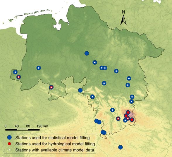
448                         A. Fangmann and U. Haberlandt: Statistical approaches for identification of low-flow drivers

ing more complex processes, relying on continuous meteo-
rological input. This analysis will reveal whether the statisti-
cal models fail to acknowledge important nonlinear relation-
ships.
   Apart from identifying relevant low-flow drivers, we test
whether the use of the formulated statistical models may be
extended to prediction of future low flows, using meteorolog-
ical input from climate models. The probably most common
approach in hydrological climate change impact analysis is
to drive hydrological models, usually rainfall–runoff models
of variable complexity, with regional climate model data in-
put, obtained for various emission scenarios. Also for low
flows this model chain has been applied for impact assess-
ment in several studies, e.g., by de Wit et al. (2007), Schnei-
der et al. (2013), Forzieri et al. (2014), Wanders and Van La-
nen (2015), van Vliet et al. (2015), Roudier et al. (2016),
or Gosling et al. (2017). The statistical models may pose an
alternative simpler impact model approach that is easily set
up and applied to large numbers of catchments and exten-
sive climate model ensembles – while predicting hydrologi-         Figure 1. Study area with stations available for different analyses.
cal quantities with sufficient accuracy. They may thus offer a
different yet convenient tool for comprehensive regional cli-
mate change impact analyses. According to this hypothesis,         mate data, i.e., available records from 1951 to 2010. After
the formulated models will be applied to an ensemble of re-        removal of heavily influenced gauges, 28 stations remain for
gional climate model data in order to assess the plausibility      analysis, as depicted in Fig. 1. Catchment sizes range from
of their low-flow projections in the future.                       24 to 37 720 km2 . In previous work (NLWKN, 2017), a hy-
                                                                   drological model was set up for seven of these stations, as
2     Study area and data                                          indicated in Fig. 1. This selection of stations will be used for
                                                                   comparing statistical and hydrological model performance.
2.1    Study area
                                                                   2.3   Indices
The area under investigation is the federal state of Lower
Saxony situated in northwestern Germany. Its total area of         The daily time series of meteorological and streamflow data
47 634 km2 extends from the North Sea in the northwest to          are used to compute indices, which form the basis for all
the Harz mountains in the southeast. The largest portion of        models. Target variables are a variety of annual low-flow in-
Lower Saxony is part of the North German Plain, where              dices. They are selected in a way to represent different quan-
the terrain is generally flat and low. The highest elevations      tities of interest for low-flow analysis (e.g., intensity, dura-
are found in the secondary mountains of the Harz, at up to         tion, and timing). The low-flow indices used in this study
971 m a.s.l. The topography is depicted in Fig. 1.                 are shown in Table 1. In order to exclude winter low flows,
                                                                   which may be subject to different underlying processes, the
2.2    Base data                                                   indices are computed for the summer half-year (May to Oc-
                                                                   tober) only. Within the region most low-flow events occur
The meteorological data used in this work comprise daily           between June and October.
time series of precipitation, temperature, and global radia-           The selected low-flow indices represent a small fraction of
tion. The data are made available continuously in space via        possible indices but cover quite a range of low-flow quan-
interpolation onto a 1×1 km raster for the total area of Lower     tities relevant for water resource management and planning.
Saxony. Regionalization is based on 771 precipitation gauges       Non-exceedance quantiles represent the overall low-flow sit-
and 123 climatic stations and carried out for the period from      uation in a year without specific relation to a certain event.
1951 to 2010. The regionalization process is described in de-      The same holds for average volume and duration. NMxQ,
tail in NLWKN (2012).                                              maximum volume and duration, as well as timing, on the
   Daily time series are also used for streamflow. In total,       other hand, focus on the greatest events per year in their re-
there are 353 flow records of average daily discharge avail-       spective terms and characterize them accordingly. The con-
able in and around the study area. Record lengths range from       sideration of variations within the individual index types
7 to 193 years. For analysis in this work, gauges have been        (e.g., Q95 and Q80 ) is not solely owing to different man-
selected that have a maximum overlap with the available cli-       agement requirements but is used to investigate the various

Hydrol. Earth Syst. Sci., 23, 447–463, 2019                                        www.hydrol-earth-syst-sci.net/23/447/2019/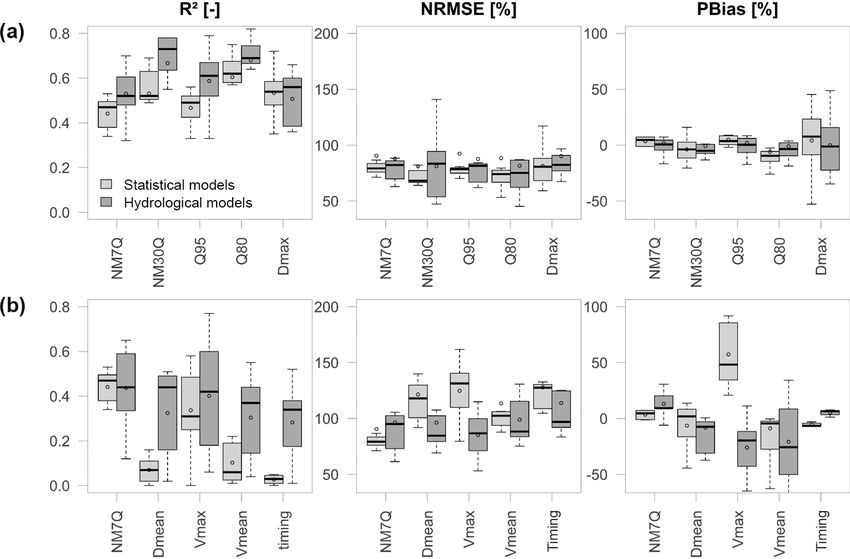
A. Fangmann and U. Haberlandt: Statistical approaches for identification of low-flow drivers                                           449

Table 1. List of low-flow indices.

            Index       Unit         Description
            Q95
                        m3 s−1       5 % and 20 % non-exceedance quantiles of the daily average discharge
            Q80
            NM7Q
                        m3 s−1       Lowest 7- and 30-day average flow
            NM30Q
            Vmax                     Maximum and mean deficit volume: sum of daily discharge below the long-term 20 %
                        m3
            Vmean                    non-exceedance quantile
            Dmax                     Maximum and mean low-flow duration: number of days with discharge below the long-term
                        d
            Dmean                    20 % non-exceedance quantile
            timing      –            Day of the year on which smallest daily flow occurs

models’ capability to reproduce both more and less extreme               3     Methods
low flows.
   Meteorological indices are used as input for the models.              The aim is to model a desired low-flow index on an annual
Like for their low-flow counterparts, annual values are calcu-           basis as a function of a combination of meteorological in-
lated from daily time series of precipitation sums, mean and             dices observed in time. Several methods will be analyzed
maximum temperature, and global radiation, averaged over                 for this purpose in order to identify the one most suitable
the respective basins of the considered discharge gauges. Ta-            for modeling the relationships in consideration of their later
ble 2 summarizes the applied indices and gives a short de-               application for far-future predictions. These methods are de-
scription.                                                               scribed in the following.
   While the low-flow indices are calculated for a fixed pe-
riod within the year (the summer half-year), the period for              3.1    Multiple linear regression
computation of the meteorological quantities is varied in
                                                                         Multiple linear regression (MLR) is probably the most com-
length and position. Figure 2 shows the schema according to
                                                                         mon method to model relationships between variables and
which every meteorological index has been computed. INQ
                                                                         will pose the basis for several methods in this work. It aims
represents the low-flow index, calculated for its fixed period
                                                                         at reproducing a target variable y as a linear combination of k
within a given year. IM denotes the meteorological index.
                                                                         explanatory variables x1 , . . . xk . The general shape of a mul-
The first number in the index notation represents the length
                                                                         tiple linear regression model is the following:
of the base period for calculation (e.g., 3, 6, or 12 months),
while the second one indicates the lead time, i.e., the num-             y = β0 + β1 x1 + . . . + βk xk + ε.                            (1)
ber of months the period is shifted back in time relative to
the low-flow index. A 0-shift indicates that the calculation             The regression coefficients β1 , . . . βk are estimated in two dif-
period ends simultaneously with the low-flow period.                     ferent ways, i.e., (a) an ordinary least squares (OLS) proce-
                                                                         dure and (b) a generalized least squares (GLS) fitting. The
2.4   Climate model data                                                 latter method involves the inclusion of the covariance matrix
                                                                         of the residuals, which allows for correction for both het-
An ensemble of 15 coupled global and regional climate                    eroscedasticity and dependence of the residuals. Since het-
models is applied for climate change impact analysis. An                 eroscedasticity did not appear to be a relevant issue in this
overview is shown in Table 3. The datasets are based on                  study, while serial correlation in the data did, autoregressive
simulations of global climate models of CMIP5 run on an                  (AR) covariance structures of various orders are tested to de-
RCP8.5 scenario. The data are available on a 10×10 km grid.              scribe the residual covariance. The elements of an AR(1) co-
   The climate model data have been pre-processed in pre-                variance structure, for example, can be described via
vious work (NLWKN, 2017) and are available for a smaller
domain than the observed climate data. Therefore, basin av-              σij = σ 2 ρ |i−j | ,                                           (2)
erages can only be computed for 17 of the 28 stations, as
                                                                         where ρ denotes the autocorrelation between terms with lag
shown in Fig. 1.
                                                                         1.
                                                                            The need for and order of the considered AR process is de-
                                                                         termined using the likelihood ratio test on a case-by-case ba-
                                                                         sis. This parametric test is developed to test the superiority of
                                                                         more complex models over their simpler forms, i.e., whether

www.hydrol-earth-syst-sci.net/23/447/2019/                                                  Hydrol. Earth Syst. Sci., 23, 447–463, 2019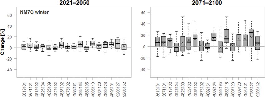
450                             A. Fangmann and U. Haberlandt: Statistical approaches for identification of low-flow drivers

Figure 2. Calculation scheme for low-flow indices with a fixed base period and meteorological indices with a varying base period and lead
times relative to the low-flow calculation period.

Table 2. Meteorological indices based on precipitation, temperature, and potential evapotranspiration.

            Index           Unit        Description
            Pmean           mm d−1      Average daily precipitation
            Px              mm d−1      Non-exceedance quantiles of daily precipitation sums
                                        Standardized Precipitation Index: standardized deviation of accumulated precipitation
            SPI             –
                                        sums from the long-term normal (Mckee et al., 1993)
            DSDmean
                            d           Mean and maximum dry spell duration: number of days with preciptation < 1 mm d−1
            DSDmax
            WSDmean
                            d           Mean and maximum wet spell duration: number of days with preciptation ≥ 1 mm d−1
            WSDmax
            Tmin
            Tmean           ◦C          Minimum, mean, and maximum daily average temperature
            Tmax
                                        Heat wave duration: number of days above 90 % non-exceedance quantile of maximum
            HWD             d
                                        temperature calculated for each specific day of the year
            ETPmean         mm d−1      Average daily potential evaporation calculated according to Turc–Wendling
            P -ETPmean      mm d−1      Average climatic water balance: precipitation minus potential evapotranspiration
            P / ETPmean     –           Aridity index: ratio of average precipitation and potential evapotranspiration
                                        Standardized Precipitation Evaporation Index: standardized deviation of accumulated
            SPEI            –
                                        climatic water balance from the long-term normal (Vicente-Serrano et al., 2010)

a model with a higher number of parameters performs sig-                 planatory variables in a model arises. As such, for a small
nificantly better than the same model with fewer parameters.             data set, only a small number of uncorrelated regressors
Performance is thereby measured in terms of maximized log-               should be selected. At the same time however, leaving out
likelihood function values and the (1−α) quantile of the Chi2            important explanatory variables may drastically lower the
distribution, whose degrees of freedom are chosen as the dif-            predictive power of the model. In order to overcome the re-
ference in the number of parameters between the compared                 strictions given through the limited period of observation,
models (Coles, 2001).                                                    a principal component analysis (PCA) is applied, merging
                                                                         many explanatory variables into a few uncorrelated compo-
3.2   Principal component analysis                                       nents that pose the ideal basis for model fitting on limited
                                                                         data with maximum exploitation of information. PCA is car-
The fitting of multiple linear regression models is restricted           ried out by firstly centering the set of p explanatory vari-
by sample size. Fitting a model with a large number of re-               ables X∗ via subtraction of their respective means. Then, the
gressors to a small data set will result in over-fitting. Ad-            (p × p) covariance matrix 6 is computed and its eigenval-
ditionally, the problem of multicollinearity between the ex-             ues λ1 , λ2 , . . . λp and eigenvectors γ 1 , γ 2 , . . . , γ p are deter-

Hydrol. Earth Syst. Sci., 23, 447–463, 2019                                               www.hydrol-earth-syst-sci.net/23/447/2019/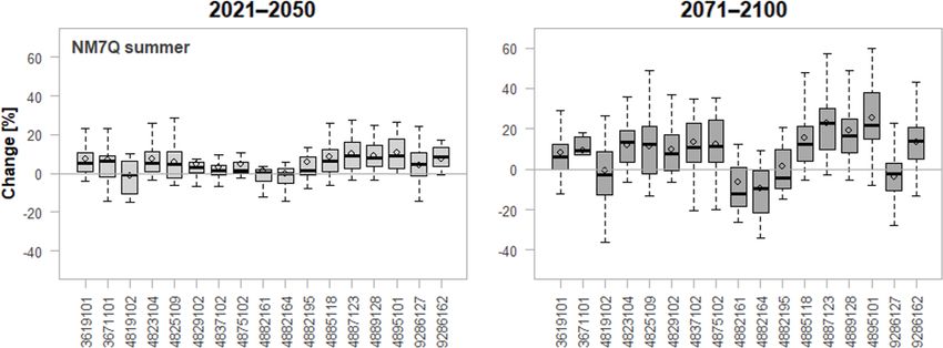
A. Fangmann and U. Haberlandt: Statistical approaches for identification of low-flow drivers                                        451

Table 3. List of coupled global and regional climate models used for analysis.

                      Global model                             Regional model                Short name
                                                               CLMcom-CCLM4-8-17             CNRM-CCLM
                      CNRM-CERFACS-CNRM-CM5 run1
                                                               SMHI-RCA4                     CNRM-RCA4
                      ICHEC-EC-EARTH run12                     CLMcom-CCLM4-8-17             EC-EARTH-CCLM
                      ICHEC-EC-EARTH run3                      DMI-HIRHAM5                   EC-EARTH-HIRHAM5
                      ICHEC-EC-EARTH run1                      KNMI-RACMO22E                 EC-EARTH-RACMO22E
                      ICHEC-EC-EARTH run12                     SMHI-RCA4                     EC-EARTH-RCA4
                                                               CLMcom-CCLM4-8-17             HadGEM2-CCLM
                      MOHC-HadGEM2-ES run1                     RACMO22E                      HadGEM2-RACMO22E
                                                               SMHI-RCA4                     HadGEM2-RCA4
                      IPSL-INERIS-CM5A-MR run1                 SMHI-RCA4                     IPSL-RCA4
                      IPSL-CM5A-MR                             WRF331F                       IPSL-WRF331F
                                                               CLMcom-CCLM4-8-17             MPI-ESM-CCLM
                                                               SMHI-RCA4                     MPI-ESM-RCA4
                      MPI-M-MPI-ESM-LR run1
                                                               REMO2009 run1                 MPI-ESM-REMO1
                                                               REMO2009 run2                 MPI-ESM-REMO2

mined. Multiplication of the eigenvectors with X ∗ yields the           3.4      Model fitting and evaluation
following system of equations:
                                                                        Given the vast number of meteorological indices, variable
                                                                        selection for the statistical models becomes paramount. In
 y1 = γ 11 x1 + γ 21 x2 + . . . + γ p1 xp                               order to select appropriate indices and restrict the num-
 y2 = γ 12 x1 + γ 22 x2 + . . . + γ p2 xp                               bers of selected regressors, a two-way stepwise approach
                    ..                    ,                     (3)     for variable selection is chosen that aims at minimizing the
                     .                                                  Bayesian information criterion (BIC; Schwarz, 1978) of the
 yp = γ 1p x1 + γ 2p x2 + . . . + γ pp xp                               final model. The BIC is closely related to the Aikaike infor-
                                                                        mation criterion (AIC; Aikaike, 1974) but penalizes variable
                                                                        inclusion stricter for larger sample sizes, which is the reason
where y1 , y2 , . . . , yp denote the principal components, sorted      for its selection in this study. The smaller the BIC, the better
according to their contribution to the total variance of data at        the predictive power of a model. The algorithm for variable
hand. The eigenvectors represent the respective loading of a            selection randomly selects a variable and adds variables to
variable x on a principal component y.                                  the model that decrease the overall BIC. After each addition
                                                                        it is tested whether the removal of any of the existing vari-
3.3   Hydrological modeling                                             ables in the model leads to further decrease in the BIC.
                                                                           Since the number of potential regressors in this study is
                                                                        high and variables may be strongly related, a second criterion
In order to evaluate the performance of the statistical ap-             is included in the BIC-minimization procedure. In order to
proaches, hydrological modeling is applied as the bench-                prevent multicollinearity, the variance inflation factor (VIF)
mark for prognosis of future flow. The rainfall–runoff model            of each variable added to the model is computed. The VIF
used here is an adaptation of the Swedish HBV by Lind-                  is a measure of how much of the variance of a predictor in a
strom et al. (1997), denoted HBV-IWW. The specifics of the              model can be explained by the other predictors in the same
model are described in detail, e.g., in Wallner et al. (2013).          model. Computation is done via
A schematic overview of the structure of the model is pre-
sented in Fig. 3. The model is semi-distributed and can be                           1
applied on the sub-catchment scale. Input is daily precip-              VIF =            ,                                          (4)
                                                                                  1 − R2
itation, temperature, and potential evapotranspiration. The
model comprises five routines and a variety of parameters               where R 2 denotes the coefficient of determination of a re-
controlling the translation between the various model com-              gression model that describes the variable to be added as a
ponents. The parameters are automatically optimized using               function of the existing variables in the model. The recom-
the AMALGAM evolutionary multimethod algorithm (Vrugt                   mended limits for the VIF vary throughout literature. Since
and Robinson, 2007).                                                    multicollinearity is a major issue for the analyses of this

www.hydrol-earth-syst-sci.net/23/447/2019/                                               Hydrol. Earth Syst. Sci., 23, 447–463, 2019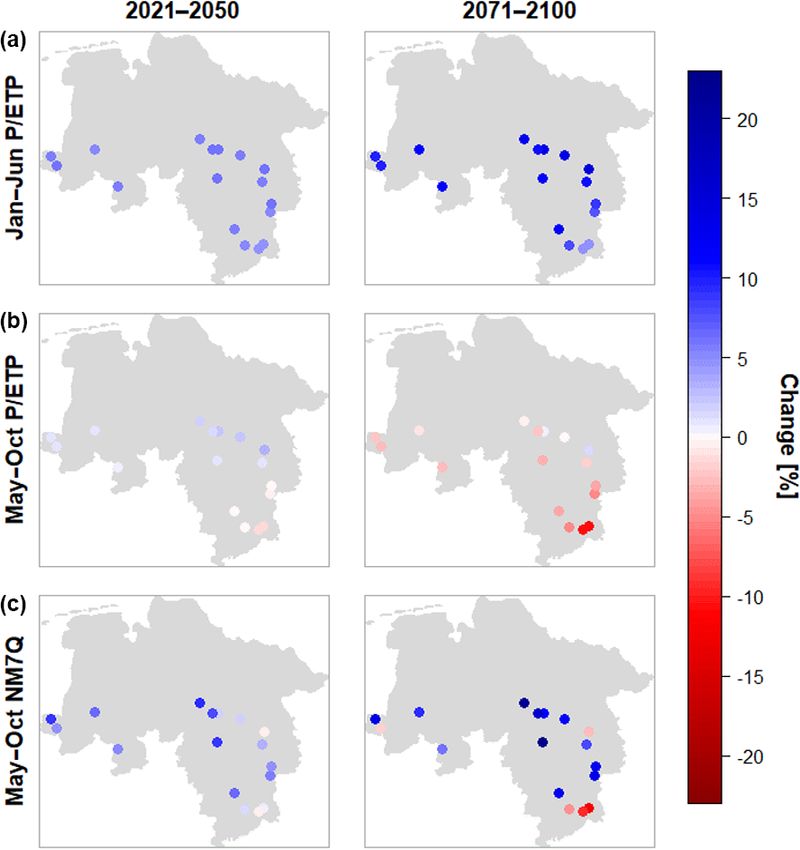
452                          A. Fangmann and U. Haberlandt: Statistical approaches for identification of low-flow drivers

Figure 3. Vertical structure of the HBW-IWW model according to Wallner et al. (2013).

study, a low value of 5 has been chosen. Variables that show          to the former validation period and evaluated in the calibra-
higher VIFs are not included into the existing model.                 tion period. The inversion is applied in order to preserve the
   For the GLS models with AR-correlation structure, vari-            continuity of the time series.
able selection was carried out according to OLS model fit-               In order to compare the quality of the different model
ting, evaluating the necessity of the AR-structure for each           approaches, a selection of performance measures is com-
added variable using the likelihood ratio test. For variable          puted. These measures include the coefficient of determina-
selection using principal components, the BIC-minimization            tion (R 2 ), the normalized root mean square error (NRMSE),
strategy is extended, not by adding each additional variable          and the percent bias (pbias). The criteria are selected to show
directly to the model but by computing principal components           various aspects of model quality, i.e., information about the
first and testing them as potential regressors of the model.          similarity of the course of simulated and observed time se-
   In contrast to the statistical models, the hydrological            ries, the average fit, and systematic errors.
model is based on daily input and output and is therefore
capable of modeling an entire year’s hydrograph rather than           3.5   Climate change impact analysis
a single low-flow metric. Calibrating the hydrological model
on the complete hydrograph may reduce the predictability of           The most suitable statistical model is eventually applied us-
the single low-flow event and favor the statistical models (di-       ing the ensemble of climate model data. The first step is the
rectly calibrated on the low-flow value) in a comparison of           assessment of the performance of the model chains in re-
model performances. Therefore, the HBV-IWW is calibrated              producing the observed low flow. This analysis is done in
in a strategy comparable to the statistical approaches, namely        a reference period from 1971 to 2000. The projections and
by including nothing but the desired annual low-flow metric           changes in the low flow will be analyzed in near- (2021–
in the objective function.                                            2050) and far-future (2071–2100) periods. It should be noted
   In order to allow for a proper assessment of the models’ ca-       that the aim of the prognosis using actual climate model data
pabilities of predicting future low flows, the available record       is primarily for the validation of the statistical model ap-
at each station is split equally into a calibration and a vali-       proaches rather than a detailed regional assessment of ex-
dation period. Both periods are continuous in time and the            pected changes.
calibration consistently precedes the validation period. This            In order to account for potential bias in the climate model
setup is chosen to test the ability of models fitted to a past        data used for prediction of future low flow, the individual
period of time to predict “future”, i.e., the validation period’s     station models are recalibrated for each climate model sepa-
characteristics. In order to double the available periods for         rately. The problem that needs to be overcome for this pro-
validation, the time series are inversed and models are fitted        cess is the matching of the temporarily dissociated series of
                                                                      meteorological indices generated by the climate models with

Hydrol. Earth Syst. Sci., 23, 447–463, 2019                                             www.hydrol-earth-syst-sci.net/23/447/2019/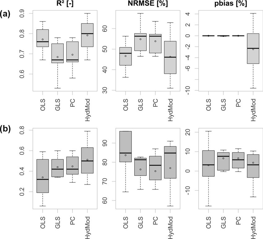
A. Fangmann and U. Haberlandt: Statistical approaches for identification of low-flow drivers                                      453

                                                                      dian value of 0.58. The PC model also shows the smallest
                                                                      percent bias with a median of 1.30 %. The inclusion of sev-
                                                                      eral variables in the form of principal components appears
                                                                      meaningful in order to avoid omittance of important regres-
                                                                      sors and potential multicollinearity, granted by the orthogo-
                                                                      nality of the components. Additionally, the principal compo-
                                                                      nent models are supposedly more robust against outliers in
                                                                      single variables.
                                                                         The second best performance is shown by the GLS-fitted
                                                                      model with an AR-correlation structure. One should note that
                                                                      an AR-correlation structure has not been used for model fit-
                                                                      ting at every station. Only at those stations where the likeli-
                                                                      hood ratio test favored an inclusion was a GLS fitting carried
                                                                      out. This was the case for 55 % of the fitted models (35 %
                                                                      AR(1) covariance structure, 20 % AR(2) covariance struc-
                                                                      ture). The bias in the calibration period arises through the
                                                                      approximation of the unknown true autocorrelation structure
                                                                      in the data. Since the values are negligibly small, this approx-
Figure 4. Performance criteria of different model approaches in the   imation is considered reasonable. As the number of variables
calibration period (a) and validation period (b) over 28 stations.    included in the GLS model is significantly lower compared to
                                                                      the principal component model, and the step of finding suit-
                                                                      able components was skipped, the performance based on the
the observed low-flow time series, which is handled as fol-           close validation period, as shown here, appears to be compa-
lows. At first, the explanatory variables identified in the ob-       rably good. However, inclusion of AR processes via likeli-
served model fitting procedure are carried over; i.e., no new         hood ratio testing results in some distortion of the residuals
variable selections are carried out. This is meaningful, since        and violation of the prerequisites of linear regression fitting
the selected variables represent observed low-flow drivers.           at several stations. Thus, the principal component model is
The principal components are then re-estimated for the se-            considered favorable.
lected variables as projected by the individual climate mod-             Figure 5 shows the same criteria as Fig. 4 with inclusion of
els. In order to relate the climate model data to the observed        the hydrological model, and thus for a total of seven stations
time series, the regression parameters are optimized in such a        only. The performance of the HBV model in both calibration
way that the empirical distribution of the predicted low flow         and validation periods is substantially better in all aspects,
matches that of the observed sample. In order for the recali-         with a median validation R 2 of 0.50, an NRMSE of 76.1 %,
brated model to be no more precise than the originally fitted         and a percent bias of 1.7 %, compared to the PC model with
model, which may lead to false estimates of the regression            median values of 0.42 %, 78.4 %, and 5.8 %, respectively.
coefficients, the model fitted to the observed data is used as        This performance however could only be achieved using
the target during re-calibration rather than the observed low-        the calibration strategy of matching exclusively the annual
flow series itself.                                                   NM7Q values at each station. Calibration using the entire
                                                                      hydrograph or parts of the flow duration curve did not ex-
4     Results and discussion                                          plicitly outperform the statistical approaches. Nevertheless,
                                                                      HBV-IWW appears to be suitable for assessment of future
4.1    Model performance                                              low-flow development when calibrated specifically on low-
                                                                      flow indices.
Performance of the individual MLR model variants are com-                The statistical models appear to be positively biased. At
pared using the aforementioned performance measures. Fig-             almost all investigated stations a positive mean error could
ure 4 shows the model performance of all tested model con-            be observed. As models are fitted in both directions to the
figurations exemplary for NM7Q prediction in the calibra-             time series, this error appears to originate in the model it-
tion (top) and validation period (bottom). For the validation         self, rather than in underlying processes of the time series
period one can clearly observe an increase in performance             that cannot be captured. Overall differences in model per-
from left to right, i.e., an increasing predictive power with         formance between the stations could not be correlated with
increasing model complexity. The OLS-fitted model shows               any specific regions or catchment features. The quality of the
poorest performance with a median R 2 of only 0.43.                   simulation did not depend on catchment size, position in the
   The highest predictive performance has been achieved               study area, or any other distinguishable factor.
with the principal component model. The coefficient of de-               An obvious problem is the significant difference in model
termination for the MLR model over all stations has a me-             performance between the calibration and validation periods.

www.hydrol-earth-syst-sci.net/23/447/2019/                                            Hydrol. Earth Syst. Sci., 23, 447–463, 2019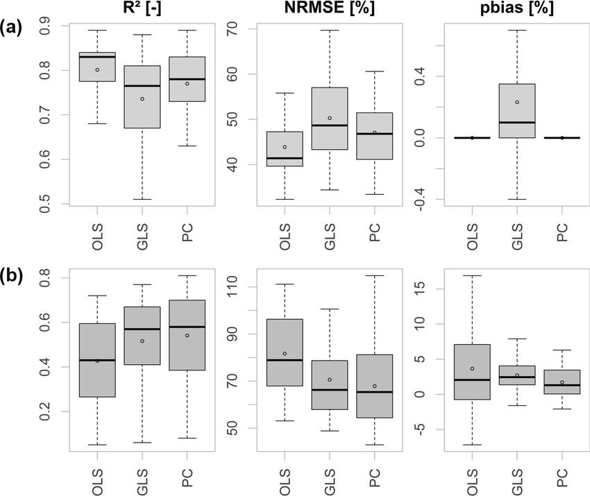
454                           A. Fangmann and U. Haberlandt: Statistical approaches for identification of low-flow drivers

                                                                       Table 5. Median absolute difference in quality criteria between cal-
                                                                       ibration and validation periods for seven stations.

                                                                                          OLS        GLS       PC        HydMod
                                                                              NRMSE       34.4 %     21.4 %    19.3 %    32.7 %
                                                                              PBIAS       6.9 %      8.4 %     7.6 %     3.7 %
                                                                              R2          0.35       0.23      0.23      0.30

                                                                       modeling. Logically, with a changing climate, interrelation-
                                                                       ships between individual meteorological variables and hence
                                                                       the ratio of the influence of individual drivers on low-flow
                                                                       formation will change. At the same time, other forcings and
                                                                       feedbacks may become more or less relevant, which have not
                                                                       been included in the statistical model formulation in the first
                                                                       place. In an initial attempt at encompassing the problem by
                                                                       addressing a potential linear time dependence of the regres-
                                                                       sion coefficients, the parameters have been re-estimated as
Figure 5. Criteria for goodness of fit of different model approaches   linear functions of time using a maximum likelihood fitting.
in the calibration period (a) and validation period (b) over seven     The required complexity of the models has been assessed us-
stations.                                                              ing likelihood ratio tests. However, model fitting appeared
                                                                       problematic for the small calibration period and did not yield
Table 4. Median absolute difference in quality criteria between cal-   an improvement of the existing models.
ibration and validation period for 28 stations.                           It should be noted that the model set up for calibration and
                                                                       validation allows for assessment of changes between directly
                          OLS       GLS       PC                       adjacent periods only. Application of the models to predict
                                                                       low flows in a more distant future under more severe cli-
              NRMSE       37.8 %    20.3 %    20.8 %                   matic change may significantly enhance the error due to non-
              PBIAS       5.1 %     2.7 %     2.7 %
                                                                       stationarity.
              R2          0.37      0.22      0.22
                                                                          Apart from the non-stationary relationship between target
                                                                       variable and regressors, another possible explanation – espe-
                                                                       cially with respect to the observations regarding the hydro-
All quality criteria certify a much better performance during          logical model – could be a significant difference in flow be-
calibration than during validation. Tables 4 and 5 show the            havior between the two periods selected for calibration and
median differences in goodness-of-fit measures for all model           validation, potentially caused by forcings other than the lo-
variants over all stations and over the stations at which hydro-       cal climate. A previous study by Fangmann et al. (2013) has
logical modeling was possible. The differences are severe,             found that time series at a majority of gauges in the study
even though quite a number of precautions have been taken              area are divided by significant break points (according to
during calibration. The R 2 for PC, for example, differs by            Pettitt, 1979) between the years 1987 and 1989. Since nei-
0.22 between calibration and validation. For the seven sta-            ther the hydrological nor the statistical models involve input
tions this difference increases to 0.23. Overfitting appears to        other than the local meteorology, this break cannot be ac-
be an issue, even though the number of regressors has been             counted for by either approach. Also, anthropogenic interfer-
restricted. However, the differences are also observable for           ence poses a relevant factor. Even if indirectly considered in
the hydrological model, in some cases even more drastically            the statistical models, changes in the management patterns
than for the statistical models. The median difference in R 2          would significantly alter the prognosis; a factor that needs to
over the seven stations is 0.3 between calibration and valida-         be considered during model application.
tion periods.                                                             Modeling of the other tested indices showed quite a differ-
   Through separation of the validation period into three parts        entiated picture. As shown exemplarily for seven stations and
it becomes obvious that performance decreases steadily with            the GLS approach in Fig. 7, some indices were reproduced
distance from the calibration period, as shown in Fig. 6.              more successfully (top) and others less so (bottom) than the
Compared are the estimated and the observed means for all              NM7Q. Estimation of the Q95 appeared slightly better in
statistical methods. The effect shows that non-stationary re-          terms of all quality criteria. The Dmax was modeled effec-
lationships between low-flow and meteorological indices are            tively via GLS in terms of R 2 and NRMSE (median values
of major relevance and need to be considered in statistical            of 0.54 % and 80.8 %), but showed quite a large bias. Vmax

Hydrol. Earth Syst. Sci., 23, 447–463, 2019                                            www.hydrol-earth-syst-sci.net/23/447/2019/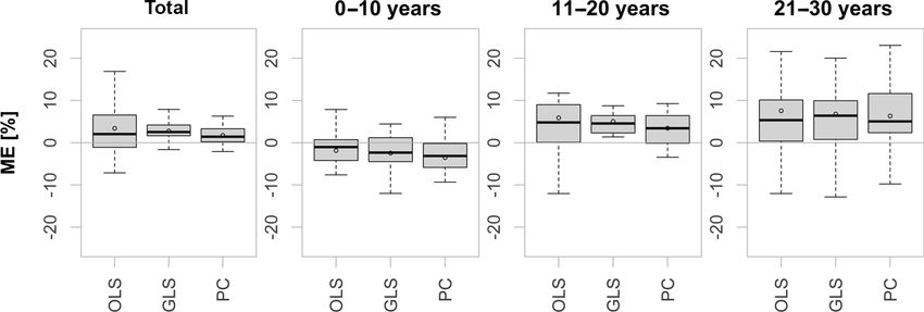
A. Fangmann and U. Haberlandt: Statistical approaches for identification of low-flow drivers                                       455

Figure 6. Mean deviation of estimated from observed means for the whole validation period (left), as well as the first, second and final
10 years of validation.

and especially the annual low-flow timing could not be mod-           volume-based indices. Still, the differences in performance
eled successfully by any of the statistical approaches (median        for the individual indices are visible also for the hydrological
R 2 of 0.31 and 0.03, respectively).                                  models.
   It was noted that the overall model performance was                   It should be noted that the selected statistical methods ex-
slightly higher for the more average values, i.e., NM30Q and          clusively take linear relationships between target variable and
Q80 , than for the more extreme indices NM7Q and Q95 . The            regressors into account. It appears that these linear depen-
median R 2 values of the NM7Q and the NM30Q compare                   dencies are strong, and major portions of the variance in the
as 0.47 and 0.52, the ones of the Q95 and Q80 as 0.49 and             target variables could be explained by the fitted models. At
0.62. Compared to the Dmax and Vmax , the annual average              this point it cannot be precluded that nonlinear relationships
Dmean and Vmean cannot be predicted by the fitted models.             with some meteorological indices do exist, but it is presumed
The validation yields R 2 values below 0.1 for both cases.            that important influential quantities can be linearly related
   The differences in reproducibility of the various metrics          to the target variable. It is well considered that such rela-
can be explained by the nature of the indices and the structure       tionships may change under future conditions that deviate
of the statistical models. The regression model uses aggre-           strongly from the present circumstances under which the sta-
gated meteorological features over a specific period of time          tistical models were fitted. As discussed above, the statistical
for prediction of a desired low-flow variable. The shorter the        models can only be evaluated in a validation period directly
required period, the lower the degree of averaging and the            adjacent to the calibration. Most hydrological models, which
greater the possibility of capturing extremes that cause a sub-       involve much greater detail in physical process representa-
sequent low-flow event. Therefore, indices related to a spe-          tion, will more certainly be transferable to situations where
cific event, like the NM7Q or the Dmax , can be modeled quite         interrelationships between low flow, meteorology, and other
effectively based on previous meteorological states. The fact         influencing factors are altered. The actual capability of the
that more average indices like NM30Q and Q80 are repro-               statistical approaches in estimating future low flow as mere
duced better than more extreme ones can be explained by the           functions of future climate would need to be assessed, e.g.,
same principle. Meteorological indices computed for longer            using simulation studies involving “past” and “future” runoff
base periods are required to model more average index val-            simulated by a hydrological model. Such an experiment is
ues. Errors that occur if extremes cannot be explained by ex-         beyond the scope of this study, but may be a useful test for
ternal variables are lower. Dmean and Vmean , however, do not         further studies.
represent averages of single but of multiple events. These
features cannot be captured by small sets of regressors as            4.2   Low-flow drivers
used in this study.
   Alongside the validation results of the statistical models,        The PC models are used to evaluate the selected explana-
those of the hydrological model are presented in Fig. 7. The          tory variables over all stations. For the NM7Q, the majority
indices in the top panels are deduced from the simulation             of models comprise one or two principal components made
runs of the models that were calibrated on the annual NM7Q.           up of two to eight meteorological indices. Many of the se-
In order to better represent the indices related to duration and      lected variables repeat for most of the models. The most
volume, the model used in the bottom panels was calibrated            common predictors of the NM7Q appear to be the aridity
using the annual Vmean as a fitting criterion. One can see            index P / ETP for 3- and 6-month base periods and for 1–4-
that the results for all indices improve for the hydrological         month lead times, as well as the P -ETP for the same peri-
model as expected, due to a more detailed process representa-         ods. The second most frequent regressor is the SPI of var-
tion. This is especially the case for the average duration- and       ious base periods and lead times (0 to 3 months). Upper
                                                                      precipitation quantiles with various base periods and lead

www.hydrol-earth-syst-sci.net/23/447/2019/                                             Hydrol. Earth Syst. Sci., 23, 447–463, 2019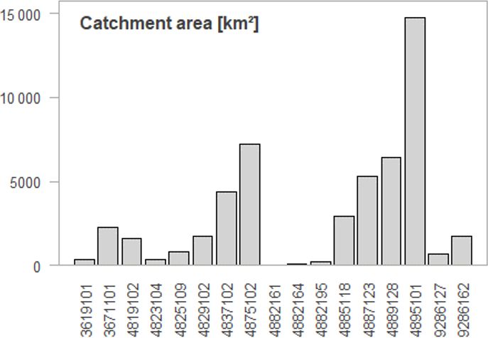
456                          A. Fangmann and U. Haberlandt: Statistical approaches for identification of low-flow drivers

Figure 7. Validation results for the GLS model and the hydrological model for various low-flow indices at seven stations performing better
(a) and worse (b) than for the NM7Q.

times follow in frequency. Several models also contain DSD             erage low-flow values are more easily predicted, apparently
and the ratio between average DSD and WSD as predictors.               requiring less external information. In contrast to the NM7Q,
Pure temperature-based predictors are rare, but do occur in            temperature-based indices do not appear to be important pre-
some cases. The selected lead times of the temperature-based           dictors of the NM30Q. Considering the models of the other
indices are in these cases larger than for the precipitation           indices, it can be seen that the selected regressors differ be-
or water balance indices. Lead times as long as 9 months,              tween the individual types. While Q95 and Q80 are primarily
which would represent November–January temperature, are                predicted by water balance parameters, as are the NM7Q and
observed. Winter temperature hence appears to be an impor-             NM30Q, the models for Dmax and Vmax count a high number
tant predictor for summer low-flow magnitude.                          of indices related to durations, especially average and maxi-
   The inclusion of indices with differing base periods and            mum dry spell duration. The regressors selected for the for-
lead times at the individual stations represents the hetero-           ward and inversed fitting carried out at each station are not
geneity of transformation processes within the study area.             always identical. Some of the independent variables are nat-
One of the major determinants of how meteorological pro-               urally very similar for various base periods and lead times so
cesses translate into flow is catchment size. Larger, rather           that they are almost exchangeable, which in turn makes the
slowly responding catchments with significant storage ca-              fitted models very similar. Still, this observation hints again
pacity will less likely be affected by small meteorological            at the problem of non-stationarity and the observed break-
events and low flows will occur moderated and with signif-             point near the transition between calibration and validation
icant temporal delay. Therefore, statistical models fitted for         periods.
these catchments will most likely include meteorological in-
dices that have been computed for longer base periods and              4.3   Prognosis
lead times. Within small, quickly responding systems on the
other hand, low-flow magnitudes may be related to shorter              For prognosis, the principal component models are applied
dry periods that have occurred recently. Variable selection is         using the ensemble of climate model data described above.
thus carried out in favor of small base periods and lead times.        For reasons of conciseness only the NM7Q is selected as the
Nevertheless, even for smaller catchments an inclusion of              target variable in this example and only changes in the means
temporally leading meteorological indices may mimic initial            for the near- and far-future periods are assessed. In order to
storage conditions and determine the absolute magnitude of             firstly evaluate the climate models’ capabilities to reproduce
a summer low-flow event.                                               the required input variables for the impact models, the mete-
   The models fitted to the NM30Q are comparable to the                orological indices obtained from the models are compared to
ones of the NM7Q but contain on average fewer explana-                 the observation in the reference period. Figure 8 summarizes
tory variables per model. As discussed before, the more av-            the results. Three measures are used to assess the models’ ca-
                                                                       pability to reproduce the indices: (a) the mean error, i.e., the

Hydrol. Earth Syst. Sci., 23, 447–463, 2019                                            www.hydrol-earth-syst-sci.net/23/447/2019/
A. Fangmann and U. Haberlandt: Statistical approaches for identification of low-flow drivers 457
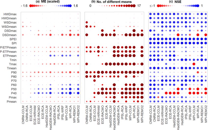
Figure 8. Comparison of simulated and observed meteorological indices for each model over 17 stations: mean error (a), number of signifi-
cant shifts in location (b), and Nash–Sutcliffe efficiency of ordered series (c).
difference in means between simulation and observation over The climate models appear to have limited ability to re-
all stations (computed for scaled data to make it comparable produce some of the true meteorological indices. This effect
between indices); (b) the number of stations where this dif- may be due to the inability of the regional climate models to
ference is significant at a 5 %-significance level, tested using downscale the global climate data appropriately for the study
a non-parametric Mann–Whitney test (Wilcoxon, 1945); and area. One also needs to consider the difference in grid size
(c) the NSE of the simulated and observed index time series, between the observed data, which has a detailed 1 km res-
both ordered by size, as a means of assessing the similarity olution, and the simulation, which is available on a 10 km
of the two distributions. The indices considered in the plot grid. Since mere averaging of the grid cells has been ap-
are calculated on a 6-month base period with a 3-month shift plied to obtain the basin averages, the smoothing effect may
and are representative of most base periods and lead times. be recognizable, especially for small catchments and in het-
The left panel shows that deviations are observed for the erogeneous terrain. The re-calibration technique described in
climatic water balance and the aridity index, i.e., average P - Sect. 3.5 was chosen to address these issues related to various
ETP and P / ETP. The climate models consistently under- forms of scaling.
estimate the observed values. What also becomes apparent Figure 9 shows the prognoses of the individual climate
is that upper precipitation quantiles (P 70–P 90) are mostly models over all stations. Along with the summer NM7Q (bot-
underestimated. The amount of significant differences found tom), projections for the aridity index are shown, as they in-
for the means, especially in P 90, suggest that there is a dicate the overall climatic development. Also, the index is
significant bias throughout the study area. Additionally, the included in numerous stations’ impact models. The index’s
NSE values are rather low, indicating a generally poor repro- development is shown for a 6-month base period without
duction of these index values. Apart from the quantiles and lead time, which equals the computation basis for the NM7Q
the climatic water balance, errors are found for maximum (May–October; center) and a 4-month shift (January–June),
temperature and dry spell durations. The lower precipitation which equals the maximum lead time considered in the sta-
quantiles show quite high errors but are rarely considered in tion models (top).
the station models. For those variables that are considered, The changes for January–June P / ETP are predominantly
additional bias correction may be advisable. positive for the majority of models and stations. Only the
EC-EARTH coupled with the CCLM and the RCA4 show
www.hydrol-earth-syst-sci.net/23/447/2019/ Hydrol. Earth Syst. Sci., 23, 447–463, 2019458 A. Fangmann and U. Haberlandt: Statistical approaches for identification of low-flow drivers
Figure 9. Projected changes in winter (a) and summer (b) aridity index and NM7Q (c) by all models over 17 stations and two future periods.
negative trends. The total range of projections is −13.31 % For the NM7Q the spread of changes over the considered
to +34.10 % in the far-future period. The positive change in stations is significantly larger and increases further from the
the ratios is caused by a significant increase in January–June near- to far-future periods. This is a logical consequence,
precipitation amounts, projected for all stations by all cli- since flow behaves much more heterogeneously throughout
mate models, which exceeds the simultaneously projected in- space and direction and magnitude of change may greatly de-
crease in evapotranspiration. For summer, the projections for pend on local conditions. Overall, the changes in the NM7Q
the P / ETP are more ambiguous. Nine ensemble members appear to be a mixture of the patterns observed for P / ETP
clearly predict a significant decline in the far future, while in both summer and winter. The highest increase in NM7Q
five models project an increase at all considered stations. The is predicted by the IPSL-WRF331F model chain (median
spread of the projection is accordingly large, ranging from 48.18 %), which also shows highest increase in precipitation
−25.75 % to +48.91 %. The IPSL-WRF331F thereby shows amounts and strongest decrease in evapotranspiration in both
by far the highest positive development and can potentially summer and winter. EC-EARTH-CCLM and –RCA4 pre-
be considered an outlier. The rather negative trend in the dict the strongest decrease (median −7.9 % and −13.42 %,
summer P / ETP is related to both decreasing precipitation, respectively), which is also in accordance with declining
as projected by most models, and increasing evapotranspira- P / ETP in both summer and winter. Apart from these mod-
tion. els, there appears to be a general increase projected for sum-
mer NM7Q over the majority of stations. It seems that on av-
Hydrol. Earth Syst. Sci., 23, 447–463, 2019 www.hydrol-earth-syst-sci.net/23/447/2019/A. Fangmann and U. Haberlandt: Statistical approaches for identification of low-flow drivers 459
dicted directions of change are quite unambiguous over the
majority of climate models, and projections are accordingly
quite robust. Exceptions are stations 4819102, 4882195, and
9286162, where the median change is close to 0. What also
becomes apparent in these plots is the spatial dependence be-
tween stations. Identical leading digits of the station numbers
indicate that stations belong to the same river basin, while in-
creasing numbers indicate more downstream locations, i.e.,
larger size, as depicted in Fig. 12. The projected changes are
obviously strongly related to catchment area, since contin-
uous transitions are observable from most negative/smallest
change in NM7Q at the smallest to most positive change at
the largest catchments within each basin. Summer low flow
in catchments with large storage capacity will more likely
be influenced by the increasing annual and winter precipi-
tation amounts, while the flow in the smaller catchments is
more drastically influenced by drier summer meteorological
conditions. It remains to be analyzed, e.g., via hydrological
modeling, whether this observation is an artifact created by
oversimplification of the statistical approaches (through ne-
glect of other relevant, potentially counteracting factors) or a
truly observable phenomenon. Nonetheless, the coherence of
Figure 10. Medians of projected changes in winter (a) and summer
the projected station means suggests that the statistical mod-
(b) aridity index and NM7Q (c) by for individual stations over 15 els – even though they have been fitted independently for ev-
climate models and two future periods. ery station – exhibit a meaningful spatial consistency within
the region. Apparent outliers are not produced by any sta-
tions’ statistical impact model.
The significant increase in winter and partly projected de-
erage the influence of spring and winter meteorological states crease in summer P / ETP may suggest a temporal shift
weighs stronger on the formation of summer NM7Q than the in minimum flows from summer/early fall to late fall/early
actual summer conditions. winter in the study area. In order to test this hypothesis,
Figure 10 shows the spatial distribution of the projected statistical models are fitted to additionally model the win-
changes for the two future periods and the variables analyzed ter NM7Q. Modeling of the winter values was more diffi-
previously. Depicted are the median changes over all climate cult than of the summer low flows since their causes may
model ensemble members for the individual stations. All sta- not be representable by the utilized indices (e.g., water re-
tions show an average increase in winter P / ETP ranging tention by snow). The final projections in Fig. 13 suggest
from +6.84 % to +14.75 % in the far future. At the major- that the expected developments for winter are less conclu-
ity of stations a decrease is projected for summer, with the sive than for summer. At most stations mostly positive trends
largest changes occurring in the Harz mountains, i.e., the are projected for both future periods with lacking robust-
most southeastern stations in the study area, with an aver- ness. A pronounced pattern of change contrasting the sum-
age decrease of −4.72 %. Positive changes can be found in mer NM7Q cannot be observed. Accordingly, with overall
the northern stations, with up to +3.12 % in the near future increasing precipitation amounts, the intensities of the sever-
but decreasing to +2.76 % in the latter period. The NM7Q is est events of the year are expected to decrease at most sta-
projected to increase by up to 22.79 % at all but four stations, tions in the area, regardless of their time of occurrence.
where a median decrease of up to −12.01 % is projected. Still, the findings indicate that there might be a slight de-
Two of these stations are situated in or near the Harz moun- lay in the onset of future low-flow events. The ratio of winter
tains, where flow-forming processes and climate are quite to summer low flows appears to increase slightly at most sta-
different from the rest of the study area. Additionally, their tions, while for the observation 10.20 % of the annual lowest
areas are the smallest in the data set considered for impact low-flow events occur in winter, the models predict on aver-
analysis (44.5 to 363.0 km2 ). Apparently, the NM7Q in these age 15.1 % for the reference period, 20.00 % for the near and
areas is influenced more by summer meteorology than the 22.67 % for the far future.
rest of the study area. A comparison of the signals projected in this work to other
Finally, Fig. 11 shows boxplots for all stations and the pro- studies that analyze comparable regions and climate model
jected changes in the NM7Q over all considered ensemble ensembles but use hydrological models for impact assess-
members. It can be seen that at most of the stations the pre- ment is difficult, due to differences in scale, model ensem-
www.hydrol-earth-syst-sci.net/23/447/2019/ Hydrol. Earth Syst. Sci., 23, 447–463, 2019460 A. Fangmann and U. Haberlandt: Statistical approaches for identification of low-flow drivers
Figure 11. Projected changes in summer NM7Q for individual stations over 15 climate models and two future periods.
central western and northern Europe the projected changes in
streamflow drought under an RCP8.5 scenario appear to dif-
fer between the two hydrological models they applied, both
in direction and magnitude. In general, it appears difficult
to assess future low-flow development in the region, espe-
cially in comparison to the parts of Europe where expected
changes in precipitation are more pronounced and unequivo-
cal between climate models.
5 Conclusions and outlook
The aim of this work was to assess key low-flow drivers us-
ing simplified statistical approaches. Several regression mod-
Figure 12. Catchment areas of the considered gauges. els with varying restrictions and assumptions have been set
up and evaluated in a split-validation procedure. In order to
assess potential future changes in the low flow, the models
ble, and type of analysis (e.g., based on degree of heat- are applied to an ensemble of climate model data. The main
ing rather than on fixed periods). A regional study that is findings are the following.
comparable to this work has been carried out by Osuch et
al. (2017) for Poland. They investigated climate change im- – Modeling of low-flow values as a function of meteo-
pacts on low flows, including the annual NM7Q, using the rological indices appears feasible. An approach using
HBV model and, among others, an RCP8.5 climate model just a few principal components of several variables as
ensemble. They found significant positive changes in the regressors yields the best results for the 60-year obser-
NM7Q for the RCP8.5 scenario, with a more than average vation period. It showed to simultaneously countervail
40 % increase in the study area in a period from 2071 to 2100. problems with multicollinearity and omittance of im-
These changes are much larger than the ones found in this portant explanatory variables.
study but are obtained for a more continental climate. Other
studies analyzing climate change effects on low flows over – Non-stationarity within the relationship between mete-
the whole of Europe (e.g., Marx et al., 2018) or global stud- orological predictors and low-flow target variables ap-
ies (e.g., Wanders and Yada, 2015) using RCP emission sce- pears to be an issue, resulting from the entire neglect of
narios usually find inconclusive changes in low-flow magni- physical processes and changing interrelationships be-
tude for the northwestern parts of Germany (between −10 % tween explanatory metrics. This problematic needs to
and +10 %). The average changes in the annual NM7Q over be considered, when applying the models to future data,
all stations and ensemble members obtained in this study are especially in terms of parameter stability. Ideally the
+5.62 % for the near- and +8.96 % for the far-future periods, models should be revised through inclusion of methods
and are thus within the range of these findings. Van Vliet et to map potential non-stationary processes and interrela-
al. (2015) show in their Europe-wide study that especially in tionships.
Hydrol. Earth Syst. Sci., 23, 447–463, 2019 www.hydrol-earth-syst-sci.net/23/447/2019/A. Fangmann and U. Haberlandt: Statistical approaches for identification of low-flow drivers 461
Figure 13. Projected changes in winter NM7Q for individual stations over 15 climate models and two future periods.
– More average low-flow indices are reproduced better by stead of the observation can potentially help increase the
the statistical models than their more extreme counter- quality of the projections made by the statistical models.
parts, e.g., the NM30Q compared to the NM7Q. Max-
imum duration and deficit volume can be adequately There are potential advantages to applying statistical ap-
modeled, while the onset of an event can by no means proaches that have not been discussed before. One is that
be predicted by the suggested models. the required input consists of variables that are lumped over
a significant amount of time (3–12 months). Such averages
– The main drivers for all low-flow characteristics are
can potentially be better reproduced by climate models than
metrics related to precipitation and evapotranspiration
the daily variability required for other impact model types.
amounts. Temperature indices appear to be relevant at
Also, the statistical models may be easily extended to in-
some stations for certain low-flow metrics. Usually base
clude other forcings like large-scale phenomena, which may
periods for computation and lead times of the explana-
be similarly described by indices like local meteorological
tory variables considered in the station models depend
conditions. Land-use feedbacks also might be includable to
greatly on catchment size and response time of the
some extent. What remains difficult to achieve is to statis-
catchments.
tically model feedbacks between different external variables
– The hydrological model outperforms the statistical ap- with the simplified approaches. This problem may however
proaches, when explicitly calibrated on the low-flow be moderated by including non-stationary regression coeffi-
events. cients for individual variables. Considering issues with the
coupling of global and regional climate and impact models
– Both the statistical and the hydrological model show a (e.g., Dai et al., 2013; Wilby and Harris, 2006), including
major discrepancy in their performances between the issues with downscaling, a direct use of large-scale telecon-
calibration and the validation periods. This indicates a nections, and the possibility of applying the models directly
lack in capturing non-stationary processes or the pres- to extrapolated climate data – rather than just climate model
ence of a significant non-homogeneity between the cal- data – may suggest that statistical approaches can signifi-
ibration and validation period considered for analysis. cantly increase the robustness of predictions. This is espe-
– Applying the principal component model with an en- cially relevant when considered in an ensemble of various
semble of coupled global and regional models based on model types and information sources, as suggested by Laaha
an RCP 8.5 scenario yields on average an increase in et al. (2016) for proper assessment of climate change impacts
summer NM7Q at most stations. Only two small head- on low flows.
water catchments show a decrease in NM7Q in the far The statistical approach can also make use and benefit
future. These stations appear to not be influenced by from inclusion of spatial information, especially with respect
preceding winter precipitation. to regional climate change impact analysis. According to the
concept of “trading space for time”, simultaneous analysis of
– A major weakness of the proposed model type is the all information in an area instead of a single-site approach
reproduction of meteorological indices by the climate will yield more robust parameter estimates and allow for es-
models. However, underestimation of the climatic water timation of climate change signals at unobserved sites. Ex-
balance and upper precipitation quantiles may be a like- tensions of the existing station models using different ap-
wise limiting factor within process-based impact mod- proaches of non-stationary regional frequency analysis have
els. A direct calibration using climate model data in- been proposed in Fangmann (2017). The simultaneous con-
www.hydrol-earth-syst-sci.net/23/447/2019/ Hydrol. Earth Syst. Sci., 23, 447–463, 2019You can also read