SASI Model Description - Working Paper 08/01 Michael Wegener Spiekermann & Wegener Urban and Regional Research
←
→
Page content transcription
If your browser does not render page correctly, please read the page content below
Spiekermann & Wegener
Urban and Regional Research

Working Paper 08/01

Michael Wegener
SASI Model Description

Dortmund, March 2008
Revised August 2008
2

Spiekermann & Wegener
Urban and Regional Research (S&W)
Lindemannstrasse 10
D-44137 Dortmund
E-mail: suw@spiekermann-wegener.de
http://www.spiekermann-wegener.de/en
3

Table of Contents

1. Introduction ........................................................................................................................    4

2. Theoretical Approach ........................................................................................................            5

3. Model Structure .................................................................................................................        7
      3.1 European Developments .........................................................................................                   8
      3.2 Regional Accessibility ..............................................................................................            10
      3.3 Regional GDP .........................................................................................................           11
      3.4 Regional Employment ............................................................................................                 12
      3.5 Regional Population ................................................................................................             13
      3.6 Regional Labour Force ............................................................................................               15
      3.7 Socio-economic indicators .......................................................................................                15

4. Study Area .........................................................................................................................    17
      4.1 Regions ...................................................................................................................      17
      4.2 Networks .................................................................................................................       20

5. Model Data ........................................................................................................................     24
      5.1 Calibration/Validation Data ......................................................................................               24
      5.2 Simulation Data .......................................................................................................          25

6. Model Calibration ...............................................................................................................       26

7. Model Output .....................................................................................................................      28

8. Regional Applications ........................................................................................................          29

9. Future Work .......................................................................................................................     37

References ............................................................................................................................    38

Annex: Model Software .........................................................................................................            42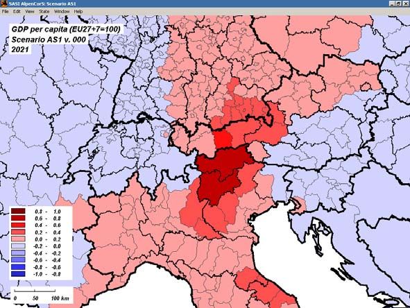
Introduction                                                                                   4

1. Introduction

The regional economic model SASI was developed at the Institute of Spatial Planning of the Uni-
versity of Dortmund since 1996 in co-operation with the Technical University of Vienna in the EU
project SASI (Spatial and Socio-economic Impacts of Transport Investments and Transport Sys-
tem Improvements). A description of the first version of the model is Wegener and Bökemann
(1998). The model has since been applied in several projects for the EU and national and re-
gional authorities, such as
-   IASON: Spatial Economic Effects of Transport Investments and Policies (2001-2003)
-   ESPON 1.1.1: Polycentric Development (2002-2005)
-   ESPON 2.1.1: Territorial Impacts of EU Transport and TEN Policies (2002-2005)
-   ESPON 1.1.3: EU Enlargement (2003-2006)
-   AlpenCorS: Modelling Regional Development in Alpen Corridor South (2004-2005)
-   Impacts of Internalisation of External Costs of Transport in Saxony (2004-2005)
-   STEPS: Scenarios for the Transport System and Energy Supply (2004-2006)
-   SETI: Strategic Evaluation on Transport Investment Priorities 2007-2013 (2005-2006)
-   Ex-ante Evaluation of the TEN-T Multi-Annual Programme 2007-2013 (2007)

The SASI model has been continuously further developed in the course of the projects. Most re-
cent developments include the modelling of generative effects of transport infrastructure invest-
ments and the inclusion of the West Balkan countries into the study area.

This working paper describes the present version of the SASI model.
Theoretical Approach                                                                                 5

2. Theoretical Approach

The important role of transport infrastructure for regional development is one of the fundamental
principles of regional economics. In its most simplified form it implies that regions with better ac-
cess to the locations of input materials and markets will, ceteris paribus, be more productive,
more competitive and hence more successful than more remote and isolated regions (Jochimsen,
1966). However, the relationship between transport infrastructure and economic development
seems to be more complex than this simple model. There are successful regions in the European
core confirming the theoretical expectation that location matters. However, there are also cen-
trally located regions suffering from industrial decline and high unemployment. On the other side
of the spectrum the poorest regions, as theory would predict, are at the periphery, but there are
also prosperous peripheral regions, such as the Scandinavian countries. To make things even
more difficult, some of the economically fastest growing regions are among the most peripheral
ones, such as some regions in the new EU member states.

So it is not surprising that it has been difficult to empirically verify the impact of transport infra-
structure on regional development. There seems to be a clear positive correlation between trans-
port infrastructure endowment or the location in interregional networks and the levels of economic
indicators such as GDP per capita (e.g. Biehl, 1986; 1991; Keeble et al., 1982; 1988). However,
this correlation may merely reflect historical agglomeration processes rather than causal relation-
ships still effective today (cf. Bröcker and Peschel, 1988). Attempts to explain changes in eco-
nomic indicators, i.e. economic growth and decline, by transport investment have been much less
successful. The reason for this failure may be that in countries with an already highly developed
transport infrastructure further transport network improvements bring only marginal benefits. The
conclusion is that transport improvements have strong impacts on regional development only
where they result in removing a bottleneck (Blum, 1982; Biehl, 1986; 1991).

There exists a broad spectrum of theoretical approaches to explain the impacts of transport infra-
structure investments on regional socio-economic development. Originating from different scien-
tific disciplines and intellectual traditions, these approaches presently coexist, even though they
are partially in contradiction (cf. Linnecker, 1997):

- National growth approaches model multiplier effects of public investment in which public invest-
  ment has either positive or negative (crowding-out) influence on private investment, here the ef-
  fects of transport infrastructure investment on private investment and productivity. In general
  only national economies are studied and regional effects are ignored. Pioneered by Aschauer
  (1989; 1993) such studies use time-series analyses and growth model structures to link public
  infrastructure expenditures to movements in private sector productivity. An increase in public
  investment raises the marginal product of private capital and provides an incentive for a higher
  rate of private capital accumulation and labour productivity growth. Critics of these approaches
  argue that there may be better infrastructure strategies than new construction and that policy
  measures aimed at increasing private investment directly rather than via public investment will
  have greater impact on national competitiveness.

- Regional growth approaches rest on the neo-classical growth model which states that regional
  growth in GDP per capita is a function of regional endowment factors including public capital
  such as transport infrastructure, and that, based on the assumption of diminishing returns to
  capital, regions with similar factors should experience converging per-capita incomes over time.
  The suggestion is that, as long as transport infrastructure is unevenly distributed among re-
  gions, transport infrastructure investments in regions with poor infrastructure endowment will
  accelerate the convergence process, whereas once the level of infrastructure provision be-
  comes uniform across regions, they cease to be important. Critics of regional growth models
Theoretical Approach                                                                                6

 built on the central assumption of diminishing returns to capital argue that they cannot distin-
 guish between this and other possible mechanisms generating convergence such as migration
 of labour from poor to rich regions or technological flows from rich to poor regions.

- Production function approaches model economic activity in a region as a function of production
  factors. The classical production factors are capital, labour and land. In modern production
  function approaches, among other location factors, infrastructure is added as a public input
  used by firms within the region (Jochimsen, 1966; Buhr, 1975). The assumption behind this ex-
  panded production function is that regions with higher levels of infrastructure provision will have
  higher output levels and that in regions with cheap and abundant transport infrastructure more
  transport-intensive goods will be produced. The main problem of regional production functions
  is that their econometric estimation tends to confound rather than clarify the complex causal re-
  lationships and substitution effects between production factors. This holds equally for produc-
  tion function approaches including measures of regional transport infrastructure endowment. In
  addition the latter suffer from the fact that they disregard the network quality of transport infra-
  structure, i.e. treat a kilometre of motorway or railway the same everywhere, irrespective of
  where they lead to.

- Accessibility approaches attempt to respond to the latter criticism by substituting more complex
  accessibility indicators for the simple infrastructure endowment in the regional production func-
  tion. Accessibility indicators can be any of the indicators discussed in Schürmann et al. (1997),
  but in most cases are some form of population or economic potential. In that respect they are
  the operationalisation of the concept of 'economic potential' which is based on the assumption
  that regions with better access to markets have a higher probability of being economically suc-
  cessful. Pioneering examples of empirical potential studies for Europe are Keeble et al. (1982;
  1988). Today approaches relying only on accessibility or potential measures have been re-
  placed by the hybrid approaches were accessibility is but one of several explanatory factors of
  regional economic growth, including 'soft' location factors. Also the accessibility indicators used
  have become much more diversified by type, industry and mode (see Schürmann et al., 1997).
  The SASI model is a model of this type incorporating accessibility as one explanatory variable
  among other explanatory factors

- Regional input-output approaches model interregional and inter-industry linkages using the
  Leontief (1966) multiregional input-output framework. These models estimate inter-
  industry/interregional trade flows as a function of transport cost and a fixed matrix of technical
  inter-industry input-output coefficients. Final demand in each region is exogenous. Regional
  supply, however, is elastic, so the models can be used to forecast regional economic develop-
  ment. One example of an operational multiregional input-output models is the MEPLAN regional
  economic model (Echenique, 2004)

- Trade integration approaches model interregional trade flows as a function of interregional
  transport and regional product prices. Peschel (1981) and Bröcker and Peschel (1988) esti-
  mated a trade model for several European countries as a doubly-constrained spatial interaction
  model with fixed supply and demand in each region to assess the impact of reduced tariff barri-
  ers and border delays between European countries through European integration. Their model
  could have been used to forecast the impacts of transport infrastructure improvements on inter-
  regional trade flows. If the origin constraint of fixed regional supply were relaxed, the model
  could have been used also for predicting regional economic development. Krugman (1991),
  Krugman and Venables (1995) and Fujita at al. (1999) extended this simple model of trade
  flows by the introduction of economies of scale and labour mobility. Examples of this type of
  model are the so-called computable general equilibrium (CGE) models (Bröcker, 2004). The
  CGEurope model (Bröcker et al., 2005) is a model of this type.
Model Structure                                                                                  7

3. Model Structure

The SASI model is a recursive simulation model of socio-economic development of regions in
Europe subject to exogenous assumptions about the economic and demographic development of
the European Union as a whole and transport infrastructure investments and transport system
improvements, in particular of the trans-European transport networks (TEN-T).

The SASI model differs from other approaches to model the impacts of transport on regional de-
velopment by modelling not only production (the demand side of regional labour markets) but
also population (the supply side of regional labour markets). A second distinct feature is its dy-
namic network database maintained by RRG Spatial Planning and Geoinformation based on a
'strategic' subset of highly detailed pan-European road, rail and air networks including major his-
torical network changes as far back as 1981 and forecasting expected network changes accord-
ing to the most recent EU documents on the future evolution of the trans-European transport
networks.

The spatial dimension of the model is established by the subdivision of the European Union,
Norway and Switzerland and the Western Balkan countries in 1,330 regions and by connecting
these by road, rail and air networks. For each region the model forecasts the development of
accessibility and GDP per capita. In addition cohesion indicators expressing the impact of trans-
port infrastructure investments and transport system improvements on the convergence (or diver-
gence) of socio-economic development in the regions of the European Union are calculated.

Figure 1 visualises the structure of the SASI model.

                            Figure 1. The structure of the SASI model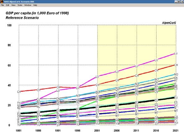
Model Structure                                                                                  8

The temporal dimension of the model is established by dividing time into periods of one year du-
ration. By modelling relatively short time periods both short- and long-term lagged impacts can be
taken into account. In each simulation year the seven submodels of the SASI model are proc-
essed in a recursive way, i.e. sequentially one after another. This implies that within one simula-
tion period no equilibrium between model variables is established; in other words, all endogenous
effects in the model are lagged by one or more years.

The SASI model has six forecasting submodels: European Developments, Regional Accessibility,
Regional GDP, Regional Employment, Regional Population and Regional Labour Force. A sev-
enth submodel calculates Socio-Economic Indicators with respect to efficiency and equity.

Figure 2 shows the sequence of the seven submodels:

                              Figure 2. The sequence of submodels

The seven submodels of the SASI model European Developments, Regional Accessibility, Re-
gional GDP, Regional Employment, Regional Population, Regional Labour Force and Socio-
Economic Indicators are described below.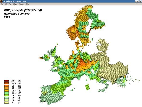
Model Structure                                                                                  9

3.1 European Developments

The European Developments submodel is not a 'submodel' in the narrow sense because it simply
prepares exogenous assumptions about the wider economic and policy framework of the simula-
tions and makes sure that external developments and trends are considered.

For each simulation period the simulation model requires the following assumptions about Euro-
pean developments:

(1) Assumptions about the performance of the European economy as a whole. The performance
    of the European economy is represented by observed values of sectoral GDP for the study
    area as a whole for past years and forecasts for the future years until 2031. All GDP values
    are entered in Euro of 2006.

(2) Assumptions about net migration across Europe's borders. European migration trends are
    represented by observed annual net migration of the study area as a whole for past years
    and forecasts for future years until 2031.

These two groups of assumptions serve as constraints to ensure that the regional forecasts of
economic development and population remain consistent with external developments not mod-
elled in the Reference Scenario. To keep the total economic development exogenous in all sce-
narios would mean that the model would be prevented from making forecasts about the general
increase in production through transport infrastructure investments (generative effects). However,
its parameters are estimated in a way that makes it capable of doing that. Therefore the con-
straints are only applied to the Reference Scenario; by applying the adjustment factors of the
Reference Scenario also to the policy scenarios, the changes in generative effects induced by the
policies are forecast.

(3) Assumptions about transfer payments by the European Union via the Structural Funds and
    the Common Agricultural Policy or by national governments to support specific regions.
    European and national transfer payments are taken into account by annual transfers (in Euro
    of 2006) received by the regions in the European Union during the past and forecasts for fu-
    ture years until 2031.

(4) Assumptions about European integration. The accessibility measures used in the SASI
    model take account of existing barriers between countries, such as border waiting times and
    political, cultural and language barriers. These barriers are estimated for past years since
    1981 and forecast for future years until 2031 taking into account the expected effects of fur-
    ther European integration.

(5) Assumptions about the development of trans-European transport networks (TEN-T). The
    European road, rail and air networks are backcast for the period between 1981 and 2006 in
    five-year increments and forecast in five-year increments until 2031. A policy scenario is a
    time-sequenced programme for addition or upgrading of links of the trans-European road, rail
    and air networks or other transport policies, such as different regimes of social marginal cost
    pricing.

The data for these assumptions do not need to be provided for each year nor for time intervals of
equal length as the model performs the required interpolations for the years in between.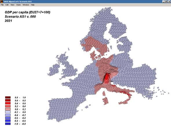
Model Structure                                                                                        10

3.2 Regional Accessibility

The Regional Accessibility submodel calculates regional accessibility indicators expressing the
locational advantage of each region with respect to relevant destinations in the region and in
other regions as a function of the generalised travel cost needed to reach these destinations by
the strategic road, rail and air networks. The model is similar to the accessibility model used in
ESPON (Spiekermann and Schürmann, 2007) but uses generalised cost instead of travel time.

For the selection of accessibility indicators to be used in the model three, possibly conflicting,
objectives were considered to be relevant: First, the accessibility indicators should contribute as
much as possible to explaining regional economic development. Second, the accessibility indica-
tors should be meaningful by itself as indicators of regional quality of life. Third, the accessibility
indicators should be consistent with theories and empirical knowledge about human spatial per-
ception and behaviour.

In the light of these objectives potential accessibility, i.e. the total of destination activities, here
population, Ws(t), in 1,330 internal and 41 external destination regions s in year t weighted by a
negative exponential function of generalised transport cost crsm(t) between origin region r and
destination region s by mode m in year t was adopted:

        Arm (t ) =   ∑W
                     s
                           s   (t ) exp [ − β c rsm (t )]                                              (1)

where Arm(t) is the accessibility of region r by mode m in year t.

Modal generalised transport cost crsm(t) consist of vehicle operating costs or ticket costs based on
cost functions of the SCENES project (Marcial Echenique and Partners, 2000) and costs reflect-
ing value of time. For the latter rail and air timetable travel times and road travel times calculated
from road-type specific travel speeds are used and converted to cost by assumptions about the
value of time of travellers and drivers. Only one common value of time is assumed for the whole
study area, i.e. no distinction is made between the different wage levels and purchasing powers
of countries. The border waiting times mentioned above are converted to monetary cost equiva-
lents. In addition, political, cultural and language barriers are taken into account of as cost penal-
ties added to the transport costs:

                  ′ (t ) + er ′s′ (t ) + s r ′s′ + l r ′s′
        c rsm = c rsm                                        with r ∈ R r '                            (2)

           ′ (t ) is the travel cost between region r and region s in year t including the cost of travel
in which c rsm
time, and er's'(t), sr's' and l r′s′ are exogenous time penalties for political, cultural and language di-
versity in year t between the countries Rr' to which regions r and s belong:

- er's'(t) is a European integration factor reflecting in which supranational structures the two coun-
  tries are, i.e. which political and economic relationship existed between them in year t,
- sr's' is a cultural similarity factor reflecting how similar are cultural and historical experience of
  the two countries.
- l r ′s ′ is a language factor describing the grade of similarity of the mother language(s) spoken in
  the two countries

While the latter two factors are kept constant over the whole simulation, er's'(t) is reduced over
time to account for the effect of European integration. The accessibility indicators used in the
model are not standardised to the European average to show increases in accessibility over time.
Model Structure 11
Modal accessibility indicators are aggregated to one multimodal accessibility indicator expressing
the combined effect of alternative modes by replacing the impedance term crsm(t) by the compos-
ite or logsum impedance:
1
c rs (t ) = −
λ
ln ∑ exp[−λ c rsm (t )]
m∈Mrs
(3)
where Mrs is the set of modes available between regions r and s. Four composite accessibility
indicators are used: accessibility by rail and road for travel, accessibility by rail, road and air for
travel, accessibility by road for freight and accessibility by rail and road for freight.
3.3 Regional GDP
The Regional GDP submodel is based on a quasi-production function incorporating accessibility
as additional production factor. The economic output of a region is forecast separately for the six
economic sectors agriculture, manufacturing, construction, trade/transport/tourism, financial ser-
vices and other services in order to take different requirements for production by each sector into
account. The regional production function predicts annual regional GDP per capita:
q ir (t ) = f [C ir (t ), L ir (t ), A ir (t ), X ir (t ), S r (t ), R ir (t )] (4)
where qir(t) is annual GDP per capita of industrial sector i in region r in year t, Cir(t) is a vector of
capital factors relevant for industrial sector i in region r in year t, Lir(t) is a vector of indicators of
labour availability relevant for industrial sector i in region r in year t, Air is a vector of accessibility
indicators relevant for industrial sector i in region r in year t, Xir(t) is a vector of endowment factors
relevant for industrial sector i in region r in year t¸ Sr(t) are annual transfers received by the region
r in year t and Rir(t) is a region-specific residual taking account of factors not modelled (see be-
low). Note that, even though annual GDP is in fact a flow variable relating to a particular year, it is
modelled like a stock variable.
Assuming that the different production factors can be substituted by each other only to a certain
degree, a multiplicative function which reflects a limitational relation between the factors was cho-
sen. Since this kind of function introduces the coefficients as exponents of the explaining vari-
ables it is possible to interpret the coefficients as elasticities of production reflecting the impor-
tance of the different production factors for economic growth in a sector. The operational specifi-
cation of the regional production functions used in the SASI model is:
α β γ δ ε
q ir (t ) = C ir (t − 5) Lir (t − 1) Air (t − 1) ... X ir (t − 1) ... S r (t − 1) exp( ρ ) R ir (t ) (5)
where qir(t) is GDP per capita of sector i in region r in year t, Cir(t–5) is the economic structure
(share of regional GDP of sector i) in region r in year t–5, Lir(t–1) is a labour market potential indi-
cating the availability of qualified labour in region r and adjacent regions, Air(t-1) is accessibility of
region r relevant for sector i in year t–1, Xir(t–1) is an endowment factor relevant for sector i in
region r in year t–1, Sr(t–1) are transfer payments received by region r in year t–1, Rir(t) is the
regression residual of the estimated GDP values of sector i in region r in year t and α, β, χ, δ, ε
and ρ are regression coefficients.
The ... indicate that depending on the regression results multiple accessibility indicators and en-
dowment indicators can be included in the equation. The economic structure variable is used as
an explanatory variable because the conditions for production in a certain sector depend on the
given sectoral structure, which reflects historic developments and path dependencies not coveredModel Structure 12
by other indicators in the equation. The economic structure variable is delayed by five years as
structural change is a slow process. Endowment factors are indicators measuring the suitability of
the region for economic activity. They include traditional location factors such as capital stock (i.e.
production facilities) and intraregional transport infrastructure as well as 'soft' quality-of-life factors
such as indicators describing the spatial organisation of the region, i.e. its settlement structure
and internal transport system, or institutions of higher education, cultural facilities, good housing
and a pleasant climate and environment. In addition, monetary transfers to regions by the Euro-
pean Union such as assistance by the Structural or Cohesion Funds or the Common Agricultural
Policy or by national governments are considered, as these may account for a sizeable portion of
the economic development of peripheral regions. Regional transfers per capita Sr(t) are provided
by the European Developments submodel (see above).
To take account of 'soft' factors not captured by the endowment and accessibility indicators of the
model, all GDP per capita forecasts are multiplied by a region- and sector-specific residual con-
stant Rir. In the period 1981 to 2001, Rir is the ratio between observed and predicted GDP per
capita of sector i in region r in each year; hence in this period observed sectoral regional GDP is
exactly reproduced by the model. In the period 2002 to 2031, the last residuals calculated for the
year 2001 are applied.
In addition, the results of the regional GDP per capita forecasts are adjusted such that the total of
all regional GDP meets the exogenous forecast of economic development (GDP) of the study
area as a whole by the European Developments submodel (see above). However, these con-
straints are applied only to the reference scenario; in the policy scenarios the adjustment factors
calculated for the reference scenario in each forecasting year are applied. In this way, the
changes in generative effects induced by the policies are forecast.
Regional GDP by industrial sector Qir(t) is then
Qir (t ) = q ir (t ) Pr (t ) (6)
where Pr(t) is regional population (see below).
3.4 Regional Employment
Regional employment by industrial sector is derived from regional GDP by industrial sector and
regional labour productivity.
Regional labour productivity is forecast in the SASI model exogenously based on exogenous
forecasts of labour productivity in each country:
p ir ' (t )
p ir (t ) = p ir (t − 1) with r ∈ R r ' (7)
p ir ' (t − 1)
where pir(t) is labour productivity, i.e. annual GDP per worker, of industrial sector i in region r in
year t, pir ′ (t ) is average labour productivity in sector i in year t in country or group of regions Rr' to
which region r belongs. The rationale behind this specification is the assumption that labour pro-
ductivity by economic sector in a region is predominantly determined by historical conditions in
the region, i.e. by its composition of industries and products, technologies and education and skill
of labour and that it grows by an average sector-specific growth rate.Model Structure 13
Regional employment by industrial sector is then
E ir (t ) = Qir (t ) / p ir (t ) (8)
where Eir(t) is employment in industrial sector i in region r in year t, Qir(t) is the GDP of industrial
sector i in region r in year t and pir(t) is the annual GDP per worker of industrial sector i in region r
in year t.
3.5 Regional Population
The Regional Population submodel forecasts regional population by five-year age groups and sex
through natural change (fertility, mortality) and migration. Population forecasts are needed to rep-
resent the demand side of regional labour markets.
Changes of population due to births and deaths are modelled by a cohort-survival model subject
to exogenous forecasts of regional fertility and mortality rates. To reduce data requirements, a
simplified version of the cohort-survival population projection model with five-year age groups is
applied. The method starts by calculating survivors for each age group and sex:
′ (t ) = Pasr (t − 1) [1 − d asr ′ (t − 1, t )]
Pasr with r ∈ R r ′ (9)
where P'asr(t) are surviving persons of age group a and sex s in region r in year t, Pasr(t–1) is
population of age group a and sex s in year t–1 and d asr ′ (t − 1, t ) is the average annual death rate
of age group a and sex s between years t–1 and t in country or group of regions Rr' to which re-
gion r belongs.
Next it is calculated how many persons change from one age group to the next through ageing
employing a smoothing algorithm:
′ (t ) + 0.08 Pa′+1sr (t )
g asr (t − 1, t ) = 0.12 Pasr for a = 1, 19 (10)
where gasr(t–1,t) is the number of persons of sex s changing from age group a to age group a+1
in region r. Surviving persons in year t are then
′ (t ) + g a −1sr (t − 1, t ) − g asr (t − 1, t )
Pasr (t ) = Pasr for a = 2, 19 (11)
with special cases
P20sr (t ) = P20′ sr (t ) + g 19sr (t − 1, t ) (12)
P1sr (t ) = P1′sr (t ) + Bsr (t − 1, t ) − g 1sr (t − 1, t ) (13)
where Bsr(t–1,t) are births of sex s in region r between years t–1 and t:
10
Bsr (t − 1, t ) = ∑ 0.5 [Pa′2r (t ) + Pa 2r (t )]
a=4
basr ′ (t − 1, t ) [1 − d 0sr ′ (t − 1, t )] with r ∈ R r ′ (14)
where basr ′ (t − 1, t ) are the average number of births of sex s by women of child-bearing five-year
age groups a, a = 4, 10 (15 to 49 years of age) in country or group of regions Rr' to which region rModel Structure 14
belongs between years t–1 and t, and d 0sr ′ (t − 1, t ) is the death rate during the first year of life of
infants of sex s in country or group of regions Rr' to which region r belongs. The exogenous fore-
casts of death and birth rates in the above equations are national rates.
Migration within the European Union and immigration from non-EU countries is modelled in a
simplified migration model as annual regional net migration as a function of regional indicators
expressing the attractiveness of a region as a place of employment and a place to live to take into
account both job-oriented migration and retirement migration:
⎛ q (t − 3 ) ⎞ ⎛ v (t − 3 ) ⎞
m r (t ) = α ⎜⎜ r − 1.5 ⎟⎟ + β ⎜⎜ r − 1.5 ⎟⎟ (15)
⎝ q (t − 3 ) ⎠ ⎝ v (t − 3 ) ⎠
The attractiveness of a region as a place of employment is expressed as the ratio of regional
GDP per capita qr(t–3) and average European GDP per capita . The attractiveness of a region as
a place to live is expressed as the ratio of the regional quality of life vr(t–3) and average Euro-
pean quality of life. Both indicators are lagged by three years to take account of delays in percep-
tion. The forecasts of regional net migration are adjusted to comply with total European net migra-
tion forecast by the European Developments submodel.
In a recent still experimental version of the migration model (ESPON 1.4.4, 2007) not regional
migration balances (net migration) but interregional migration flows are explicitly modelled using
an interregional push-and-pull migration model, in which the push and pull factors are the same
as the ones used in the net migration model shown above plus a third indicator, population den-
sity pr(t-3), expressing the trend of depopulation of remote, thinly populated regions.
Specific assumptions are made to take account of barriers to migration between some old mem-
ber states and the new member states and between EU member states and non-EU countries,
such as restrictions on immigration from certain countries as well as cultural and language barri-
ers to take account of the fact that migrations between two regions in different countries are much
less frequent than migrations between otherwise identical regions in the same country. These
barriers were defined in analogy to the barriers to trade and travel assumed in ESPON 2.1.1
(Bröcker et al., 2005). In addition, airline distance between regions is included as a barrier to mi-
gration. Migration flows between regions r and s are then
M rs (t ) = Pr (t ) E s (t ) g rs (t − 3) exp [− α brs (t )] exp ( − β d rs ) (16)
with
γ δ ε
⎛ q (t − 3 ) ⎞ ⎛ v r (t − 3 ) ⎞ ⎛ p r (t − 3 ) ⎞
g rs (t − 3) = ⎜⎜ r ⎟⎟ ⎜⎜ ⎟⎟ ⎜⎜ ⎟⎟ (17)
⎝ q s (t − 3 ) ⎠ ⎝ v s (t − 3 ) ⎠ ⎝ ps (t − 3 ) ⎠
where Pr(t) is the population in region r in year t, Er(t) are jobs in region r in year t, qr(t-3) is GDP
per capita in region r in year t-3, vr(t-3) is quality of life in region r in year t-3, pr(t-3) is population
density in region r in year t-3, brs(t) are barriers to migration between regions r and s in year t and
drs is airline distance between regions r and s.
Regional educational attainment, i.e. the proportion of residents with higher education in region r,
is forecast exogenously assuming that it grows as in the country or group of regions to which
region r belongs:
hr (t ) = hr (t − 1) hr ′ (t ) / hr ′ (t − 1) with r ∈ R r ′ (18)Model Structure 15
where hr(t) is the proportion of residents with higher education in region r in year t, and hr ′ (t ) is
the average proportion of residents with higher education in country or group of regions Rr' to
which region r belongs.
3.6 Regional Labour Force
The regional labour force is derived from regional population and regional labour force participa-
tion.
Regional labour force participation by sex is partly forecast exogenously and partly affected
endogenously by changes in job availability or unemployment. It is assumed that labour force
participation in a region is predominantly determined by historical conditions in the region, i.e. by
cultural and religious traditions and education and that it grows by an average country-specific
growth rate. However, it is also assumed that it is positively affected by availability of jobs (or
negatively by unemployment):
l sr (t ) = l sr (t − 1) l sr ′ (t ) / l sr ′ (t − 1) − ϕ s u r (t − 1) with r ∈ R r ′ (19)
where l sr (t ) is labour force participation, i.e. the proportion of economically active persons of sex
s of regional population of sex s 15 years of age and older, in region r in year t, l sr ′ (t ) is average
labour participation of sex s in year t in country or group of regions Rr' to which region r belongs,
ur(t–1) is unemployment in region r in the previous year t–1 (see below), and ϕ s is a linear elas-
ticity indicating how much the growth in labour productivity is accelerated or slowed down by re-
gional unemployment. Because at the time of execution of the Regional Labour Force submodel
regional unemployment in year t is not yet known, unemployment in the previous year t–1 is used.
Regional labour force by sex s in region r, Lsr(t), is then
Lsr (t ) = Psr (t ) l sr (t ) (20)
where Psr(t) is population of sex s 15 years of age and older in region r at time t and l sr (t ) is the
labour force participation rate of sex s in region r in year t.
Regional labour force is disaggregated by skill in proportion to educational attainment in the re-
gion calculated in the Regional Population (see above):
Lsr 1 (t ) = hr (t ) Lsr (t ) (21)
with Lsr1(t) being skilled labour and the remainder unskilled labour:
Lsr 2 (t ) = Lsr (t ) − Lsr 1 (t ) (22)
3.7 Socio-economic Indicators
From regional accessibility and GDP per capita forecast by the model equity or cohesion indica-
tors describing their distribution across regions are calculated. Cohesion indicators are macro-
analytical indicators combining the indicators of individual regions into one measure of their spa-
tial concentration. Changes in the cohesion indicators predicted by the model for future transport
policies reveal whether these policies are likely to reduce or increase existing disparities in ac-
cessibility and GDP per capita between the regions.Model Structure 16 In the SASI model five cohesion indicators are calculated: - Coefficient of variation. The coefficient of variation is the standard deviation of region indicator values expressed in percent of their European average. The coefficient of variation informs about the degree of homogeneity or polarisation of a spatial distribution. A coefficient of varia- tion of zero indicates that all areas have the same indicator values. The different size of regions is accounted for by treating each area as a collection of individuals having the same indicator value. The coefficient of variation can be used to compare two scenarios with respect to cohe- sion or equity or two points in time of one scenario with respect to whether convergence or di- vergence occurs. - Gini coefficient. The Lorenz curve compares a rank-ordered cumulative distribution of indicator values of areas with a distribution in which all areas have the same indicator value. This is done graphically by sorting areas by increasing indicator value and drawing their cumulative distribu- tion against a cumulative equal distribution (an upward sloping straight line). The surface be- tween the two cumulative distributions indicates the degree of polarisation of the distribution of indicator values. The Gini coefficient calculates the ratio between the area of that surface and the area of the triangle under the upward sloping line of the equal distribution. A Gini coefficient of zero indicates that the distribution is equal-valued, i.e. that all areas have the same indicator value. A Gini coefficient close to one indicates that the distribution of indicator values is highly polarised, i.e. few areas have very high indicator values and all other areas very low values. The different size of areas can be accounted for by treating each area as a collection of indi- viduals having the same indicator value. - Geometric/arithmetic mean. This indicator compares two methods of averaging among obser- vations: geometric (multiplicative) and arithmetic (additive) averaging. If all observations are equal, the geometric and arithmetic mean are identical, i.e. their ratio is one. If the observations are very heterogeneous, the geometric mean and hence the ratio between the geometric and the arithmetic mean go towards zero. - Correlation between relative change and level. This indicator examines the relationship be- tween the percentage change of an indicator and its magnitude by calculating the correlation coefficient between them. If for instance the correlation between the changes in GDP per capita of the region and the levels of GDP per capita in the regions is positive, the more affluent re- gions gain more than the poorer regions and that disparities in income are increased. If the cor- relation is negative, the poorer regions gain more than the rich regions and disparities de- crease. - Correlation between absolute change and level. This indicator is constructed as the previous one except that absolute changes are considered. This indicator expresses absolute conver- gence or divergence. The results differ substantially from the correlation between relative change and level. If, for instance, two regions, a rich and a poor region, both gain (or lose) ten percent of the GDP per capita in relative terms, in absolute terms the richer region gains (loses) much more than the poorer region.
Study Area                                                                                            17

4. Study Area

The study area of the model are the 27 countries of the European Union plus Norway and Swit-
zerland and the western Balkan countries Albania, Bosnia-Herzegovina, Croatia, FYR Makedonia
and Yugoslavia.

4.1 Regions

The SASI model presently forecasts accessibility and GDP per capita of 1,330 NUTS-3 or equiva-
lent regions in the study area. (see Figure 3). All historical data since 1981 were converted to
NUTS-3 regions of 2003 based on Eurostat information or estimates. These 1,330 regions are the
'internal' regions of the model. The remaining European countries, including the European part of
Russia, are the 'external' regions, which are used as additional destinations when calculating
accessibility indicators. The presently used system of regions is presented in Table 1:

Table 1. SASI model regions

         EU member states             Other internal regions                 External regions

         Country            No.           Country         No.               Country             No.

 Austria                     35   Switzerland                  26   Belarus                       6
 Belgium                     43   Norway                       19   Iceland                       1
 Bulgaria                    28   Albania                       1   Liechtenstein                 1
 Cyprus                       1   Bosnia Herzegovina            1   Moldavia                      1
 Czech Republic              14   Croatia                       2   Russia                       27
 Germany                    439   FYR Makedonia                 1   Turkey                        1
 Denmark                     15   Serbia/Montenegro             4   Ukraine                       4
 Estonia                      5
 Spain                       50
 Finland                     20
 France                      96
 Greece                      51
 Hungary                     20
 Ireland                      8
 Italy                      103
 Lithuania                   10
 Luxembourg                   1
 Latvia                       6
 Malta                        2
 Netherlands                 40
 Poland                      45
 Portugal                    28
 Romania                     42
 Sweden                      21
 Slovenia                    12
 Slovakia                     8
 United Kingdom             133

 Total                  1,276     Total                        54   Total                        41

Work is underway to convert all model data to the new system of NUTS-3 regions valid since
2008 (Hong, 2008).
Study Area 18
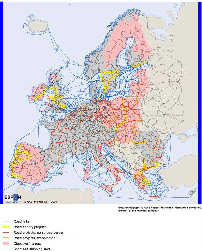
Figure 3. The regions of the SASI model in EuropeStudy Area 19 4.2 Networks The transport networks used by the SASI model originated in the trans-European transport net- work GIS database developed by IRPUD (2003), and now maintained and further developed by RRG (2008). The strategic road, rail and waterways networks used by the SASI model are sub- sets of this database, comprising the trans-European networks specified in Decision 1692/96/EC of the European Parliament and of the Council (European Communities, 1996) and amended in Decision 884/2004 (European Union, 2004), further specified in the TEN Implementation Report (European Commission, 1998) and latest revisions of the TEN guidelines provided by the Euro- pean Commission (1999; 2002a; 2003a) and by the European Communities (2001), information and decisions on priority projects (European Commission, 1995; 1999; 2002b; 2003b; 2004; European Union, 2004), on the TINA networks as identified and further promoted by the TINA Secretariat (1999, 2002), the Helsinki Corridors as well as selected additional links in eastern Europe and other links to guarantee connectivity of NUTS-3 level regions. The strategic air net- work is based on the TEN and TINA airports and other important airports in the remaining coun- tries and contains all flights between these airports (Bröcker et al., 2002) and reflects the state of air travel in 2006. The networks are used to calculate travel times and travel costs between regions and regional accessibility. For that the historical and future developments of the networks are required as input information. The development of the networks over time is reflected in intervals of five years in the database, i.e. the established network database contains information for all modes for the years 1981, 1986, 1991, 1996, 2001, 2006, 2011, 2016 and 2021. For the past period (until 2006) the same network evolution is used for the reference scenario and all scenarios to be evaluated. The scenarios differ in their assumptions about the future network development. Thus, different assumptions about the state of the transport networks in the years 2011, 2016 and 2021 are used for the reference scenario and the scenarios to be evaluated. This means that in contrast to other studies, the simulation of network scenarios is not a matter of ‘with’ or ‘without’ at only one point in time, but that there is gradual network evolution over time. The type of projects and their expected year of completion were taken from the TEN Implementa- tion Report (European Commission, 1998) and the TINA Status Report (TINA Secretariat, 2002) and their most recent revisions (HLG, 2003; European Union, 2004). In case such information was not available in these sources, supplementary information from national ministries or bodies was used as well (for example, the REBIS study (European Commission, 2003c), Europe Aid (2001), or United Nations (1995; 2003). Most projects are composed of different sections with individual project types and completion years. The GIS database set up for this purpose tries to reflect this in that all projects are represented by their individual sections in the database, with individual specifications for type of work and completion year. Only in cases where such detailed information was not available, an overall completion year for all sections of one project was as- signed. Figures 4 and 5 on the following pages show the SASI road and rail networks with the projects studied in ESPON 2.1.1 highlighted (Bröcker et al, 2005). The subsequent Figures 6 and 7 show the current TEN and TINA projects. Figure 6 shows the TEN and TINA priority projects (European Union, 2004). Figure 7 shows all TEN and TINA pro- jects and the priority project corridors (European Union, 2004).
Study Area                                                            20

             Figure 4. The SASI road network (Bröcker et al., 2005)
Study Area 21
Figure 5. The SASI rail network (Bröcker et al., 2005)Study Area 22
Figure 6. TEN and TINA rail and road priority projects (Bröcker et al., 2004)Study Area 23
Figure 7. TEN and TINA road and rail projects and priority corridors (Bröcker et al., 2004)Model Data 24 5. Model Data The data required to perform a typical simulation run with the SASI model can be grouped into base-year data and time-series data. Base-year data describe the state of the regions and the strategic road, rail and air networks in the base year 1981. Time-series data describe exogenous developments or policies defined to control or constrain the simulation. They are either collected or estimated from actual events for the time between the base year and the present or are as- sumptions or policies for the future. Time-series data must be defined for each simulation period, but in practice may be entered only for specific (not necessarily equidistant) years, with the simu- lation model interpolating between them. Exogenous assumptions are required concerning changes in regional labour productivity, re- gional educational attainment and regional labour force participation. All other regional base-year values such as GDP, employment or labour force are calculated by the model. Network data specify the road, rail and air networks used for accessibility calculations, and the evolution of the networks over the simulation period is needed as input. 5.1 Calibration/Validation Data The regional production function in the Regional GDP submodel and the migration function in the Regional Population submodel are the only model functions calibrated using statistical estimation techniques. All other model functions are validated by comparing the output of the whole model with observed values for the period between the base year and the present. Calibration data are data used for calibrating the regional production functions in the Regional GDP submodel and the migration function in the Regional Population submodel. The four years 1981, 1986, 1991 and 1996 are used to gain insights into changes in parameter values over time; however, only the parameter estimates for 2001 are used in the simulation. The calibration data of 1981 are identical with the simulation data for the same year. Regional data (1,330 regions) - Regional GDP per capita by industrial sector in 1981, 1986, 1991, 1996, 2001 - Regional labour productivity by industrial sector in 1981, 1986, 1991, 1996, 2001 - Regional endowment factors in 1981, 1986, 1991, 1996, 2001 - Regional labour force in 1981, 1986, 1991, 1996, 2001 - Regional transfers in 1981, 1986, 1991, 1996, 2001 Network data - Node and link data of strategic road network in 1981, 1986, 1991, 1996, 2001 - Node and link data of strategic rail network in 1981, 1986, 1991, 1996, 2001 - Node and link data of air network in 1981, 1986, 1991, 1996, 2001 Validation data are reference data with which the model results in the period between the base year and the present are compared to assess the validity of the model: Regional data (1,330 regions) - Regional population (by age and sex) in 1981, 1986, 1991, 1996, 2001 - Regional GDP (by industrial sector) in 1981, 1986, 1991, 1996, 2001 - Regional labour force (by sex) in 1981, 1986, 1991, 1996, 2001 - Regional employment (by industrial sector) in 1981, 1986, 1991, 1996, 2001
Model Data                                                                                        25

5.2 Simulation Data

Simulation data are the data required to perform a typical simulation. They can be grouped into
base-year data and time-series data.

Base-year data describe the state of the regions and the strategic transport networks in the base
year and so are either regional or network data. Regional base-year data provide base values for the
Regional GDP submodel and the Regional Population submodel as well as base values for exoge-
nous forecasts of changes in regional educational attainment and regional labour force participation.
Network base-year data specify the road, rail and air networks used for accessibility calculations in
the base year.

Regional data (1,330 regions)
   - Regional GDP per capita by industrial sector in 1981
   - Regional labour productivity (GDP per worker) by industrial sector in 1981
   - Regional population by five-year age group and sex in 1981
   - Regional educational attainment in 1981
   - Regional labour force participation rate by sex in 1981
   - Regional quality-of-life indicators in 1981

Network data
   - Node and link data of strategic road network in 1981
   - Node and link data of strategic rail network in 1981
   - Node and link data of air network in 1981

Time-series data describe exogenous developments or policies defined to control or constrain the
simulation. They are either collected or estimated from actual events for the time between the base
year and the present or are assumptions or policies for the future. Time-series are defined for each
simulation period. All GDP data are converted to Euro of 2006.

European data (34 countries)
   - Total European GDP by industrial sector, 1981-2031
   - Total European net migration, 1981-2031

National data (34 countries)
   - National GDP per worker by industrial sector, 1981-2031
   - National fertility rates by five-year age group and sex, 1981-2031
   - National mortality rates by five-year age group and sex, 1981-2031
   - National educational attainment, 1981-2031
   - National labour force participation by sex, 1981-2031

Regional data (1,330 regions)
   - Regional endowment factors, 1981-2031
   - Regional transfers, 1981-2031

Network data
   - Changes of node and link data of strategic road network, 1981-2031
   - Changes of node and link data of strategic rail network, 1981-2031
   - Changes of node and link data of air network, 1981-2031
Model Calibration                                                                                 26

6. Model Calibration

The regional production functions of the SASI model were estimated by linear regression of the
logarithmically transformed Cobb-Douglas regional production functions for the 1,330 internal
regions and the six industrial sectors used in AlpenCorS for the years 1981, 1986, 1991, 1996
and 2001. The dependent variable is regional GDP per capita in 1,000 Euro of 1998.

Because of numerous gaps and inconsistencies in the data, extensive research was necessary to
substitute missing or inconsistent data by estimation or by analogy with similar regions. In particu-
lar for the accession countries in eastern Europe, which underwent the transition from planned
economies to market economies, information on regional GDP was inconsistent or completely
missing. It was therefore necessary to adjust regional sectoral GDP data for the years 1981 to
1991 to conform to estimates of regional GDP totals by Eurostat. In a similar way the sectoral
composition of regional economies was cross-checked by comparison with the sectoral composi-
tion of gross value added in the Eurostat New Cronos database.

The independent variables of the regressions were a large set of regional indicators of potential
explanatory value from which the following were selected:

     sgdpn          Share of GDP of sector n (%)
     gdpwn          GDP per worker in sector n (1,000 Euro of 1998)
     acctrra        Accessibility travel road/rail/air
     accfrr         Accessibility freight road/rail
     rlmp           Regional labour market potential (accessibility to labour)
     pdens          Population density (pop/ha)
     devld          Developed land (%)
     rdinv          R&D investment (% of GDP)
     eduhi          Share of population with higher education (%)
     quali          Quality of life indicator (0-100)

To take account of the slow process of economic structural change, independent variables sgdpn
and gdpwn are lagged by five years; all other independent variables are lagged by one year, i.e.
the most recent available value is taken. Because no data are available for years before 1981, no
lags are applied for 1981.

Table 2 shows the regression coefficients for the selected variables for 2001. Given the large
number of regions and the exclusion of region size by the choice of GDP per capita as dependent
variable, the results are very satisfactory.

In the simulations for the years 1981 to 2001, predicted GDP values were corrected by their re-
siduals to match observed values. The regression parameters and residuals for 2001 were used
for the simulations for the years 2002 to 2031.
Model Calibration 27
Table 2. SASI model: calibration results (2001)
Regression coefficients
Variables Trade,
Manufac- Construc- Financial Other
Agriculture tourism,
turing tion services services
transport
sgdpn 0.460475 0.762302 0.879101 0.709550 0.716462 1.003335
gdpwn 0.554202 0.881195 0.750888 0.900674 0.784505 0.793632
acctrra 0.034314 0.092961 0.238186
accfrr 0.170935 0.061114 0.149949
rlmp 0.039794 0.029366
pdens –0.107152 0.043427
devld -0.050657 –0.110744
rdinv 0.133867 0.271060 0.125108
eduhi 0.226394 0.297862 0.065298 0.109546
quali 0.052679
Constant –1.819437 –0.921640 –1.530766 –0.623225 -1.077333 -1.565620
2
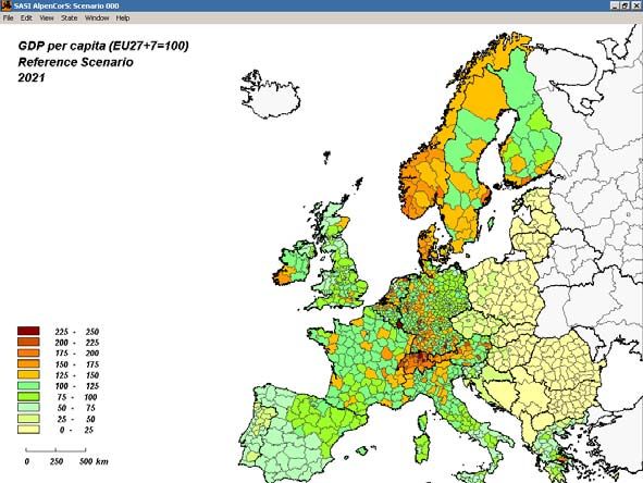
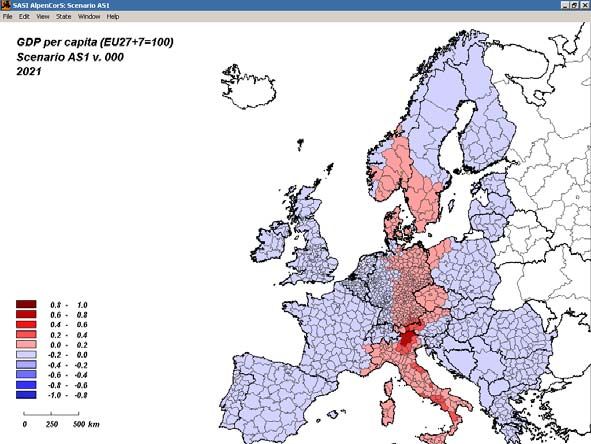
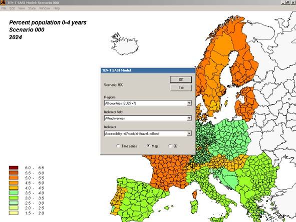
r 0.711 0.692 0.637 0.786 0.830 0.699Model Output 28 7. Model Output The main output of the SASI model are accessibility and GDP per capita for each region for each year of the simulation. However, a great number of other regional indicators are generated during the simulation. These indicators can be examined during the simulation by observing time-series diagrams, choropleth maps or 3D representations of variables of interest on the computer display. The user may interactively change the selection of variables to be displayed during processing. The same selection of variables can be analysed and post-processed after the simulation. The user can compare the results using a comparison programme. The following options can be selected: Population indicators - Population (1981=100) - Percent population 0-5 years - Percent population 6-14 years - Percent population 15-29 years - Percent population 30-59 years - Percent population 60+ years - Labour force (1981=100) - Labour force participation rate (%) - Percent lower education - Percent medium education - Percent higher education - Net migration per year (%) - Net commuting (% of labour force) Economic indicators - GDP (1981=100) - Percent non-service GDP - Percent service GDP - GDP per capita (in 1,000 Euro of 2006) - GDP per capita (EU15=100) - GDP per worker (in 1,000 Euro of 2006) - Employment (1981=100) - Percent non-service employment - Percent service employment - Unemployment (%) - Agricultural subsidies (% of GDP) - European subsidies (% of GDP) - National subsidies (% of GDP) Attractiveness indicators - Accessibility rail/road (travel, million) - Accessibility rail/road/air (travel, million) - Accessibility road (freight, million) - Accessibility rail/road (freight, million) - Soil quality (yield of cereals in t/ha) - Developable land (%) - R&D investment (% of GDP) - Quality of life (0-100)
You can also read