Working Paper Series The effect of public investment in Europe: a model-based assessment - European Central ...

Working Paper Series
 Jasper de Jong, Marien Ferdinandusse, The effect of public investment in
 Josip Funda, Igor Vetlov
 Europe:
 a model-based assessment

 No 2021 / February 2017

Disclaimer: This paper should not be reported as representing the views of the European Central Bank
(ECB). The views expressed are those of the authors and do not necessarily reflect those of the ECB.

Contents
Abstract 2

Non-technical summary 3

1 Introduction 5

2 Government investment and capital stocks: some stylized facts 7

3 Literature overview 12

 3.1 Partial equilibrium effects 12

 3.2 Studies estimating general equilibrium effects 14

4 VAR-based estimates of the effect of public capital on output 18

 4.1 Model selection 18

 4.2 Simulation results 20

5 Structural model-based simulations 23

 5.1 Fiscal sector in EAGLE: an overview 23

 5.2 Model-based scenario analysis 25

 5.3 Alternative sources of financing 26

 5.4 Initial level of capital stock and investment efficiency 28

 5.5 Alternative output elasticity of public capital 29

 5.6 Financing constraints in the private sector 31

 5.7 Monetary policy accommodation 32

 5.8 Cross-border spill-overs and policy coordination 34

6 Conclusions 36

7 References 38

8 Annex 43

Acknowledgements 46

ECB Working Paper 2021, February 2017 1

Abstract

We consider the effect of an increase in public investments on output in Europe
against the background of a sharp drop of public investments in a number of EU
countries during the crisis and subsequent policy discussions on the need to
stimulate public investments. We start with a brief overview of recent developments
in public investments, including some methodological issues, and provide a literature
overview of the effect of public investments on growth. On the basis of updated
estimates of the public capital stock, we estimate the output response to a public
capital impulse, using VAR models. In addition, using a structural model, we
investigate the sensitivity of the macroeconomic impact of an increase in public
investments to alternative assumptions about economic structures and policy
implementations.

Keywords: fiscal policy, public investment, euro area, general equilibrium modelling

JEL codes: E32, E62, C30

ECB Working Paper 2021, February 2017 2

Non-technical summary

Public investment in Europe has significantly declined since the crisis, although
developments are heterogeneous across countries. This has led to calls for
stimulating public investment in an environment of low borrowing costs for
governments, weak economic growth and monetary policy at the lower bound.
Against this background, this paper assesses the output effects of public capital and
investments and discusses the importance of various economic mechanisms
determining the transmission of public investment shocks.

The literature suggests that an increase in public investment has positive demand
effects and can contribute to the economy’s potential output by increasing the stock
of public capital. While the empirical literature on the effect of public capital on output
typically finds a positive effect, estimates vary considerably according to the time
period, country, measure of capital and estimation method. Similarly, the productivity
of public capital may vary over time and could decline. Any increase in public
investment needs to be assessed in the light of its productivity, its financing and the
relative costs and benefits of the financing options.

Using an updated data set of public capital stocks, we provide VAR-based estimates
of the output effects of an increase in the public capital stock in twelve EU countries.
In line with past studies, we find that public capital enhances productivity in most of
the countries included in the sample as the long-run impact of a shock to public
capital on GDP is estimated to be positive. However, even though public investment
expenditures were cut strongly during the recent crisis in many countries with large
consolidation needs, we find no conclusive evidence that the public capital effects on
output are currently larger than before the crisis.

To gain further insights in the effects of public investments on output and public
finances, we simulate a temporary but sustained increase in public investment in a
large euro area economy using a structural model. The simulation results show the
sensitivity of the implied output and budget responses to alternative policy
implementation strategies. First, an increase in public investment will have the
strongest short-term demand effects, including in terms of spillovers to other
countries, with an anticipated accommodative monetary policy. This finding
strengthens the case for increasing public investment in the current low-inflation
environment. Second, a debt or revenue-financed increase in productive public
investment implies significantly larger short-term output gains compared with an
increase in investment financed by cutting other public expenditures. However, when
distortionary taxes, e.g. labour income taxes, are used to finance public investment,
the short-term output gains of additional public investment have to be traded off
against the tax-induced output losses over the longer term, whereas any increase in
public investment financed by higher public debt must be weighed up against
possible fiscal sustainability concerns. Last, the longer-term positive effects on the
economy’s potential output and the impact on public finances crucially depend on the
effectiveness of investment and the productivity of public capital. If these are low, an

ECB Working Paper 2021, February 2017 3

increase in public investment is associated with a greater deterioration of the debt
outlook and less persistent output gains.

In conclusion, to produce positive effects, any recommendation for a public
investment push in the EU must go along with a rigorous selection of projects, to
ensure that the investment is efficient and productive.

ECB Working Paper 2021, February 2017 4

1 Introduction

 Since the start of the global financial crisis, public investment has fallen in a number
 of countries, particularly those that experienced market pressure. Low levels of
 public investment, if maintained over a prolonged period, may lead to a deterioration
 of public capital and diminish longer-term output. The fall in public investment and
 the current low interest rate environment have prompted calls to stimulate public
 investment spending as a way to increase short-term demand and raise potential
 output (see e.g. IMF (2014)). In the European Union (EU), this has led to the
 adoption of the Investment Plan for Europe (2015), the so-called “Juncker plan”. The
 latter aims to stimulate infrastructure and other public investments through
 combining first-risk guarantees for private sector participation, increasing information
 on viable projects, and improving the investment climate. The fiscal positions of
 many EU countries remain fragile, however, and the provisions of the Stability and
 Growth Pact call for further fiscal consolidation in many of them. In this regard, it
 seems to be prudent to take a closer look at the relationship between public
 investment and economic growth as well as budgetary implications of the proposed
 policy.

 Against this background, this paper investigates economic effects of public capital
 and investment utilising both structural and non-structural model-based illustrative
 simulations. First, using the methodology proposed by Kamps (2006) for updating a
 dataset for twelve EU countries, the paper reports new VAR-based estimates of the
 output effects of an increase in public capital stock. 1 Similar to Kamps (2005), we
 find that, for most of the countries included in the sample, the long-run impact of a
 shock from public capital on GDP is estimated to be positive, i.e. public capital
 enhances the production capacity, but not necessarily differently than before the
 crisis.

 Second, to gain further insights in the economic effects of an increase in public
 investment on output and public finances, the paper discusses simulations of a
 temporary but sustained increase in public investment, based on the EAGLE model
 – a multi-country dynamic general equilibrium model (Gomes et al., 2010). An
 increase in public investment is found to increase output both in the short term
 (demand effect) and long term (supply effect), with only a moderate increase in
 government debt or even a decrease if financed by revenue increases or other
 expenditure cuts. However, the debt increases considerably more in cases when the
 existing public capital stock is already high, the productivity of public capital is low or
 the efficiency of investment (e.g. through waste or corruption) is low. The effects are
 also sensitive to the monetary policy stance and cross-border spill-overs also matter.

 Our model-based simulation results reveal that an increase in public investment will
 have the strongest short-term demand effects with a fully anticipated, non-

 1
 Public investment data are subject to limitations in cross-country comparability, e.g. due to differences in
 sector delineation.

 ECB Working Paper 2021, February 2017 5

responsive monetary policy, which argues in favour of undertaking public investment
at the current juncture. However, the longer-term positive effects on the economy’s
potential output and the impact on public finances crucially depend on the
effectiveness of investment and its productive effect. If these are low, an increase in
public investment is associated with a deterioration of the debt outlook. Accordingly,
the recent evolution in public investment or public capital cannot by itself justify a
“one-size fits all” recommendation for an investment push in the EU. Rather, the
evidence presented here underlines the consideration that should be given to a
rigorous selection of investment projects, which should be done on a case-by-case
basis, to ensure that investment is efficient and productive.

The rest of the paper is structured as follows. Some stylized facts about recent
developments in public investments and capital stocks are discussed in section 2.
Section 3 provides a literature overview of the effect of public investment on growth.
Our estimates of the effect of public capital on output are provided in section 4, while
we present simulations of the impact of increasing investment under different
conditions, based on a structural model, in section 5. Section 6 concludes.

ECB Working Paper 2021, February 2017 6

2 Government investment and capital
 stocks: some stylized facts

 In the empirical literature, a common approach to approximate public investment is
 to use statistical data on general government gross fixed capital formation. Public
 capital stock series are typically constructed as the sum of past investments,
 allowing for depreciation. 2 This approach is largely dictated by the required data
 availability. However, is not without caveats, which are mostly related to investment
 measurement issues.

 A general issue with monetary measures of public investment is their ability to
 adequately describe ‘true’ public capital (investments). First of all, the distinction
 between public investment and other government expenditures is not always clear
 with respect to their effect on the productive capacity of the economy. One might
 expect public investments to be more supportive to growth compared to other
 government spending, by increasing the productive capacity of the economy.
 However, some current government expenditures, for example, education and health
 care expenditures, contribute to the building up of a (private) human capital stock,
 thus also enhancing the supply side of the economy and contributing to growth (e.g.,
 Barro (2001) and Sala-I-Martin et al. (2004)). 3 A second issue is that the distinction
 between public and private investment is not always clear. For example, private
 parties often, through private-public partnerships (PPPs), participate in infrastructure
 projects – some of which are classified as public investments. Furthermore,
 privatisation and outsourcing have resulted in public investments being reclassified
 as private (with in some cases subsequent reversals). A third issue is inefficiency or
 corruption which can reduce the economic impact of public investments. This is a
 relevant consideration, since the quality of public governance and political checks
 and balances differs widely across countries (Keefer and Knack, 2007). 4 Using
 physical measures of investment or capital stocks 5 can circumvent only some of the
 monetary measurement issues since physical measures also face significant
 limitations (Hulten, 1996): quality measurement issues, comparability across
 countries, etc.

 2
 While the terms general government gross fixed capital formation (GFCF) and public investment (as well
 as general government capital stock and public capital stock) are used throughout this chapter
 interchangeably, these are not the same concepts. As stated in ESA2010 20.303 public sector consists
 of general government and public corporations. Therefore, the general government GFCF potentially
 excludes large part of public sector investments.
 3
 Also, at least part of regular maintenance expenditures will be classified as current expenditures, rather
 than investments.
 4
 Gupta et al. (2014) tackle this issue by constructing an efficiency-adjusted public capital stock, based on a
 public investment management index available for low- and middle income countries (see Dabla-Norris
 et al. (2011)). They find that ignoring public investment inefficiencies leads to an underestimation of
 marginal productivities of both private and public capital.
 5
 A recent example is due to Calderón et al. (2014), who compose a synthetic measure of infrastructure
 comprising transport, power and telecommunications and estimate a production function. Positive
 contributions to economic growth are found in other studies using physical measures of public capital
 as well (e.g., broadband penetration (Czernich et al., 2011); length of roads and railways, number of
 fixed telephone lines and electricity generating capacity (Canning, 1999; Égert et al., 2009)).

 ECB Working Paper 2021, February 2017 7

With these caveats in mind, this paper, in line with the literature, uses the
 conventional measures of government investment as defined in national accounts.
 Charts 1 and 2 show dynamics of public and private investment over time and across
 countries whereas Chart 3 plots developments of the estimated capital stock series
 for EU countries.

Chart 1 Chart 1b
Public investment Private investment

(as a percentage of GDP) (as a percentage of GDP)

 euro area Japan euro area Japan
 United States EU United States EU
7 23

 22

6 21

 20

5 19

 18

4 17

 16

3 15

 14

2 13
 1995 1998 2001 2004 2007 2010 2013 1995 1998 2001 2004 2007 2010 2013

Source: European Commission. Source: European Commission.

Chart 2a Chart 2b
Public investment-to-GDP ratio Public investment-to-government expenditure ratio

(as a percentage of GDP) (as a percentage of government expenditure)

 average 2012-2014 average 2012-2014
 average 1995-2007 average 1995-2007
7 16

6 14

 12
5
 10
4
 8
3
 6

2
 4

1 2

0 0
 FR

 FI
 MT

 LT

 LV
 GR

 IE
 LU

 IT
 CY

 HR

 CZ

 NL

 DE

 UK

 DK

 HU

 RO
 PT

 ES

 SK

 EA

 EU

 BE
 SI
 AT

 EE

 SE

 BG

 PL
 FR

 FI
 MT

 LU

 LT

 LV
 GR

 IE

 IT
 HR

 CY

 CZ

 NL

 DE

 UK

 DK
 HU

 RO
 PT

 ES

 SK

 EA

 EU

 AT
 SE
 BE

 EE

 SI

 BG

 PL

Source: European Commission. Source: European Commission.
Note: Countries ordered by change in average public investment 2012-14 versus Note: Countries ordered by change in average public investment 2012-14 versus
1995-2007. 1995-2007.

 In advanced economies, public investment has declined from around 4% of GDP in
 the 1980s to around 3% by the mid-1990s. This long-term downward trend could be
 attributed to a number of factors. First, this evolution could be related to economic

 ECB Working Paper 2021, February 2017 8

and demographic changes, such as a shift towards less capital intensive production
and more services and the ageing of societies. Second, since public investment is
considered to be among the easiest to cut during consolidation periods, the
downward trend might have been driven by political considerations.

After being stable at the level of around 3% of GDP for more than a decade, general
government investment in the EU increased significantly at the beginning of the crisis
(see Chart 1). This reflected a strong fall in economic activity (denominator effect) as
well as a response of the European governments to a call by the European
Commission for a fiscal stimulus in 2009. However, with consolidation efforts
accelerating from 2010 onwards, public investment expenditures declined rapidly
and reverted to a ratio around the pre-crisis average of 3% of GDP. Private sector
investment, on the contrary, declined primarily in the early years of the crisis but did
not recover. Compared to the peak in 2007, the private investment-to-GDP ratio in
2010 was down by almost 3 pp, and remained more or less constant ever since at a
below pre-crisis level. Developments for the euro area are more or less the same as
for the EU, although public investments are currently somewhat below the pre-crisis
ratio.

The EU average hides substantial differences between individual member states in
terms of developments of public investment (Chart 2). In countries with relatively low
levels of general government investment in the years before the crisis, public
investment generally has not declined much or even increased (e.g., Germany,
Austria, Belgium or Denmark). Public investment generally increased in countries
that benefited from increasing support from EU funds during these years, e.g.,
Latvia, Lithuania, Bulgaria, Poland and Romania. The largest reductions in public
investment ratios took place in countries with high pre-crisis public investment ratios
and in countries with large consolidation needs. Most notably, public investments (as
a percent of GDP) were reduced by more than a fifth in Portugal, Ireland, Spain,
Croatia, Cyprus and Greece. Expressed in terms of government expenditures, the
decline in these countries is even larger reflecting the fact that government
investments were used more intensively than other expenditure items as a
consolidation instrument.

The variation in public investment data thus suggests the existence of substantial
differences in the capital stocks, although cross-country comparisons should be
treated with caution on account of the data and measurement issues mentioned
above. Eventually, it is the capital stock, or more specifically the flow of capital
services it provides, that contributes to sustaining a certain level of potential output.
Assuming decreasing marginal benefits of public capital, one would expect the
highest levels of public investment to prevail in countries with a relatively small public
capital stock. However, direct data on the size of the general government capital
stock are generally not readily available.

Chart 3 presents our estimates of public capital stocks for a selection of European
countries, used later for the empirical analysis. These government capital stock data
are constructed by applying a perpetual inventory method, updating earlier work of

ECB Working Paper 2021, February 2017 9

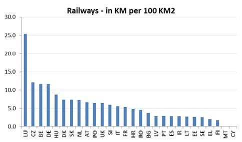
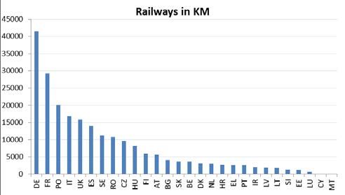
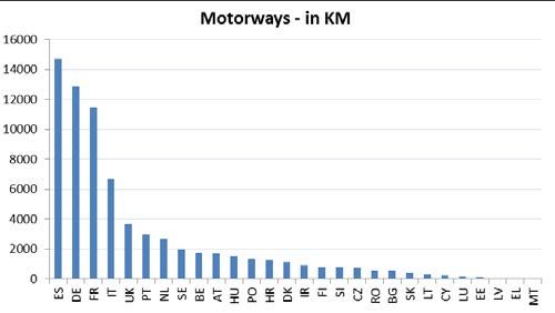
Kamps (2006). 6 As the ESA2010 data on government investment are available only
 from 1995 or later, for this purpose ESA95 data with a reference year 2005 were
 used. While using ESA95 data also avoids including investment in military
 equipment, which are assumed not to be important for the production process, it
 omits spending on R&D that has been included in ESA2010.

Chart 3
Public capital stock, 1960-2014

(percent of GDP; volume)

Notes: authors’ calculations.

 Two observations stand out. First, despite still considerable cross-country
 differences, capital stocks seem to have been converging in size internationally. In
 2014, most of the considered countries had public capital stocks between 25% and
 60% of GDP. There is no apparent relation between the size of the public capital
 stock and GDP per capita. Secondly, in a number of countries, public capital stocks
 (as a ratio to GDP) have actually declined over the last two or three decades,
 reflecting a gradual decline in investment rates. To some extent, this may be the
 result of privatisations and outsourcing of public services which took place in the
 eighties and nineties. Another (statistical) reason could be that expenditures on
 regular maintenance are counted as current expenditures rather than investments.
 Even though, e.g., a road is maintained well, its statistical value would decline over
 time if the applied depreciation rate does not fully incorporate maintenance efforts. In
 any case, it should be clear that these public capital stock measures are necessarily
 only crude proxies for the true public capital stock. Furthermore, since capital is
 valued at production costs, these data do not give us any indication of the quality of
 the public capital stock.

 Physical measures of countries’ infrastructure point to substantial differences in
 levels of public capital (see Annex). The amount of motorways, railways and
 households with internet access vary considerably between countries. Measures of

 6
 It is assumed that the depreciation rate for government capital increases from 2.5% in 1960 to 4.8% in
 2014. The increasing depreciation rate may reflect an increasing weight of assets with relatively short
 asset lives or a shortening of asset lives, which are both characteristic of information and
 communication technology -related assets. Differences in the composition of the capital stock across
 countries are ignored due to lack of data. More details on the calculation of capital stocks, as well as
 the capital stock series themselves, are provided in De Jong et al. (2017) and references therein.

 ECB Working Paper 2021, February 2017 10

physical infrastructure are, not surprisingly, strongly related to country and
population size. At a given population size, larger countries tend to have more
kilometres of roads and railways; likewise, holding country size constant, countries
with larger populations tend to have more kilometres of roads and railways. Of
course, length of networks is only a rough measure of the economic relevance, as it
is not a complete measure of network size (e.g., no distinction is made between a
two-lane and a four-lane motorway), nor does it take the quality of the network into
account. Concerning digital connectivity, income per capita appears to be an
important driver of country differences.

According to survey data, the quality of infrastructure recently improved in most
countries, although there are some exceptions. The World Economic Forum surveys
business executives worldwide on a broad range of economic topics in the context of
its Global Competitiveness Reports (World Economic Forum 2015 and earlier
editions), among which the quality of infrastructure in their respective countries (see
Annex). The World Bank asks international freight forwarders to rate the quality of
trade and transport related infrastructure in countries their companies serve most, as
part of its Logistics Performance Index (World Bank 2014 and earlier editions). Both
surveys show that, overall, the perceived quality of infrastructure in Europe seems to
have improved since 2006/2007. Notable exceptions are Germany, France and
Denmark, where business executives have become less satisfied with infrastructure
quality, albeit from a high level. Satisfaction with the quality of roads has suffered
markedly in these three countries, but there has been a worsening of the perceived
quality of other elements of infrastructure, such as railways, waterways or air
transport infrastructure, as well. Freight forwarders were most critical of
developments in Austria and Finland. Germany, France and Denmark actually
performed similar or even slightly better in 2014 compared to 2007. The conflicting
outcomes on both surveys underline that the survey results should be interpreted
with great caution though.

ECB Working Paper 2021, February 2017 11

3 Literature overview

 There is a substantial, largely empirical, literature aiming to quantify the economic
 importance of public capital. One major branch focuses on partial effects of public
 capital, in particular on the contribution of public capital or investments to either
 output production or cost-reduction. The second major branch of the literature aims
 to provide a broader picture by taking into account feedback effects from higher
 public capital or investments on the rest of the economy. Two common methods for
 incorporating feedback effects are estimation of Vector Autoregressive models
 (VAR) and the use of structural macroeconomic models. This section gives a brief
 overview of some theoretical considerations, as well as of recent empirical research
 on the relationship between public investment or capital and output.

3.1 Partial equilibrium effects
 In the so-called ‘production function approach’, a production function is estimated
 with public capital added as a separate production factor. Alternatively, the ‘cost
 function approach’ takes into account the role of factor prices as well, with public
 capital as a production factor that is available for free. The cost function approach
 offers some insight into firms’ behaviour, whereas the production function merely
 focuses on the technical process of output production.

 Chart 4
 Production function estimates of the output elasticity of public capital

 (frequency of estimates)

 Source: based on data from Bom and Ligthart (2014b).

 Pereira and Andraz (2013), European Commission (2014) and Romp and De Haan
 (2007) provide extensive reviews of the empirical literature on public capital and

 ECB Working Paper 2021, February 2017 12

growth. Overall, the literature provides mixed evidence on the economic importance
of public capital. To illustrate the point, Chart 4 shows published estimates 7 of public
capital output elasticities, taken from 68 papers published between 1983 and 2008
(data are from Bom and Ligthart, 2014b). 8 Values run from −1.7 to 2.04, with the
average output elasticity of public capital after correcting for publication bias at
0.106.

Chart 5
Production function estimates of the output elasticity of public capital (subsamples)

(average estimated elasticity)

Source: based on data from Bom and Ligthart (2014b).

The estimates vary considerably over time, location, level of aggregation, measure of
public capital or estimation method. Nevertheless, some important lessons can be
learned from the past literature. First, public capital tends to contribute positively to
output. In this regard, core infrastructure (roads, railways, telecommunications, etc.)
is reported having a relatively stronger output impact as compared to other
investments in physical capital (see Chart 5). Second, the effects of public capital are
generally found to be lower for regions within countries than for countries as a whole,
suggesting the presence of cross-border spill-overs 9 which could emerge given the
network characteristics of, for example, road and telecommunications infrastructure
(see Chart 5). Third, there is evidence showing that the contribution of public capital
to growth has declined over time (see Chart 6). This finding could be attributed to

7
 We greatly thank Pedro Bom (University of Vienna) for sharing the data.
8
 Caution is warranted in interpreting the data in Charts 4-6, since data are not adjusted for publication bias.
9
 A number of studies find evidence for spill-overs between U.S. states stemming from public investments in
 infrastructure (Andraz and Pereira, 2004; Cohen and Morrison Paul, 2004) or infrastructure
 maintenance spending (Kalyvitis and Vella; 2012). Pereira and Roca-Sagalés (2003) and Sagalés and
 Lorda (2006) report on spill-overs of public capital formation between Spanish regions. Di Giacinto et
 al. (2013) investigate spill-over effects of public transport infrastructure between Italian regions. The
 evidence from regional studies on the existence of spill-overs, however, is far from uniform and the
 available evidence should be interpreted with caution. Some authors have pointed to the possibility of
 aggregation bias or did not find evidence for spill-overs (see Creel and Poilon (2008) for an overview).
 De la Fuente (2010) in a survey finds that public capital variables are almost always significant in panel
 data specifications for the Spanish regions, and often insignificant in similar exercises conducted with
 US data, which could possibly be related to the difference in maturity of infrastructure networks in both
 countries.

ECB Working Paper 2021, February 2017 13

maturing infrastructure networks in most developed countries, where gains from
 additional roads, railway connections or power lines which are built more recently are
 likely to be smaller than in the past. 10 Another potential, more technical explanation
 is that early empirical studies sometimes ignored endogeneity or non-stationarity of
 the data, biasing estimates upwards (Bom and Ligthart, 2014b).

 Chart 6
 Production function estimates of the public capital elasticity of output by median year
 of sample

 (estimated elasticity)

 Source: based on data from Bom and Ligthart (2014b).

3.2 Studies estimating general equilibrium effects
 The production and cost function approaches provide useful information on the
 macroeconomic production process and firm behaviour, but only highlight the
 benefits of public investment or public capital. More is always better, as more public
 capital will increase output and lower costs, ceteris paribus. However, a government
 facing the decision whether to invest more or not has to trade off these extra
 investments against lower consumption expenditures, higher taxes or an increase in
 the debt level. In order to shed light on this trade-off, we need insights on the
 dynamic relationship between public investments/capital and growth. In this regard,
 the analysis can benefit from application of VARs and structural macro models.

 10
 On the other hand, one could argue that with more productive labour and new technological possibilities
 the economic value of some investments, e.g. in internet connections, could actually have increased.

 ECB Working Paper 2021, February 2017 14

3.2.1 VARs and other direct approaches

 VAR-based analysis features a number of advantages. First, in contrast to the
 production function and cost function approaches, VAR models do not impose
 causal relationships between variables a priori; rather they allow for testing of the
 existence of causal relationships in either direction. For example, next to finding that
 infrastructure positively affects income growth, it could be envisaged that with
 income the demand for adequate infrastructure rises. Second, VAR models allow for
 indirect links between all the variables in the model, hence, the long-run output effect
 of a change in public capital results from the interaction of all the considered
 variables. Third, VARs do not a priori restrict the number of long-run relationships in
 the model, instead they can be consistently tested in the data (Kamps, 2005). On the
 downside, the VAR approach faces shock identification issues and often lacks a
 clear structural interpretation of the estimated relationships in the model.
 Furthermore, the so-called issue of ‘curse of dimension’ often limits the number of
 endogenous variables that can be included in the model.

 One of the most cited papers in the literature employing the VAR approach is Kamps
 (2005). He estimates country-specific VAR models for 22 OECD countries using his
 constructed database on public capital stocks (see Kamps (2006) for details). In
 each country-specific VAR, next to the net public capital stock, Kamps (2005)
 includes the net private capital stock, the number of employed persons and real
 GDP. The VAR model-based simulations reveal that an increase in public capital
 seems to contribute to economic growth, but less so than often reported in studies
 utilizing the production-function approach. This finding points to the importance of
 feedback effects from output to public capital for which partial equilibrium analysis
 fail to account. Furthermore, public and private capital stocks are found to be long-
 run complements in the majority of countries.

 Evidence on the output effects of public investments found in the empirical literature
 employing the VAR approach remains mixed though. Jong-A-Pin and De Haan
 (2008) extend the analysis by Kamps (2005), only partially confirming his findings.
 Using hours worked as a measure for labour input, they find a positive effect of
 public capital on output in some, but by no means all countries. In some cases the
 estimated effects are found to be negative. In addition, using a rolling-window panel
 VECM Jong-A-Pin and De Haan (2008) find that the long-run output impact of a
 shock to public capital did decline between 1960 and 2001. A more recent study, by
 Broyer and Gareis (2013), uses data for 1995–2011 and finds very strong positive
 effects for infrastructure expenditures in the four largest euro area countries.

 Lastly, based on data for 17 advanced OECD economies over 1985–2013, IMF
 (2014) directly estimates the relationship between public investments and output
 growth in a panel setting and finds strong positive output effects of public investment.
 Interestingly, these effects appear to be particularly strong during periods of low
 growth and for debt-financed shocks, but are not significantly different from zero if
 carried out during periods of high growth or for budget-neutral investment shocks.

 ECB Working Paper 2021, February 2017 15

3.2.2 Macroeconomic structural models

 In structural macroeconomic models, the public capital stock is typically incorporated
 as an additional production factor, next to the private capital stock and labour, by
 augmenting the production function (Leeper et al, 2010; Bom and Ligthart, 2014a;
 Baxter and King, 1993). In comparison to VAR models, structural models provide a
 richer and economically intuitive framework for analysing public investment effects,
 but often at the cost of imposing restrictions on the data. Clearly, the predictions of a
 particular model would largely depend on specific, often somewhat subjective,
 modelling choices. As a result, in structural model simulations, public investments
 indeed (by construction) often outperform government consumption in terms of
 positive output effects (e.g., Leeper et al. (2010) and Elekdag and Muir (2014)).
 There is, nevertheless, a growing literature attempting direct estimation of the
 relevant parameters. For example, in an extended version of the New Area-Wide
 Model, while still largely calibrating public capital to be productive, Coenen et al.
 (2013) estimate the elasticity of substitution between private and public capital. The
 estimation results point to a moderate complementarity between private and public
 capital stocks. Ercolani and Valle e Azevedo (2014) estimate a RBC model using US
 data and find that the preferred model specification is one where public investment is
 unproductive, i.e. the public capital stock does not have direct supply-side effects.

 A general equilibrium modelling framework allows explicit analysis of the sensitivity
 of output effects of public investment to alternative policy simulation environments,
 such as the monetary policy stance or the way public investments are financed. For
 example, at the current juncture, many countries have limited, if any, fiscal room for
 manoeuvre, hence, they may only consider a budget-neutral expansion in public
 investment. In this regard, Warmedinger et al. (2015) report that in many structural
 models short-run public investment multipliers are typically larger than tax multipliers
 and conclude that the financing of additional investment with tax increases would
 contribute to higher output. On the other hand, Bom and Ligthart (2014a), using a
 dynamic general equilibrium model of a small open economy, show that in case
 additional public investment expenditures are financed by higher distortionary labour
 taxes output may decline in the short run, even when output does increase in the
 long run. In their model, the tax increase induces households to significantly reduce
 labour supply following the shock whereas the public capital stock increases and its
 beneficial supply-side impact materialises only slowly.

 Another important consideration is that, in practice, it takes some time before
 investment plans are actually carried out. Leeper at al. (2010), in a closed-economy
 model, therefore allow for implementation delays in public investments.
 Implementation delays result in muted positive or potentially even negative
 responses in output and labour in the short run. Because it takes less time to build
 private capital, agents postpone investment until public capital significantly raises the
 productivity of private production inputs. Elekdag and Muir (2014) generalise the
 model of Leeper et al. (2010), employing a multi-region DSGE model and allowing
 for liquidity-constrained households and accommodative monetary policy. They
 confirm findings by Leeper et al. (2010) but show that accommodative monetary

 ECB Working Paper 2021, February 2017 16

policy can overturn the short-run contractionary effects from an increase in public
investments.

ECB Working Paper 2021, February 2017 17

4 VAR-based estimates of the effect of
 public capital on output

4.1 Model selection
 To analyse dynamic effects of public capital on output we follow the approach used
 by Kamps (2005) and Jong-A-Pin and De Haan (2008). For each country included in
 the analysis 11 we specify a VAR model containing public (KGV) and private (KPV)
 capital, total hours worked (THW) 12 and real GDP as endogenous variables, and
 estimate this for the period 1960–2013.

 A VAR model in its general form, ignoring deterministic elements, can be written as
 follows:

 = Α( ) + ,

 where is a vector of endogenous variables and Α( ) is a matrix of a polynomial
 order p (number of lags). is a vector of reduced form i.i.d. residuals, with Ε( ) = 0,
 Ε( ′ ) = Ω and Ε( ′ ) = 0 for s ≠ , with Ω a ( × ) symmetric positive definite
 matrix, k denoting the number of endogenous variables in vector .

 In order to gauge the long-run effects of public capital, it is sufficient to estimate an
 unrestricted VAR in levels. The OLS estimator for the autoregressive coefficients in
 such a model is consistent and asymptotically normally distributed, even in case
 where some variables are integrated or cointegrated. Therefore, a VAR in levels can
 be used to investigate the properties of the data and construct a valid empirical
 model. However, the consistency of estimates for the autoregressive coefficients
 does not carry over to the impulse response functions (IRFs) obtained from
 unrestricted VARs in levels. IRFs are inconsistent at long horizons if non-stationary
 variables are included (Phillips, 1998). To this end, a VAR model of order p can
 always be written in the form of a VECM:

 Δ = Γ( )Δ + Π −1 + ,
 
 where Γ( ) ≡ ∑ = +1 (for = 1,2, … , − 1) and Π ≡ −I + ∑ =1 are matrices of
 coefficients. If matrix Π has a rank of 0 < < , linearly independent cointegrating
 vectors exist. In this case, a VECM is estimated. If the rank of Π = 0 , the non-
 stationary variables (in levels) are not cointegrated and a VAR in first differences is
 considered. If the rank of Π = k , all series are stationary in levels (i.e., I(0)) and a
 VAR in levels is considered.

 11
 Austria, Belgium, Denmark, Germany, Greece, Finland, France, Ireland, Italy, the Netherlands, Spain and
 Sweden.
 12
 Kamps (2005) uses total employment as a measure of labour input.

 ECB Working Paper 2021, February 2017 18

Table 1
Summary statistics of the selected models

 Test-statistics Diagnostics
 Sample # Cointegr. Johansen
Country Model type # Lags Deterministic terms Trace Max. J-Bera 1st order ac
 period Rel. model type
 Eigenval
 AT 1963-2013 VECM 2 2 4 dummy 75-13, dummy 98-13 2 3 5.00 20.78
 BE 1965-2013 VECM 1 1 4 dummy 66, dummy 1972 1 1 10.24 12.33
 DK 1966-2013 VECM 1 1 3 dummy 90-93, dummy 2009-14 2 1 1.65 18.36
 FI 1964-2013 VECM 3 1 3 dummy 90-93, dummy 09, dummy 93-13 1 1 6.86 13.38
 FR 1962-2013 VECM 1 2 4 dummy 73, dummy 75, dummy 84-13 2 2 4.18 20.51
 DE 1963-2013 VECM 2 2 4 dummy 90-13, dummy 09-13 2 2 7.59 17.67
 EL 1962-2013 VECM 1 2 4 dummy 74-13, dummy 09-13 2 2 3.69 22.79
 IR 1965-2013 VECM 1 1 4 dummy 94-13, dummy 08-13 1 1 13.58* 25.93*
 IT 1963-2013 VECM 2 1 5 dummy 68, dummy 75, dummy 09 1 1 5.79 24.52*
 NL 1962-2013 VECM 1 1 4 dummy 09 1 0 4.43 7.61
 ES 1964-2013 VECM 3 2 3 dummy 09 2 2 4.97 22.36
 SE 1962-2013 VECM 1 2 4 dummy 91-93, dummy 09 2 3 8.27 23.33

Source: authors’ calculations.
Notes: Johansen model types refer to: 3 = model with intercept in cointegration relation and in VAR; 4 = intercept and trend in cointegration relation, intercept in VAR. Dummies with
a single number are equal to 1 in the year mentioned, 0 otherwise. Dummies with two numbers added are 1 from the first year mentioned onwards, 0 before. Columns 'Trace' and
'Max. Eigenval.' show selected number of cointegration relations from Johansen cointegration tests, either according to the trace statistic or the maximum eigenvalue statistic. The
Jarque-Bera statistic tests for normality of residuals, with as null hypothesis that residuals are multivariate normal, 8 degrees of freedom. The serial correlation LM statistic tests for
first order autocorrelation, with a null of no autocorrelation. * Significant at 10%, ** significant at 5%, *** significant at 1%.

 Table 1 provides an overview of the selected empirical models, as well as some
 diagnostic checks on these models. For all countries, the estimated impulse
 responses are non-explosive, nor oscillate too heavily to prevent results from being
 interpretable. We include a constant in both the cointegration relation and the VAR,
 and in a number of cases a trend in the cointegration relation. In most models, we
 also included some additional deterministic elements to allow for breaks in trends or
 to correct for observations in specific years to account for specific events. These
 specific events include, for example, privatisation in Austria from 1998 onwards, the
 reunification of Germany in 1990 and the global economic crisis from 2009 onwards.
 As regards the number of lags, to ensure a parsimonious use of degrees of freedom
 we choose the model specification with the lowest number of lags that is not
 suffering from too strong autocorrelation.

 The number of cointegration relations is a priori unknown; however, economic theory
 suggests constancy of the great ratios. Therefore, public capital to output and private
 capital to output could well form cointegrating relations. Furthermore, if technology
 behaves as a trend-stationary process, the macro-economic production function
 describes another cointegrating relation. With potentially up to three cointegrating
 relations, which is the maximum in our four-variable framework anyway, we need to
 resort to formal testing. Table 1 shows the test results of the Johansen’s
 cointegration test. In about half of the cases, the trace and maximum eigenvalue
 statistics agree on the number of cointegration relations. For countries where both
 tests return different results, we generally follow the outcomes of the trace test as
 this test is more robust to non-normality (Cheung and Lai, 1993).

 ECB Working Paper 2021, February 2017 19

Lastly, analysis 13 of the residuals of the selected models suggests that the models
 are well specified. Normality of residuals cannot be rejected in nearly all cases, while
 there is no strong evidence for first order autocorrelation in the residuals of any
 model.

4.2 Simulation results
 Chart 7 shows the GDP responses to a shock in the public capital stock based on
 the estimated country-specific VAR models. To orthogonalise shocks, a Cholesky
 decomposition of the residual covariance matrix is applied. The variables are
 ordered as follows: real public capital, real private capital, total hours worked and
 real GDP. This particular ordering assumes that public capital contemporaneously
 influences other variables, but is not contemporaneously influenced by the others.
 Government spending is largely considered to be unrelated to current period
 business cycle developments and there are considerable implementation time lags
 related to capital projects in the public sector. Similar considerations also hold for the
 private capital, except that it is contemporaneously affected by the public capital
 stock. While labour market developments are found to be highly pro-cyclical they
 tend to lag behind output developments. As the production function shows, three
 inputs have the contemporaneous effect on output, therefore, real GDP is ordered
 last in our specification.

 Overall, similar to Kamps (2005), public capital seems to be productive for most of
 the countries included in the sample as evidenced by the positive long-run impact of
 a one standard deviation shock in public capital on GDP. As in the previous studies,
 these effects are not shown to be significant at 95% confidence interval over a longer
 horizon for many countries in the sample. Notable exceptions are Austria, Greece
 and Sweden. 14

 Regarding the response of other endogenous variables included in the analysis,
 private and public capital are found to be complements as evidenced by a positive
 response of private capital to a shock in public capital in several countries. The
 overall response of private capital to a shock in public capital is determined by the
 relative strength of two opposing factors (Baxter and King, 1993). First, there is a
 crowding out effect of additional public investment implied by a reduction in the
 resources available for financing private sector investment projects. Second, higher
 public capital boosts marginal productivity of private capital which stimulates demand
 for private investment. As regards the reaction of hours worked, our measure of
 labour input, in most cases we find responses that are negative or very close to zero,
 suggesting that additional public capital is not beneficial for employment. As Kamps

 13
 Due to space limitations we do not report results of the model specification tests in the paper. They can
 be obtained from the authors upon request.
 14
 Confidence intervals for impulse responses from VAR-models are notoriously wide (see e.g. Runkle,
 1987), as the uncertainty on each model parameter translates into uncertainty around the impulse
 response. Therefore Kamps (2005), e.g., following up on Sims and Za (1999) presents 68%-confidence
 intervals. If we would apply this level of strictness, more results would be considered significant.

 ECB Working Paper 2021, February 2017 20

(2005) suggests, the reaction of labour might depend on the way the new public
 investments are financed (distortionary versus non-distortionary taxes).

Chart 7
Responses of GDP to a shock to public capital stock

 Austria Denmark Finland
 0.02 0.02 0.03

 0.01 0.02
 0.01
 0.00 0.01
 0.00
 -0.01 0.00

 -0.01 -0.02 -0.01
 1 2 3 4 5 6 7 8 9 10 1 2 3 4 5 6 7 8 9 10 1 2 3 4 5 6 7 8 9 10

 France Germany Netherlands
 0.03 0.03 0.04
 0.02 0.03
 0.02
 0.02
 0.01
 0.01 0.01
 0.00
 0.00
 -0.01 0.00
 -0.01
 -0.02 -0.01 -0.02
 1 2 3 4 5 6 7 8 9 10 1 2 3 4 5 6 7 8 9 10 1 2 3 4 5 6 7 8 9 10

 Sweden Belgium Spain
 0.03 0.03 0.03
 0.02
 0.02 0.02
 0.01
 0.01 0.00
 0.01
 0.00 -0.01
 0.00 -0.02
 -0.01
 -0.03
 -0.01 -0.02 -0.04
 1 2 3 4 5 6 7 8 9 10 1 2 3 4 5 6 7 8 9 10 1 2 3 4 5 6 7 8 9 10

 Greece Ireland Italy
 0.05 0.02 0.01
 0.04 0.01
 0.03
 0.00 0.00
 0.02
 0.01 -0.01

 0.00 -0.02 -0.01
 1 2 3 4 5 6 7 8 9 10 1 2 3 4 5 6 7 8 9 10 1 2 3 4 5 6 7 8 9 10

Source: authors’ calculations.
Note: Solid lines plot the impulse responses of GDP to a Cholesky one standard deviation public capital shock. Shaded areas mark a one standard deviation (dark grey) or two
standard deviation (light grey) distance from the baseline impulse response. Standard deviations are obtained by bootstrapping the impulse response functions (1000 replications).

 Chart 8 shows estimates of the general government capital multiplier 15 for the euro
 area and the weighted average of multipliers for individual countries for different
 years. 16 The higher multiplier for the euro area over the longer term could be
 interpreted as evidence of cross-country spill-overs of public investments, but as
 mentioned above this evidence should be interpreted with caution.

 15
 Note that in contrast to Chart 7, the multiplier scales the GDP response to a public capital shock to the
 public capital shock itself. The interpretation of the bars in Chart 8 reads: if public capital stock
 increases by 1 euro, GDP increases by X euros.
 16
 The model for the euro area as a whole is a VECM, estimated over the period 1962–2013, with one lag
 and two cointegrating vectors. The cointegration relation contains an intercept and a trend, while the
 VAR has an intercept (Johansen model type 4). Dummies for 1973 and 1975 are included. Both the
 trace and the maximum eigenvalue statistic point in the direction of two cointegrating vectors. Normality
 and absence of first order autocorrelation of residuals cannot be rejected at the 10% significance level.
 The euro area comprises ten countries for which data are available: Austria, Belgium, Finland, France,
 Germany, Greece, Ireland, Italy, the Netherlands and Spain. In Chart 8, the GDP response is
 expressed relative to the public capital stock response and scaled by the capital-to-GDP ratio.

 ECB Working Paper 2021, February 2017 21

To see whether the impact of public capital has changed over time, especially during
the recent crisis, we turn to recursive VAR estimates, following a similar approach as
Jong-A-Pin and De Haan (2008). The optimised models based on the overall
sample are also applied to a subsample 1960–2007, i.e. ending before the crisis.
There is considerable heterogeneity across countries, and for some countries over
time (see Chart 9). However, we find no systematic evidence that public capital has
become more productive in recent years. Specifically, an increase in productivity of
the public capital stock would be expected if public investment cuts following the
crisis targeted less productive projects or if a significant investment gap emerged.
Nevertheless, the difference in time periods considered is relatively limited and it is
conceivable that the long run consequences have not fully materialized yet.

Chart 8
Implied multipliers in the euro area

(multiplier)

Source: authors’ calculation

Chart 9
Recursive VAR estimates

(long-run response of GDP to change in public capital)

Source: authors’ calculation.
Note: numbers denote long-run (100 year) responses of GDP to a Cholesky one standard deviation innovation in public capital.

ECB Working Paper 2021, February 2017 22

5 Structural model-based simulations

 This section discusses macroeconomic implications of a public investment shock in a
 general equilibrium micro-founded modelling framework. To this end, we apply the
 Euro Area and Global Economy (EAGLE) model (a basis version is due to Gomes at
 al. (2010)) calibrated for Germany, Rest of the Euro Area, the United States and
 Rest of the World. Thanks to its sound theoretical foundation, the model facilitates
 robust policy analysis under alternative scenarios and economic structures. Given its
 global dimension, the model is, in particular, suited to assess potential cross-border
 spillovers and gains from policy coordination.

 The fiscal sector representation in the EAGLE model is standard in this class of
 macro models. The exception is due to recent enhancement of the fiscal bloc which
 allows for government consumption and investment to play a nontrivial role in
 affecting the optimal decision-making of the private sector. In this regard, we first
 provide a brief overview of the fiscal sector representation in the EAGLE model.
 Next, we describe model-based scenarios and discuss the implied simulation results.

5.1 Fiscal sector in EAGLE: an overview
 Unlike modelling of private sector behaviour, fiscal policy in the EAGLE model is not
 based on any explicit optimal decisions. Fiscal authorities set government
 expenditures proportional to nominal output based on the relevant long-term GDP
 shares observed in the data. Similarly, on the revenue side, taxes are tied to the
 relevant tax bases via exogenous tax rates. The government may have a non-zero
 debt in equilibrium. Stability of the government debt is ensured by an endogenous
 response in one of the fiscal policy instruments to actual government debt deviations
 from its long-term value (the fiscal rule).

 In terms of the overall government budget, the key expenditure items are
 government consumption and investment (respectively, , and , ), which are
 purchased at price , , and transfers to households ( ). Both consumption and
 investment public goods are composites of domestic nontradable intermediate goods
 only, i.e. have zero import content. The main revenue sources are due to taxation of
 private consumption, labour income, capital income and dividends applying the
 respective tax rates , , , , , , and , . Moreover, labour income is subject to a
 social contribution tax paid by households ( ℎ, ) and firms ( , ). Additional
 sources of fiscal revenues are due to seigniorage from a change in money holdings
 ( − −1 ) and non-distortional taxes ( ). Finally, each period the fiscal authorities
 issue new government bonds ( +1 ) at a riskless interest rate ( ) in order to
 refinance its old debt ( ) and to close the gap between expenditures and revenues:

 , � , + , � + = , , + � , + ℎ, + , � + , � , −
 �Γ , + � , � + , + + ( +1 /(1 + ) − ) + ( − −1 ),

 ECB Working Paper 2021, February 2017 23

where , and , are the private consumption and investment deflators
respectively, is the real private consumption, is the nominal wage rate, is
the number of hours worked, , is the nominal capital rental rate, is the capital
utilisation rate, , is the cost of varying the capital utilisation rate, is the private
capital stock depreciation rate.

Government consumption and investment as well as transfers to households are
specified as a fraction of the potential nominal GDP. The implied automatic
stabilisers on the expenditure side, thus, support a counter-cyclical response of fiscal
policy to shocks. In the reported model-based simulations the fiscal authorities set
the expenditure rates and the distortionary tax rates exogenously. These
expenditure/tax rates are assumed to follow an autoregressive process of order 1:

 = (1 − ) + −1 + , ,

where is a fiscal expenditure/tax rate with its value in the steady-state denoted by
 , is the persistency parameter, , is a shock term. Stability of the government
debt is ensured via an endogenous reaction in the non-distortionary taxes to
deviations of the government debt-to-GDP ratio from its targeted value.

The role of the government consumption and investment is enhanced in the model in
line with Leeper et al. (2010). More specifically, it is assumed that government
capital stock is an important factor of production. Consequently, variations in public
investment have strong and persistent supply-side effects. More formally, the
intermediate-good production technology is specified as follows:

 = ( , ) ( , ) ( )(1− − ) ,

where is output, is total factor productivity, , and , are the private and
government capital stock respectively, and α and β are the output elasticity
parameters of the private and government capital stock respectively.

The government capital evolves by accumulating government investments net of
depreciation:

 , = (1 − ) , −1 + , , ,

where is the government capital stock depreciation rate and , is the
government investment efficiency shock.

The value of the output elasticity determines the productivity of public capital (when
β = 0, government investment does not feature any direct supply-side effects as the
entire government capital stock is not productive). Variation in the investment
efficiency shock controls the extent to which new investment expenditures contribute
to the productive public infrastructure. Furthermore, for a given government
investment-to-GDP ratio, the government capital stock level relative to GDP can be
inversely determined by varying the capital depreciation rate: a higher rate of
depreciation implies a lower government capital stock-to-GDP ratio in equilibrium.
The specific values of the parameters used in the baseline model simulations are
similar to those used in Leeper et al. (2010): = 0.3, β = 0.1, = 0.025.

ECB Working Paper 2021, February 2017 24

Finally, households are assumed to derive utility from the consumption of a
 composite good consisting of private and public consumption goods. As a result of
 the assumed complementarity between private and public consumption goods,
 changes to public consumption have persistent effects on private consumption:
 
 1 −1 1 −1 −1
 
 = � , + (1 − ) , �
 ,

 where is a composite consumption good, , and , are private and
 government consumption goods respectively, is the steady-state share of private
 goods in the consumption basket (when = 1, government consumption yields no
 utility to households), is the elasticity of substitution between government and
 private consumption ( → 0 implies that government and private goods are perfect
 complements; → ∞ implies that government and private goods are perfect
 substitutes). The specific values of the parameters used in the baseline model
 simulations are in line with the euro area estimates reports in Coenen et al. (2013):
 = 0.75 and = 0.5.

5.2 Model-based scenario analysis
 All scenarios considered in this subsection feature a transitory, but persistent, ex-
 ante increase in government investment: government investment is increased by 1
 percent of the initial GDP over 20 quarters; thereafter the government investment-to-
 GDP ratio returns to its baseline level gradually, assuming a decay factor of 0.9. The
 fiscal rule, based on the adjustment of non-distortionary taxes, remains inactive
 during the first 10 years of the simulation period.

 In our benchmark scenario the increase in public investments is implemented only in
 the domestic economy (Germany 17) and is not compensated by any equivalent
 discretionary reduction in other government expenditures or an increase in tax rates.
 Thus, the implied deterioration in the government budget is financed by raising
 government debt. Furthermore, in line with the current ECB’s monetary policy stance
 of forward guidance and implementation of other non-standard monetary policy
 measures at the zero lower bound, the monetary policy is assumed to accommodate
 the expansionary fiscal shock in the short run (up to 8 quarters following the shock),
 i.e. the common interest rate does not increase in response to the implied changes
 in the euro area macroeconomic developments. Importantly, the accommodative
 stance of the monetary policy is fully anticipated by households and firms.

 To assess the sensitivity of the simulation results with respect to the assumption
 about sources of financing of the government investment increase, we consider
 alternative scenarios where higher investment expenditures are compensated by an
 equivalent reduction in government consumption, or by an increase in the labour
 income tax or consumption tax. We investigate under what conditions and to what

 17
 The simulations should be considered illustrative for the economic channels involved, rather than country
 specific.

 ECB Working Paper 2021, February 2017 25