R 479 - Outline of a redistribution-free debt redemption fund for the euro area by Marika Cioffi, Pietro Rizza, Marzia Romanelli and Pietro ...
←
→
Page content transcription
If your browser does not render page correctly, please read the page content below

Questioni di Economia e Finanza
               (Occasional Papers)

               Outline of a redistribution-free debt redemption fund
               for the euro area

               by Marika Cioffi, Pietro Rizza, Marzia Romanelli and Pietro Tommasino
January 2019

                                                                                    479
                                                                           Number

Questioni di Economia e Finanza
(Occasional Papers)

Outline of a redistribution-free debt redemption fund
for the euro area

by Marika Cioffi, Pietro Rizza, Marzia Romanelli and Pietro Tommasino

Number 479 – January 2019

The series Occasional Papers presents studies and documents on issues pertaining to
the institutional tasks of the Bank of Italy and the Eurosystem. The Occasional Papers appear
alongside the Working Papers series which are specifically aimed at providing original contributions
to economic research.

                 The Occasional Papers include studies conducted within the Bank of Italy, sometimes
in cooperation with the Eurosystem or other institutions. The views expressed in the studies are those of
the authors and do not involve the responsibility of the institutions to which they belong.

                 The series is available online at www.bancaditalia.it .

ISSN 1972-6627 (print)
ISSN 1972-6643 (online)

Printed by the Printing and Publishing Division of the Bank of Italy
OUTLINE OF A REDISTRIBUTION-FREE DEBT REDEMPTION FUND
                            FOR THE EURO AREA

            by Marika Cioffi*, Pietro Rizza*, Marzia Romanelli* and Pietro Tommasino*

                                                               Abstract
      Public debts in the euro area have increased sharply due to the economic crisis, and
remain at historically high levels in several countries. In a monetary union, high-debt
members represent a permanent threat to financial stability, as they are subject – even if
fundamentally solvent – to significant rollover risk. Given the tight financial and economic
links between member states, a liquidity crisis in one of them would trigger area-wide
turmoil. While prudent fiscal policies are essential to address the legacy debt problem, it takes
time for them to bring the debt back to (at least) pre-crisis levels. Against this background, the
paper explores the feasibility and desirability of transferring a share of national public debts to
a European Redemption Fund. In exchange, each country would transfer a yearly flow of
resources to the Fund. We show that it is possible to design such a scheme so that it does not
entail any ex-ante cross-country redistribution, while the euro area as a whole would benefit
as the lowering of member states’ annual refinancing needs would improve financial stability.
The fraction of mutualized debt would be fully redeemed over a reasonable number of years.
The scheme would not jeopardize national commitment to debt reduction; if anything, market
discipline would become more effective at the margin.

JEL Classification: E6, H12, H60.
Keywords: Euro area, sovereign debt, debt redemption fund, financial stability.

                                                               Contents

1. Introduction ........................................................................................................................... 5
2. Literature review ................................................................................................................... 7
3. A redistribution-free European Redemption Fund .............................................................. 10
   3.1 Overview ....................................................................................................................... 10
   3.2 Baseline calibration ..................................................................................................... 13
   3.3 Sensitivity analyses ....................................................................................................... 19
4. The ERF and the moral hazard issue ................................................................................... 24
5. Concluding remarks............................................................................................................. 26
References ................................................................................................................................ 27

_______________________________________
* Bank of Italy, Economic Research and International Relations.
1. Introduction1

Ten years marked by a double-dip recession – caused first by the global financial crisis and then by
the European sovereign debt crisis – left a legacy of high public debt in many countries of the
Economic and Monetary Union (EMU). High public debt, even if at sustainable levels, is a source
of financial vulnerability as it exposes a country to a loss of market confidence, and creates
contagion risks for its neighbours.

Concerning the first aspect, it is well known that above a certain level of indebtedness, liquidity
crises in sovereign debt markets can arise suddenly. Because of the government’s need to roll over
its debt, investors’ scepticism can lead to a self-fulfilling default even countries which are
fundamentally solvent (Calvo 1988; Cole and Kehoe, 2000).

With regard to the second aspect, contagion and increased interdependence were evident during the
euro-area sovereign crisis. Following adverse fiscal developments in Greece, funding costs in other
periphery countries were affected to an extent above what would have been justified by their
fundamentals (Giordano et al., 2013; De Grauwe and Yi, 2013; Favero and Missale, 2012, 2017).
Furthermore, all countries suffered due to market fears of a euro break-up, to trade and financial
portfolio spillovers, and to a more difficult environment for monetary policy (the ECB had to cope
with more fragmented financial markets and an impaired monetary transmission channel).2

First and foremost, the problem of high public debts should be addressed by achieving and
maintaining adequate primary balances over a sufficiently long horizon. Yet fiscal prudence by
itself will likely take a long time to bring the debt back to (at least) pre-crisis levels.3 In the
meantime, the euro area would remain exposed to the risk of a systemic crisis if adverse equilibria
materialized in one or more high-debt countries.

Against this background, we therefore explore the feasibility and desirability of a European
Redemption Fund (ERF), as a way to significantly speed up the reduction of legacy debt. An ERF
can be defined as a financial vehicle which issues bonds guaranteed by all participating countries.
The resources raised from the bond issuance are used either to buy and hold a corresponding
amount of national sovereign bonds or to redeem them all together.4 In the first case, the resources
needed to service the fund’s debt come from its portfolio of national sovereign bonds; in the second

1
 The views expressed in this paper are those of the authors and do not necessarily reflect those of Banca d’Italia. We
would like to thank Fabrizio Balassone, Marco Committeri, Giancarlo Corsetti, Eugenio Gaiotti, Marco Magnani, Paolo
Sestito, Luigi Federico Signorini, Jeromin Zettelmeyer, participants in the 20th Banca d’Italia Workshop on Public
Finance and the 30th Annual Conference of the Italian Society of Public Economics (SIEP) for their comments. The
usual disclaimers apply.
2
 Incidentally, notice that the consequences of contagion are magnified in a context of multiple equilibria, as tensions in
one country can trigger a self-fulfilling crisis in another one.
3
    Baldacci et al. (2012) show that significant debt reductions typically take several years.
4
    A combination of the two approaches is of course technically feasible.

                                                               5
case, they come from a stream of resources (e.g. revenues from specific taxes or from seigniorage)
which is earmarked in each country and channelled periodically towards the fund. Crucially, in both
cases the only activity of the fund is to pay interest on its debt and gradually redeem it: no other
expenditure may be financed by the fund’s bond.

In the wake of the crisis, the introduction of an ERF has been seriously considered by institutions
and academic economists alike (see Section 2). While we will review these proposals in detail
below, it is important to stress from the start that, given the temporary and ‘passive’ nature of the
redemption fund, ERF bonds are fundamentally different from ‘Eurobonds’, which are meant to be
a permanent means of financing for member countries. Those in favour of Eurobonds think they
should be issued to fund pan-European investment projects and/or to pursue counter-cyclical fiscal
policy (e.g. Minenna and Aversa, 2018). ERF bonds are also different from ‘European Safe Bonds’
à la Brunnermeier et al. (2011)5 because the former are not permanent, nor do they require any
sophisticated debt management strategy (issuance of tranches with different seniority). Differently
from ‘European Safe Bonds’, ERF bonds are not meant to address the problem of safe asset
scarcity, or to facilitate the transmission of the common monetary policy impulses.6

The redemption scheme that we will analyse has two main features. First, the initial size of the ERF
is relatively large. This is necessary in order to address the debt legacy problem promptly, and bring
even member states with very high debts outside the multiple-equilibrium zone. Second, the ERF is
financed via earmarked yearly transfers amounting to a country-specific percentage of national
GDP. The transfers would be computed in such a way that the price for participating in the ERF
would be higher for riskier countries. In this way, systematic subsidization from fiscally strong to
fiscally weak countries can be avoided. This is clearly a prerequisite for the political acceptability of
the scheme.

Were the market price of sovereign risk only based on public finance sustainability, a scheme with
these features would not substantially change the constraints and the risks faced by the participants:
according to most studies, the benefits stemming solely from the higher liquidity of the new bonds
would likely be small, at least in the short-to-medium run. But if (i) sovereign spreads in high-debt
countries price in the risk of a liquidity (as opposed to a solvency) crisis and (ii) yields in all
countries include a premium for the risk of contagion, then the fund can represent a first-order
improvement for all the participants. The decrease in sovereign yields in weaker countries would be
larger than the increase of yields in the core, so that it would then be possible to design a set of
payments which implements an outcome which is Pareto superior to the status quo.7

5
  See also the recent European Systemic Risk Board (2018) report. An early (albeit less financially sophisticated)
version of the same approach can be found in the report by the Giovannini Group (2000) and in Monti (2010).
6
    Needless to say, the ERF could indirectly contribute to the pursuit of these objectives as well.
7
  For theoretical analyses which show that this can be the case see Beetsma and Mavromatis (2014), Basu and Stiglitz
(2015) and Tirole (2015).

                                                               6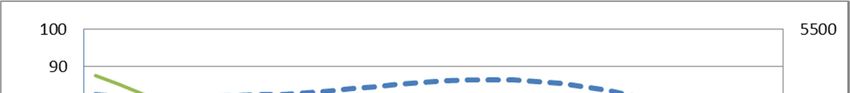
Much more important than the size of the expected interest savings is the insurance that the ERF
would provide, thereby shielding the euro area from sudden swings in market sentiments. While the
Fund is not a substitute for national fiscal discipline, it ensures that the results of the fiscal efforts
pursued by member countries are not wiped out by a disruptive confidence crisis.

The rest of the paper is structured as follows. Section 2 reviews previous proposals to introduce a
redemption fund for the European countries. In Section 3 we spell out the features of a
redistribution-free debt redemption scheme and study its financial implications. Section 4 discusses
various aspects of the moral hazard problem in connection with the functioning of the ERF. Section
5 concludes.

    2. Literature review

Since the start of the sovereign debt crisis, the introduction of an ERF has been proposed by several
authors (Table 2). Proposals differ in several ways, such as the size of the transferred debt, the time
horizon of the fund, the nature of the resources flowing from the member countries to the Fund, the
presence of ancillary provisions in order to rein in fiscal indiscipline.

The first detailed scheme was advanced by the German Council of Economic Experts (GCEE,
2011; see also Doluca et al. 2013). Participants would be allowed to refinance themselves through
the ERF up to a level equal to (or slightly higher than) the difference between the debt accumulated
to date and 60 per cent of GDP (the Maastricht reference value). This implies a transition phase
whose length depends on the schedule of the country-specific refinancing needs.8 Each country
would have to provide resources to the Fund yearly, of an amount sufficient to redeem the
transferred debt over a period of 20-25 years.9 This quick phase-out implies that, notwithstanding
the considerable reduction in sovereign yields on the remaining national debt that would be
achieved according to the proponents, participant countries would still be required to significantly
increase their primary balance. Each participating country would earmark a specific surcharge on a
national tax to guarantee its payments. Moreover, participants would pledge a sizeable amount of
resources (up to 20 per cent of the transferred debt) as collateral against their liabilities. In order to
avoid a new build-up of excessive imbalances, the GCEE requires the introduction of national fiscal
brakes, mandating a structural deficit below 0.5 per cent of GDP and residual national debt not

8
 Using January 1st 2012 as a fictitious starting date for the ERF, Doluca et al. (2013) estimate that the roll-in phase
would stretch over three to four years.
9
  Doluca et al. (2013) clarify how the annual payment has to be computed for each country. The first year, it is equal to
the EFR’s pro-rata annual interest payments plus one per cent of the amount of debt to be transferred. The country-
specific ratio between such an amount and nominal GDP in 2011 is then computed and used as a payment key in
proportion to/in relation to? GDP for the subsequent years. The hypotheses underlying the computation are a nominal
GDP growth rate of about 3 per cent and the ERF’s financing cost of 4 per cent.

                                                           7
exceeding 60 per cent. In the event that a country does not comply with its commitments, the roll-in
into the ERF is immediately halted, and the collateral lost for good.

Parello and Visco (2012) build upon the public debt redemption scheme proposed by the GCEE.
There are however two important differences: first, in their proposal the fund would operate for
slightly longer (around 30 years instead of 20-25); second, their ERF would only issue very long-
term bonds and, because of this, would record a surplus in the early years of operation. This initial
temporary surplus would be invested in low-risk financial instruments. While this time-profile of
the ERF’s outlays creates the possibility of investing on financial markets, it is not clear whether
this scheme is preferable overall to the plain vanilla GCEE approach. Indeed, the ERF would earn
more money on average, but its balance sheet would also become more risky, so markets might
require higher risk premiums on its bonds. The authors do not foresee any device to guarantee fiscal
discipline.

Another debt redemption scheme is outlined in Paris and Wyplosz (2014). Here, the scheme
involves the ECB buying sovereign bonds from each country in proportion to ECB capital keys, and
swapping them into zero-interest perpetuities (which is clearly tantamount to cancelling the debt).
The ensuing reduction in the ECB’s profits is passed on to governments via a reduction in
seigniorage revenues (again in proportion to ECB capital keys). In this way, each Member State
will pay the ECB back the total amount– in the present value sense – of the initial debt cancellation
in the form of reduced distributed profits over an indefinite future.

According to Paris and Wyplosz (2014), since both the national governments’ benefits (in terms of
initial debt cancellation) and losses are in proportion to the capital key, any explicit cross-country
transfer would be ruled out. The scheme is viable only as long as the ECB is able to generate a
sufficient stream of income over the infinite horizon without jeopardizing the achievement of its
inflation target. The authors argue that this is possible, providing simulations showing under what
combinations of interest rates, real growth and inflation, given the elasticity of money demand, the
present value of the future infinite stream of seigniorage is at least as big as the face value of the
cancelled debt. To deal with possible moral hazard, debt mutualization would be coupled with
stringent conditionality, embedded in a covenant. The authors specify that, should a country
accumulate debt again, the ECB would swap (part of) the zero-interest national perpetuities back
into interest-yielding bonds, thus deterring governments from sliding back into fiscal indiscipline.
Such a swap should be made automatic and linked to clearly specified trigger events. The role
assigned to the ECB by Paris and Wyplosz (2014) could also be played by another
intergovernmental body such as a reformed ESM, once all participating countries formally agree to
transfer a sufficient amount of their seigniorage to such an institution on a permanent basis.

Corsetti et al. (2015) suggest the launch of a one-off sovereign debt buyback by a stability fund,
financed through the commitment of future national revenues, sufficient to bring the debt of each
participating country below 95 per cent of GDP. The bonds thus acquired would then be swapped
into non-interest-bearing perpetuities. The fund would finance its purchases by issuing bills,
collateralized by dedicated future fiscal incomes − be it seigniorage, VAT or a wealth (transfer) tax

                                                  8
− of the participating countries over a long horizon (e.g. 50 years or more). The stability fund bills
would be accepted by the ECB in refinancing operations and could be bought by the ECB on the
secondary market in the event of liquidity shocks.
Table 1 Proposals for a debt redemption scheme
Size of the Time Resources paid to the Other enforcing tools
pooled tranche horizon ERF
German Council of debt exceeding 20-25 constant fraction of - strengthened national
Economic Experts 60% of GDP years GDP (mark-up on a fiscal rules
(2011) national tax, e.g. VAT - commitment to a medium-
and/or income tax) term consolidation and
growth strategy. If not
respected, ‘roll-in’
immediately discontinued
- pledge of collateral equal
to 20% of the loans
provided by the ERF. If
commitments are not
fulfilled, the collateral is
lost.
Parello and Visco debt exceeding 30 years
(2012) 60% of GDP
Paris and Wyplosz half of the infinite a fraction of - automatic call of
(2014) eurozone public horizon seigniorage revenues perpetuities back into
debt (distributed reimbursement in the
among countries event the remaining
on the basis of the national debt to GDP ratio
ECB capital keys) exceeds a given threshold
- national debt brakes
Corsetti et al. (2015) debt exceeding 50 years VAT, solidarity - introduction of an
90-95% of GDP surcharge, wealth tax automatic debt
or seigniorage restructuring mechanism
- regulatory changes that
limit the exposure of banks
to sovereign debt
The scheme could or could not envisage explicit between-countries redistribution. Corsetti et al.
(2015) start by proposing the calibration of a no-redistribution buyback scheme using only
seigniorage and VAT revenues. They first estimate the net present value of non-inflationary
seigniorage (i.e. compatible with an inflation target of 2 per cent) over a 50-year horizon,
considering a real interest rate ranging between 1 and 3 per cent, a real growth rate between 1 and 2
per cent and an elasticity of currency demand to output of 0.8 per cent. Depending on the
combination of parameters, the net present value of seigniorage ranges between €800 and €2,000
billion. If distributed according to the ECB capital keys, even in the more optimistic scenario, this
amount would not be enough to bring the debt-to-GDP level below 95 per cent for some countries
(namely Italy, Greece and Portugal). Such resources could be supplemented by additional VAT
revenues channelled directly into the stability fund. The authors estimate that VAT revenues equal
to 1 per cent of GDP in each country should be broadly sufficient to do the job. In order to use just
9the stream of income coming from seigniorage, it would be necessary to pool all resources together,
thus allowing for some redistribution among countries. The same is true in the event a solidarity tax
is adopted.
We should also mention a few other papers that, while they do not strictly speaking discuss
redemption funds, are relevant for our purposes as they outline forms of debt mutualization which
envisage country-specific repayments as a means to avoid cross-subsidization between core and
periphery countries (as we do in the present paper). In particular, Mayordomo et al. (2015) and
Minenna and Aversa (2018) suggest that national transfers should reflect each country’s CDS
premiums. According to Muellbauer (2013), transfers should instead be a function of a country’s
fiscal fundamentals.10 To our knowledge, the very short, informal note by De Grauwe and Moesen
(2009) is the only other contribution that suggests – as we do – that transfers should reflect the
sovereign yields prevailing at the start of the mutualization operation.
Finally, it should be noted that most proposals include provisions to ensure that each participant
honours its financial obligations to the Fund. This can be accomplished in a relatively
straightforward way by earmarking sources of revenue which can be credibly pledged by the States,
as is already the case with national contributions to the EU budget or to other international
organizations. While this potential source of moral hazard is easily addressed, a more difficult
problem concerns the effects of introducing the Fund on the participants’ incentives for fiscal
discipline in general (which we discuss in Section 4).
3. A redistribution-free European Redemption Fund
3.1 Overview
We propose that each euro-area country i transfers to the ERF at time 0 an amount of sovereign
bonds equal to a quota γ (the same for all participants) of its GDP:
= γY , ∀. 1
The transfer of national debt to the ERF is modelled as a one-off operation, ensuring an ideally
instantaneous redemption of the agreed fraction. We tend to prefer this solution as it would
minimize the risks of financial tensions which could arise in the transition phase, but is clearly not
the only way to implement the Fund: the analytic intuitions provided in this Section would be valid
overall also in the event of a more gradual phase-in.
10
Mayordomo et al. (2015) proposal is similar to that for “Esbies” in Brunnermaier et al. (2011). Minenna and Aversa
(2018) and Muellbauer (2018) aim at building a permanent common fiscal capacity, as an instrument to pursue an active
fiscal policy. In Muellbauer (2013), each country would be free to issue ‘Euro-insurance bonds’ in a decentralized way;
in Minenna and Aversa (2018), the issuance of the new bonds would be decided by a centralized entity.
10While the legal details of the scheme go beyond the scope of this paper, at a general level we could
envisage several alternative ways to implement such an instantaneous transfer.11 The first solution
would be for the ERF to buy the bonds on the market and simply scrap them, using the resources
provided by a large initial issuance of ERF bonds. A second solution consists in splitting each
existing bond into two distinct securities, one to be repaid by the Member State and one by the
ERF; the face value of the two bonds would reflect the share of national and supranational
responsibility respectively.12 What matters is that under both technical arrangements, part of the
national debts would be de facto transformed into ERF liabilities. Refinancing the transferred
fraction at maturity would become an exclusive responsibility of the ERF, and Member states
would be relieved from any direct debt-service obligation on the transferred fraction.
In exchange for this, member states would earmark yearly transfers to the ERF equal to a
percentage αi of their GDP:
= ∀, 2
These transfers would basically be used by the ERF to service and redeem its debt. We do not look
in detail at what national resources should be used to provide for the transfers. Transfers (such as
those for the EU structural funds) linked to a treaty obligation are usually considered safe.
However, earmarking a specific revenue source could be more credible.
What is crucial is that the fraction αi will be country-specific, reflecting the fact that countries differ
in their creditworthiness. Combining equations (1) and (2) makes it clear that the fraction can
be interpreted as the implicit interest rate charged by the ERF to the countries. In order to rule out
financial gains/losses from the scheme, we therefore require that for each participant this interest
rate be equal to the sovereign yield paid by the country before the launch of the ERF, which we call
ri :
= ∀ 3
In what follows, we will refer to eq. (3) as the no financial gain/losses condition.
For the ERF to be solvent, it must be the case that:
%
≡∑ ≤∑ ∑ & 1+ (4)
11
The accounting representation of the debt levels can differ as a consequence of the adopted legal solution. However,
the economics of the scheme and the related incentives do not change.
12
While the implementation of the first solution might be complex from the financial viewpoint (the mere
announcement of the operation might increase the market value of outstanding national debt overnight, making the
financing of the ERF more onerous while creating asymmetric capital gains for national states), the second solution
might be complex from a legal viewpoint, as it would constitute a unilateral contractual modification (the sovereign is
partly replaced by the ERF as debtor). A third option might be that the ERF unilaterally promises to pay pro-quota
interest and principal of each existing bond.
11That is, the future flow of transfers, discounted at the rate of interest at which the ERF is able to
borrow (rERF) should be equal to or higher than the initial level of debt. This is what we call the
solvency condition.
Given equation (1) and (2), after some algebra it turns out that this condition can be rewritten (under
the assumption of equal growth for all the countries) as:
≥( −* / 1+
where is the GDP-weighted average of the ,. The non-financial gain condition, together with
eq. 1, implies that:
=( ,
where r is the weighted average of the sovereign yields without the ERF. So, to the extent that:
≤ +* / 1− , (5)
the non-financial gain condition is sufficient for the solvency condition to hold.
Notice that condition (5) is a very conservative assumption, because it does not require that
≤ , which should instead realistically be the case, as the ERF should significantly reduce the
risk of a crisis in the euro area (risk which is instead included in the ris).
Other proposals (see for example Porello and Visco, 2012) have highlighted the further potential
gains which would stem from interest rate differentials between the current yields paid by the
sovereigns and those of an almost safe bond guaranteed by all member states. Of course the latter
would depend on the structure of the guarantees, which in turn determines the creditworthiness of
the ERF. It goes without saying that the creditworthiness (and therefore the benefits for high-debt
countries) would be higher with a structure of joint and unlimited guarantees (where all countries
are jointly responsible for the whole amount of the mutualized debt) rather than with limited
guarantees (where each country pledges an amount of collateral proportional to its transferred
debt).13 Whatever the structure of guarantees, exploiting gains from interest rates differentials is not
13
The provision of joint guarantees could be in conflict with the EU legal framework, if a strict interpretation of the no-
bail-out clause prevails. However, the evolution of the instruments and the conditions of financial assistance granted
during the sovereign debt crisis has shown that such a strict interpretation has been de facto overcome. In particular, in
2011 an amendment to Article 136 of the Treaty on the Functioning of the European Union has been introduced by
inserting the following text: ‘The Member States whose currency is the euro may establish a stability mechanism
to be activated if indispensable to safeguard the stability of the euro area as a whole. The granting of any required
financial assistance under the mechanism will be made subject to strict conditionality'. This amendment paved the way
for setting up the ESM and could, in principle, provide the legal basis to authorize countries to pledge joint and
unlimited guarantees to the ERF.
12the focus of our proposal. Such gains are difficult to identify ex ante: therefore, in our baseline
simulation we prefer to be on the safe side and we set the size of the yearly transfer to the ERF on
the basis of prudent assumptions of interest rates and growth.14
In general, the solvency condition does not guarantee that the ERF’s debt goes down over time, i.e.
that the annual inflows from participating countries are more than sufficient to cover the ERF’s
interest bill and the debt that comes due. However, we will show that realistic assumptions for
interest rates and growth and a proper calibration of the transfers do ensure that the ERF is not
systematically in deficit and that mutualized debt is fully repaid in a finite time even if, differently
from previous proposals (Corsetti et al., 2015; Doluca et al., 2013; Parello and Visco, 2012), the
deadline to fully redeem ERF’s debt is not fixed ex ante. In our proposal, the length of the
redemption phase is endogenous and it depends on two parameters: the prevailing interest-growth
differential and the size of the annual payments received from the countries. The fact that the length
of the debt redemption phase is not fixed ex ante allows some counter-cyclicality within the
repayment scheme: during recessions the payment to the ERF decreases in nominal value, thus
lowering the effort required for a country to be compliant with the scheme commitments and
therefore enhancing its credibility.
Finally, it should be acknowledged that, no matter how realistic the assumptions and accurate the
calibrations, in the real world the implementation of the scheme may lead to some financial
redistribution ex post. This would be the case, for example, if the macroeconomic assumptions on
which payments are calibrated turned out to be wrong. To address this issue, the ERF’s design (in
terms of countries’ annual payment, penalizations and allowances) should be periodically revised to
adapt to changing macroeconomic conditions and/or to compensate for outturns different from the
forecasts used for the original design. The frequency of the revision must take account of long-term
structural trends rather than business cycle-related economic fluctuations (for example, a revision
every 8-10 years could be appropriate).
3.2 Baseline calibration
Numerical examples can be used to show how the scheme outlined in general terms in the previous
section would work in practice. For this purpose, two scenarios are compared: one with no policy
changes (No-ERF baseline scenario) and the other featuring the introduction of the ERF (ERF-
baseline scenario).
As a first step, we constructed the baseline scenario without the ERF for the debt dynamics in the
four largest euro-area countries (Germany, France, Italy and Spain)15 based on realistic assumptions
14
In the simulations below we assume that all countries have the same rate of potential growth. However, in principle,
the annual payment is to be modulated to take into account structural differentials in economic growth across countries.
If a Member State permanently grows less than its partners, it can be required to increase its annual contribution to the
scheme (in terms of incidence over its GDP) in order to avoid free- riding on the growth dividends of other countries.
13about growth and interest rates. For the years 2017-18 we used the 2017 Autumn European
Commission economic forecasts for each country. Starting from 2019, we assumed the following:
• the primary balance is set to gradually increase (by 0.5 percentage points of GDP yearly, in
line with the general requirements of the preventive arm of the Stability and Growth Pact -
SGP)16 until reaching the budget balance which is maintained thereafter;
• countries’ interest expenditure reflects the average interest rate paid on the existing stock of
debt, the interest rates at issuance and the maturity structure as of the first quarter of 2018; it
is computed considering the effects (common for all the participating countries) of a gradual
increase (from 2019 to 2025) of the ECB monetary policy reference rates;
• all economies are assumed to grow at a yearly rate of 3.5 per cent starting from 2019, which
reflects a real GDP growth of 1.5 per cent and a GDP deflator in line with the ECB inflation
target.
Figure 1 shows the projected dynamics of the average cost of debt in the four countries. The
differences in 2018 reflect the differential impact that the sovereign debt crisis had on the four
countries. Values range from 2.7 per cent in Italy to 1.7 per cent in Germany. The gap at the end of
the projection horizon only mirrors the currently observed differentials among the interest rates at
issuance (monetary policy affects all countries’ interest spending in the same way).
Figure 1. Projected average cost of debt (2018-2048)
Source: our calculations taking into account current rates at issuance, maturity structure of debt and
assuming a gradual increase of the MRO by 3 percentage points over seven years (2019-2025)
The dispersion in the individual countries’ average interest rate at the end of the simulation period
halves with respect to the start of the period: this reflects the rather uniform (they are all close to
15
We only considered these four countries, with no loss of generality, to keep the presentation of the scheme as simple
as possible. Of course the building blocks of our simulations remain valid and can be adapted to extend the scheme to
all the euro-area Member States.
16
The requirement in terms of fiscal effort can be made country-specific by taking into account the individual cyclical
conditions.
14zero) interest rates currently charged at issuance to euro-area countries (that gradually affect the
stock of sovereign debt according to the maturity structure).
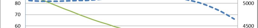
Figure 2 (blue bars) shows the debt dynamics in each country in the No-ERF baseline scenario.
Under the assumption that countries’ primary balances comply with the SGP and point towards a
balanced budget, public debt is expected to fall significantly over the next 30 years in all countries,
also benefiting from a favourable interest-growth differential over the next 5 years.
Figure 2. Projected baseline national debt-to-GDP ratio dynamics with and without the ERF
(2018-2048)
IT DE
140.0 140.0
120.0 No-ERF baseline 120.0
No-ERF baseline
ERF baseline ERF baseline
100.0 100.0
80.0 80.0
60.0 60.0
40.0 40.0
20.0 20.0
0.0 0.0
FR ES
140.0 140.0
120.0 120.0 No-ERF baseline
No-ERF baseline
100.0 ERF baseline 100.0
ERF baseline
80.0 80.0
60.0 60.0
40.0 40.0
20.0 20.0
0.0 0.0
Note: in the ERF scenario the national debt is the quota of sovereign debt not transferred to the ERF which
has to be refinanced by each individual country.
Clearly, the debt level in Italy remains rather high for some years to come and only goes below 100
per cent of GDP in 2027. This notwithstanding, Italy records a 30- percentage- point reduction in
around ten years, whereas France and Spain would bring their debt down by 20 percentage points
(to below 80 per cent) over the same time span.
As a second step, we constructed the ERF-baseline scenario in which a redemption scheme is
introduced. At the end of 2018, the participating countries transfer an amount of debt (what we
labeled γ in the previous Section) to the ERF, equal (for the sake of exposition) to 60 per cent of
their own GDP via a one-off operation. This quota represents the benchmark; the actual share of
transferred debt varies according to the current incidence of public debt in each country. Countries
with a current debt above 120 per cent of GDP should be allowed to transfer more (even though at
the cost of a penalization; see below), while virtuous countries already compliant with the
Maastricht threshold would transfer less debt and would thus benefit from a more favourable
15treatment (see below). In the case of Italy, whose debt exceeds 130 per cent of GDP, a transfer of 60
per cent of its GDP would not suffice to bring the national debt below the Maastricht threshold.
Therefore Italy would transfer a higher share of debt, namely 70 per cent of GDP so as to end up
with a national debt level below the threshold. At the other extreme, Germany, whose public debt is
around the threshold, would transfer a lower quota, for example 50 per cent of GDP. The
redemption mechanism would start operating in 2019.
Another possibility would be to leave each participant free to transfer an amount of debt between a
minimum and a maximum, expressed as percentages of national GDP. We think that, while in
principle thresholds are not necessary, it is important that each country puts a significant stake in
the ERF project, as a means of effectively communicating its commitment to the success of the
project itself and, more broadly, to the EMU endeavour.
Obviously, introducing the ERF requires making further assumptions on many different parameters
of the scheme. They are set in such a way as to minimize cross-country transfers. As discussed
above, the yearly payment from countries, set equal to a fixed percentage (αi) of national GDP, is
meant to finance the redemption of the debt transferred to the ERF by the individual countries. In
the benchmark case, for most countries αi equals 1.2 per cent of their GDP, which represents an
implicit interest rate ( /( of around 2 per cent on the transferred tranche of debt (60 per cent of
GDP).17 For countries with low public debt, an allowance of around 0.2 percentage points is
provided: the annual transfer is lowered to around 1 per cent of GDP per year to keep the implicit
interest rate equal to the one that is paid by the other countries. For high-debt countries, the transfer
is increased by a penalization of around 0.5 percentage points of GDP. As a result, the implicit
interest rate on their transferred debt is around half a percentage point higher.
The interest rate paid by the ERF on its debt, is initially equal to the weighted average of the
interest rates paid by governments on their sovereign debts, as its debt fully reflects the current
maturity structure of national public debts. In order to project the future evolution of ERF debt, we
also require an assumption for the interest rate paid by the ERF on the new debt issued to roll over
the expiring bonds. This parameter signals the market’s assessment of the ERF’s riskiness and it is
crucial because it shapes the countries’ interest rate differential between the mutualized and the
national tranche of their sovereign debt and is therefore the main driver of financial gains or losses
for both the ERF and individual countries. We acknowledge that making forecasts for this
parameter is very difficult. In the baseline we set such a rate as being equal to the weighted average
currently observed for national governments and we assume that it will increase following the
pattern of monetary policy reference rates. Let us remark again that this is a very conservative
17
The size of national payments is kept fixed, although the ERF’s debt is gradually redeemed. Since the country’s pro-
quota mutualized debt decreases through the simulation horizon, this is equivalent to setting a gradually increasing
implicit interest rate on the national quota.
16assumption, as it rules out any benefit stemming from the elimination of a tail risk of a sovereign
crisis and also any discount stemming from the high liquidity of the ERF bond.
The red bars in Figure 2 show the dynamics of national debts placed on the market in the ERF-
baseline scenario.18 By assumption, the introduction of the redemption scheme mechanically
reduces the ratio of national debt to national GDP in the first year of simulation (2018); in the
projection horizon this ratio continues to decline, even though at a slower pace compared with the
baseline scenario without the ERF.
In order to quantify the financial effects of the introduction of the ERF, we focus on two metrics,
for countries and for the ERF respectively, both expressed in terms of the net present value (NPV)
over the first ten years of the simulation horizon (2019-2018).
The metric used for countries is the NPV of the difference in interest expenditure between the ERF
baseline and the No-ERF baseline scenario, both discounted by a discount rate R, as follows:
9: 7 6 97
5 = ∑8./ 7
4
- ∑8./ 7
/6 /6
In this formula, rit and r’it are country i’s sovereign yields before and after the introduction of the
ERF. As discussed in Section 3.1, if the αi that we have chosen in our calibration is close to those
that would guarantee the no loss/gains condition, Ait should be close to zero, independently of the
discount rate. In other words, the yearly total interest expenditure should be the same in both
scenarios.
The metric used for the ERF is the NPV of its budget balances over the same period, where the
single period balances are given by:
0 , =∑-./ - 123,4 123,4−1 ∀4
i.e. they are given by the difference between the interest (rERF) paid on the ERF’s debt and the sum
of the annual payments (∑-./ ) received by all countries.19
The overall gain/loss over the chosen time horizon is simply given by:
0123,4
∑-./ 5 - ∑8./ 7
/6
All the metrics above are normalized by the 2019 GDP (national GDP for individual countries and
the total GDP for the ERF). For the discount rate we have chosen rERF. Table 2 displays the results
for the baseline scenario in terms of NPV over the years 2019-28: the neutrality of the calibration is
18
The drop in national debt in 2019 reflects the drop in the share of debt to be refinanced by each country. The
statistical treatment of the transferred share is uncertain, as it could be recorded either as national debt (as in the EFSF
case), or as the debt of a supranational institution (as in the case of the ESM). In our simulations, we stick to the second
interpretation.
19
The solvency condition ensures that the sum of the yearly ERF balances is positive and is large enough to repay the
initial ERF debt over an infinite horizon, but this is not guaranteed over a finite horizon.
17confirmed by the very small size of the financial effects for each country stemming from the
scheme. The change in interest spending is broadly nil for Germany, France and Italy.
Table 2. Gains (+) / Losses (-) in the baseline-neutral scenario(*) (as % GDP)
ERF-baseline versus No-ERF baseline
Italy Germany France Spain ERF (surplus) Total
0.0 0.1 -0.1 1.0 0.0 0.1
(*) Gains/losses are expressed as the NPV over the years 2019-2028 of the difference in interest spending between the
ERF-baseline and the No-ERF baseline scenarios for the Member States, normalized by their respective 2019 GDP; ii)
the budget balance for ERF, normalized by the total GDP for 2019 (computed by summing the GDPs of the
participating countries).
The gain for Spain comes from a technical issue with the parametrization strategy: Spain and
France have a similar debt level and, as such, according to our scheme, they are treated equally in
terms of required annual payment and of transferred debt (. Nevertheless, they have a
significantly different initial average cost of debt (higher in Spain, as shown in Figure 1); therefore
their gains cannot be brought down to zero simultaneously.20 While Italy has an average cost of
debt similar to that of Spain, it transfers a higher share of debt and the penalization can be set so as
to bring its gain to zero.
The neutral calibration of the redemption scheme in the baseline scenario ensures a broadly
balanced ERF budget and a steady decline of the ERF’s debt as a share of total GDP (Figure 3).
Figure 3. Projected dynamics of debt-to-GDP ratio in an ERF-baseline scenario (2018-2048)
20
Alternatively, we could have set the parameters in such a way as to shift down to zero and to a loss the financial
effects respectively for Spain and for France. The calibration can also be made more detailed by modulating the annual
payments also on the basis of the average interest rate paid on national debt.
18Starting at around 60 per cent of total GDP, ERF debt goes down to around 40 per cent in 10 years
and below 30 per cent of total GDP in 20 years (reaching zero in 2065). In nominal terms the ERF’s
debt remains close to its starting value for around 20 years; 21 it starts declining afterwards. The
total debt of the area, given by the sum of the ERF’s and the national tranches of public debt would
steadily decrease from around 90 per cent of total GDP to around 30 per cent at the end of the 30-
year simulation period. This dynamic is very similar to how the total debt would evolve in the
baseline scenario without the ERF.
We have shown, therefore, that it is possible to design a redemption scheme that minimizes induced
financial effects with respect to the No-ERF baseline scenario.
Given that the dynamics of the total debt of the area are not significantly affected, and that national
debt dynamics are mostly driven by the evolution of primary balances, we might ask what
difference the scheme makes. However, this critique misses two crucial points. First, the
quantitatively small benefits are due to the very conservative hypotheses that we have made
concerning the post-ERF evolution of the interest rates. Second, and more importantly, the primary
aim of the ERF is to shield the euro area from the risk that sudden swings in market sentiment
trigger a liquidity crisis in one or more high-debt member states and therefore area-wide financial
turmoil. This reduction in uncertainty is a highly valuable good in itself (and would ultimately be
translated into lower risk premiums).
3.3 Sensitivity analyses
As we have seen, using our baseline calibration, cross-country subsidization is negligible. It could
be argued that this feature is heavily dependent on such a calibration. In this section we test the
robustness of this result based on alternative, though plausible, assumptions concerning (i)
economic growth rates (both in ERF and No-ERF baseline scenarios); (ii) the yield required by the
market on the ERF’s newly-issued debt; and (iii) the interest rate of the remaining national debt
after the introduction of the ERF.
The financial effects of the ERF in the scenario based on alternative growth assumption are shown
in Table 3. In column (2) it is assumed that, starting from 2019 the average nominal GDP growth
rate is permanently reduced by half a percentage point (to 3 per cent) in each country (and therefore
in the area as a whole); in column (3) such a reduction in growth is assumed to occur only in Italy.
21
The debt peaks in 2036, but the increase is marginal: a 2 per cent increase over 18 years.
19Table 3. Gains (+) / Losses (-) in the alternative growth scenarios(*)
4 (as % GDP)
Baseline Lower growth Lower growth
(-0.5%) only in Italy
(1) (2) (3)
Italy 0.0 0.5 0.5
Germany 0.1 0.3 0.1
France -0.1 0.2 -0.1
Spain 1.0 1.3 1.0
ERF (surplus) 0.0 -0.4 -0.1
Total 0.1 0.1 0.1
(*) Gains/losses are expressed as the NPV over the years 2019-2028 of the difference in
interest spending between the ERF-baseline and the No-ERF baseline scenarios for the
Member States, normalized by their respective 2019 GDP; ii) the budget balance for ERF,
normalized by the total GDP for 2019 (computed by summing the GDPs of the
participating countries).
With lower growth, the introduction of the ERF provides some gains to the countries concerned. In
fact, in nominal terms the interest bill on the national tranche would be unchanged but the annual
transfer to the ERF would be lower; the combined effect would determine a lower NPV for the total
future interest expenditure. This feature of the scheme provides some degree of counter-cyclicality
in the debt reduction plan. For the same reasons, the ERF would run annual deficits in some years.
In the event that all countries grow at a slower pace ERF would therefore register a loss of almost
half a percentage point of total GDP (in NPV terms) over 10 years. Yet the loss is of a limited
magnitude and in order to be redressed (and therefore to downsize the gains for countries) it would
be enough to slightly increase (by less than 0.1 percentage points of GDP) the countries’ annual
transfers, with limited impact on their implicit interest rate. Under the assumption that only Italy
grows less than its partners structurally speaking, it would be enough to marginally increase its
annual payment to the Fund to minimize the financial effects.
Figure 4 compares the debt dynamics of the ERF and of participating countries when growth is set
at 3.5 per cent (left-hand panel) and at 3.0 per cent (right-hand panel) for all members. Obviously,
in the latter scenario the reduction of the incidence of debt on GDP would be slower22 both for
countries and for the ERF (at the end of the period it would attain 25 per cent of total GDP, around
5 percentage points higher than in the baseline scenario) and the ERF’s debt in nominal terms
would not decrease.
22
This result is due both to a denominator effect, since the product is smaller, and to an increase of the numerator
driven by a higher interest bill paid on the public debt that is reducing at a slower pace.
20Figure 4. Debt-to-GDP ratio dynamics: ERF baseline (left) and Lower growth (right)
scenario
However, the pattern of ERF debt may be changed and brought to the previous declining one by
simply raising the annual payment from countries to the Fund by around 0.1 percentage point of
GDP. Should only Italy grow at a slower pace, at the end of the decade the ERF’s debt would only
be one point higher than in the baseline scenario.
Alternative assumptions on the interest rate paid by the ERF on its new debt issuances are shown in
Table 4. This parameter is important because it determines the payoff of the scheme both for the
participating countries and the ERF, and it is very difficult to forecast. In fact, the price at issuance
of the ERF’s debt will be determined by both the institutional characteristics of the scheme (e.g. the
guarantee structure) and the perceived future riskiness of the participating countries and of the area
as a whole. In our baseline scenario we assumed that the interest rate on the new ERF bond equals
the weighted average of the current rate for the participating countries.
Table 4. Gains (+) / Losses (-) in the alternative interest rate scenarios(*) (as % GDP)
ERF-Baseline ERF interest ERF interest rate ERF avg. interest
rate as Italy rate down (1%)
as Germany
(1) (2) (3) (4)
Italy 0.0 0.0 0.0 0.0
Germany 0.1 0.1 0.1 0.1
France -0.1 -0.1 -0.1 -0.1
Spain 1.0 1.0 1.0 1.0
ERF (surplus) 0.0 0.3 -1.0 5.0
Total 0.1 0.5 -0.8 5.2
(*) Gains/losses are expressed as the NPV over the years 2019-2028 of: the difference in interest spending between
the ERF-baseline and the No-ERF baseline scenarios for the Member States, normalized by their respective 2019
GDP; ii) the budget balance for ERF, normalized by the total GDP for 2019 (computed by summing the GDPs of
the participating countries).
21It could be assumed instead that this interest rate will converge toward the issuance rate of
Germany, the lowest value among the participating countries (this might be the case if markets
believe that the introduction of the ERF effectively eliminates the risk of sovereign liquidity crises
and of any related systemic instability in the area). At the other extreme, as argued in Balassone et
al. (2016), the interest rate might converge to that paid on Italian bonds, i.e. ‘to that of the bonds
issued by the riskier countries in the pool with a debt large enough to damage the creditworthiness
of the least risky countries’. In both cases, if the interest rate at issuance of the national tranches is
unchanged, all participating countries are as well off as in the baseline scenario.
As for the Fund, in the former case it would benefit from a slightly lower interest expenditure and it
would run a small cumulative surplus of 0.3 percentage points of total GDP over the next ten years
(in NPV terms), as shown in Column (2). This scenario would be marginally more favourable than
the baseline one; it would need no adjustment in parameter calibration to ensure its neutrality and it
would determine a more sizeable reduction of mutualized public debt both in nominal terms (Figure
5, left vertical axis) and as a share of the total GDP (Figure 5, right vertical axis).
5
Figure 5. Dynamics of the ERF’s debt under alternative hypotheses on the issuance rate
5600 60.0
5400 55.0
50.0
5200
45.0
5000
40.0
4800
35.0
4600
30.0
baseline nominal ERF as DE nominal
4400
25.0
ERF as IT nominal baseline % GDP
4200 20.0
ERF as DE % GDP ERF as IT % GDP
4000 15.0
If, on the contrary, the ERF’s issuance rate is in line with the Italian one (Table 3, Column 3), the
ERF will run a cumulative deficit of about 1 percentage point of total GDP (0.1 percentage points
per year), while the financial effects for participating countries remain close to zero (with Spain as
an exception), as in the baseline. This would be a ‘pessimistic’ baseline scenario, with a less marked
decrease in the incidence of the mutualized public debt (see again Figure 5).23 However, in order to
improve the neutrality of such a scenario and to equalize the financial effects for the participating
countries and for the ERF it would be enough to marginally increase the parameter α for annual
payment from all countries: in this way the cumulative deficit for the ERF would be halved over the
next decade (to around 0.5 percentage points of total GDP) and the cumulative loss of the country
would be about the same size (in terms of their respective GDP, with the exception of Spain).
23
Mutualized debt would increase in nominal terms (Figure 5, left vertical axis).
22As a final exercise, in Table 5 we study what would happen if markets reacted to the introduction of
the ERF by changing the risk premiums required on the remaining national public debt (the interest
rates required in the No-ERF baseline scenario are unchanged). Column (2) shows the effects of a
Countries up (+1%) scenario: over the first ten years of the simulation (2019-28) the average
interest rate on the national part of the debt (with the exception of Germany) is increased by 100
basis points, while the interest rate of the ERF is unchanged with respect to the baseline scenario.
This scenario can be rationalized through an adverse market perception of the national tranches
(perceived as riskier) due to: (i) the reduced liquidity of these assets; and (ii) a higher risk of default
stemming from the fact that the no bail-out clause might appear more credible (because national
debts no longer pose systemic threats). The Countries-up scenario would have some heterogeneous
financial effects: Italy would suffer the most, due to the still high tranche of national debt.
Compared with the baseline scenario with ERF, the loss for France is only slightly higher than for
Spain. The total area loss (compared with the ERF baseline) in NPV terms over the next ten years
would equal 2.5 percentage points in cumulative terms (around 0.25 percentage points per year).
Therefore, the overall effect of a change of 100 basis points on the average interest rate of national
debts is about half the impact of a change of the same proportion in the ERF’s debts. The dynamic
of national public debt would remain unchanged under the assumption that any increase in the
interest bill is compensated by an increase of the primary balance in line with the SGP until a
balanced budget is reached.24
Table 5. Gains (+) / Losses (-) in scenarios with market reactions to the introduction of the
ERF (as % GDP)
ERF-Baseline Countries up (+1%) ERF down (1%) +
Countries up (1%)
(1) (2) (3)
Italy 0.0 -5.2 -5.2
Germany 0.1 0.1 0.1
France -0.1 -4.2 -4.2
Spain 1.0 -2.5 -2.5
ERF (surplus) 0.0 0.0 5.0
Total 0.1 -2.5 2.5
(*) Gains/losses are expressed as the NPV over the years 2019-2028 of: the difference in
interest spending between the ERF-baseline and the No-ERF baseline scenarios for the
Member States, normalized by their respective 2019 GDP; ii) the budget balance for the
ERF, normalized by the total GDP for 2019 (computed by summing the GDPs of the
participating countries).
Column (3) shows the effects of an ERF down (-1%) and countries up (+1%) scenario: over the first
ten years the average interest rate on ERF debt is reduced by 100 basis points while that of the
24
Should a country not compensate the higher interest spending by means of higher primary surpluses, the reduction of
national debts would be slowed down.
23You can also read