Asymmetric Macroeconomic Effects of QE-Induced Increases in Excess Reserves in a Monetary Union - Maximilian Horst Ulrike Neyer Daniel Stempel ...
←
→
Page content transcription
If your browser does not render page correctly, please read the page content below
NO 346

Asymmetric Macroeconomic Effects of
QE-Induced Increases in Excess Reserves
in a Monetary Union
Maximilian Horst
Ulrike Neyer
Daniel Stempel

July 2020
IMPRINT

D IC E D I SCU SSI ON PAP E R

Published by:
Heinrich-Heine-University Düsseldorf,
Düsseldorf Institute for Competition Economics (DICE),
Universitätsstraße 1, 40225 Düsseldorf, Germany
www.dice.hhu.de

Editor:
Prof. Dr. Hans-Theo Normann
Düsseldorf Institute for Competition Economics (DICE)
Tel +49 (0) 211-81-15125, E-Mail normann@dice.hhu.de

All rights reserved. Düsseldorf, Germany 2020.

ISSN 2190-9938 (online) / ISBN 978-3-86304-345-2

The working papers published in the series constitute work in
progress circulated to stimulate discussion and critical comments.
Views expressed represent exclusively the authors’ own opinions
and do not necessarily reflect those of the editor.
Asymmetric Macroeconomic Effects of QE-Induced Increases
in Excess Reserves in a Monetary Union
Maximilian Horst* Ulrike Neyer Daniel Stempel
July 2020
Abstract
The Eurosystem’s large-scale asset purchases (quantitative easing, QE) induce a strong
and persistent increase in excess reserves in the euro area banking sector. These excess
reserves are heterogeneously distributed across euro area countries. This paper develops
a two-country New Keynesian model – calibrated to represent a high- and a low-liquidity
euro area member – to analyze the macroeconomic effects of (QE-induced) heterogeneous
increases in excess reserves and deposits in a monetary union. QE triggers economic
activity and increases the union-wide consumer price level after a negative preference
shock. However, its efficacy is dampened by a reverse bank lending channel that weakens
the interest rate channel of QE. These dampening effects are higher in the high-liquidity
country. We find similar results in response to a monetary policy shock. Furthermore, we
show that a shock in the form of a deposit shift between the two countries, interpreted
as capital flight, has negative (positive) effects for the economy of the country receiving
(losing) the deposits.
JEL classification: E51, E52, E58, F41, F45.
Keywords: unconventional monetary policy, quantitative easing (QE), monetary policy
transmission, excess liquidity, credit lending, heterogeneous monetary union, New Keyne-
sian model.
*
Heinrich Heine University Düsseldorf, Department of Economics, Universitätsstraße 1, 40225 Düssel-
dorf, Germany, phone: +49-211-81-15342, email: maximilian.horst@hhu.de.
Heinrich Heine University Düsseldorf, Department of Economics, Universitätsstraße 1, 40225 Düssel-
dorf, Germany, email: ulrike.neyer@hhu.de.
Heinrich Heine University Düsseldorf, Department of Economics, Universitätsstraße 1, 40225 Düssel-
dorf, Germany, email: daniel.stempel@hhu.de.
1       Introduction

In January 2015, the Eurosystem1 launched its large-scale asset purchase program, often

referred to as quantitative easing (QE), to address the risks of too low, temporarily even

negative, inflation rates for a too prolonged period. The objective of this program is to

directly lower long-term interest rates at times when (short-term) monetary policy interest

rates are approaching the effective lower bound, so that it is no longer possible to realize

expansionary monetary policy impulses by conventionally decreasing short-term interest

rates.2 When implementing QE in the euro area, the intent is for aggregate demand, and

hence the price level, to increase until the target inflation rate of below, but close to, 2%

over the medium-term is reached (European Central Bank, 2015). As a consequence of the

Eurosystem’s QE program, excess reserves in the euro area banking sector have increased

to unprecedented levels.3 However, the way QE is implemented in the euro area implies

that these excess reserves are not homogeneously distributed across euro area countries.

    Against this background, we develop a two-country New Keynesian model to analyze

the macroeconomic effects of (QE-induced) heterogeneous increases in excess reserves and

deposits in a monetary union (i.e., whether or not heterogeneously distributed excess re-

serves and deposits are just a technical feature without “real effects”). In our model,

QE is the monetary policy tool. We conceptualize positive net asset purchases by the

central bank to have two effects. First, they decrease the relevant interest rate for house-

holds’ consumption and firms’ investment decisions. Second, they imply an increase in the

banking sector’s excess reserve and deposit holdings, leading to increasing balance sheet

costs for banks. We calibrate the model to represent a high- and a low-liquidity euro
    1
       The term “Eurosystem” includes the institutions responsible for monetary policy in the euro area,
i.e., the European Central Bank (ECB) and all euro area national central banks (NCBs). For simplicity,
we use the terms ECB and Eurosystem synonymously in this paper.
     2
       Note that in January 2015 the interest rate on the ECB’s main refinancing operations (MROs) already
amounted to .05%, the interest rate on its deposit facility was already negative at -.2%, and the interest
rate on the marginal lending facility was at .3% (data source: ECB).
     3
       Excess reserves are here defined as the sum of (i) commercial banks’ current account balances at their
national central bank in excess of those contributing to minimum reserve requirements, and (ii) deposits
held at the ECB’s overnight deposit facility. In ECB parlance this quantity is defined as “excess liquidity”
since the ECB uses the term “excess reserves” to define the narrower concept of current account balances
in excess of reserve requirements. We refer to excess reserves as all central bank overnight deposits beyond
required reserves and hence do not distinguish between whether they are held on a current account or at
the deposit facility. Since June 2014 excess reserves have been remunerated at a negative rate, currently
(June 2020) at -.5%. Neglecting the recently (December 2019) introduced “two-tier system”, this interest
rate has to be paid independently of whether the liquidity is held in the ECB’s overnight deposit facility
or on current accounts with the Eurosystem (European Central Bank, 2019).

                                                     1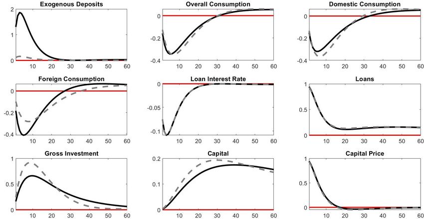
area country (Germany and Italy). Thus, in steady state, excess reserves and deposits are

already asymmetrically distributed between the two countries. Considering the specific

implementation of QE in the euro area that reinforces this heterogeneous liquidity dis-

tribution, allows us to identify two transmission channels of QE: an interest rate channel

and a reverse bank lending channel.

   We analyze the model responses to three shocks: a preference shock, a shock in the form

of a deposit shift between the two countries (deposit shift shock), and a monetary policy

shock. We find that after a symmetric, negative preference shock (implying a decrease in

household consumption) in both countries, the stabilizing effects of expansionary monetary

policy are weakened due to the implied increases in excess reserves and deposits. The

central bank reacts to the shock-induced decreasing union-wide inflation with positive net

asset purchases. This expansionary monetary policy measure leads to a decreasing interest

rate and increasing excess reserves and deposits. The decreasing interest rate triggers

economic activity and thus increases union-wide consumer price inflation. However, the

increasing excess reserves and deposits weaken these effects (increasing balance sheet costs

for banks due to increased deposits imply a dampening effect on lending), i.e., the interest

rate channel of QE is dampened by a reverse bank lending channel. These weakening

effects are more pronounced in the high-liquidity country.

   The deposit shift shock implies that deposits and thus (excess) reserves are moved

from the low-liquidity country to the high-liquidity country, which can be interpreted as

capital flight (“safe-haven-flows” or “flight-to-quality” phenomena), for instance. This

increase in deposits and excess reserves leads to higher balance sheet costs for banks in

the high-liquidity country. Consequently, in that country, economic activity decreases.

Analogously, the low-liquidity country benefits from the deposit shift.

   The monetary policy shock in the form of an unexpected increase in the central bank’s

net asset purchases, implies an initial decrease in the real interest rate and an initial

increase in excess reserves and deposits. Again, the stabilizing effects of the monetary

policy reaction to this shock are dampened by the costs associated with excess reserves,

i.e., the reverse bank lending channel weakens the interest rate channel of QE. These

dampening effects are larger in the high-liquidity country.

                                             2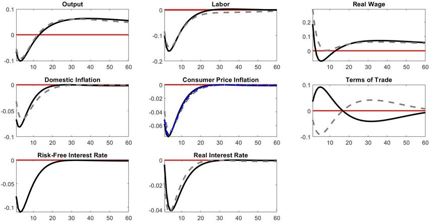
Our paper primarily builds on three strands of literature. First, we contribute to

the literature on DSGE models that include a banking sector to analyze the effects of

unconventional monetary policy measures, such as QE. Respective examples are Gerali

et al. (2010), Cúrdia and Woodford (2011), Gertler and Karadi (2011, 2013), Chen et al.

(2012), Brunnermeier and Koby (2018), Kumhof and Wang (2019), and Wu and Zhang

(2019a,b). Note that as in Jakab and Kumhof (2019) and Kumhof and Wang (2019), we

assume that banks create deposits endogenously by granting loans (i.e., banks provide

“financing through deposit creation”). Second, our work is related to several papers that

develop DSGE models to analyze monetary policy effects in a monetary union such as

in Benigno (2004), Beetsma and Jensen (2005), Galı́ and Monacelli (2005, 2008), Ferrero

(2009), Bhattarai et al. (2015), and Saraceno and Tamborini (2020). Third, our work is

based on literature investigating the relationship between the implementation of QE and

the creation of excess reserves. Examples include Alvarez et al. (2017), Baldo et al. (2017)

and Keister and McAndrews (2019).

   Our paper contributes to these strands by combining empirical evidence on the tech-

nical particularities of the implementation of QE by the Eurosystem, including the effects

on excess reserves, with a realistically calibrated New Keynesian model of the euro area.

To the best of our knowledge, our paper is the first one to endogenously implement the de-

velopment of excess reserves accompanying QE and to analyze the macroeconomic effects

of this mechanical relationship in a monetary union model.

   The remainder of this paper is organized as follows. Section 2 presents some notable

fundamentals with regard to the implementation of QE in the euro area. In Section 3,

we develop the model and derive the corresponding equilibrium. Section 4 describes the

model calibration and derives and analyzes the results with regard to three different shocks.

Section 5 concludes.

                                             3
2 A Note on the Implementation of Quantitative Easing in
the Euro Area
The ECB’s large-scale asset purchase program (APP), commonly referred to as QE, in-
volves four programs under which both private and public sector securities are purchased.4
As a consequence of the implementation of QE, aggregate excess reserves5 in the euro area
increased from 200 billion euros in March 2015 to a record high of 1.9 trillion euros in
December 2018.6 The excess reserves are asymmetrically distributed across euro area
countries. Since the beginning of QE, about 30% of overall excess reserves are, for exam-
ple, held solely in Germany (see Figure 1). Alvarez et al. (2017) and Baldo et al. (2017)
show that approximately 80-90% of total excess reserves predominantly accumulate in
Germany, the Netherlands, France, Finland, and Luxembourg, whereas such holdings are
much less pronounced in Italy, Portugal or Spain, for example.
Note that both an increase in excess reserves as well as a very similar heterogeneous
distribution of this liquidity among euro area countries could already be observed during
the financial and sovereign debt crisis (see Figure 1). However, compared to the QE
period the reason for the heterogeneous distribution during these periods was different. In
particular, capital flight (so-called “safe-haven-flows” and “flight-to-quality” phenomena)
from lower-rated to higher-rated euro area countries was the main provoking factor at that
time (Baldo et al., 2017).
By implementing QE, each euro area national central bank purchases assets according
to its share in the ECB’s capital key, inter alia, domestic government bonds. The asset
purchases are funded through the creation of reserves by the Eurosystem, implying that
total excess reserves in the banking sector mechanically increase. As a consequence of
4
The APP consists of the Corporate Sector Purchase Programme (CSPP), the Public Sector Purchase
Programme (PSPP), the Asset-Backed Securities Purchase Programme (ABSPP) and the Third Covered
Bond Purchase Programme (CBPP3). Covering a share of more than 80% of all assets bought under the
APP (until May 2020), the PSPP represents by far the largest component of the APP (European Central
Bank, 2020a).
5
For the definition of excess reserves used in this paper see footnote 3.
6
Note that between March 2015 and December 2018, the average amount of monthly net asset purchases
varied between 15 and 80 billion euros. Between January 2019 and October 2019, net asset purchases were
for the time being stopped. In November 2019, the ECB restarted its net asset purchases at a monthly
pace of 20 billion euros. In March 2020, the ECB announced additional net asset purchases of 120 billion
euros in combination with the existing APP purchases until the end of 2020 as a reaction to the coronavirus
pandemic (for more detailed information, see European Central Bank (2020a)).
42000
1800
1600
1400
1200
1000
800
600
400
200
0
2007-01
2007-07
2008-01
2008-07
2009-01
2009-07
2010-01
2010-07
2011-01
2011-07
2012-01
2012-07
2013-01
2013-07
2014-01
2014-07
2015-01
2015-07
2016-01
2016-07
2017-01
2017-07
2018-01
2018-07
2019-01
2019-07
2020-01
DE LUX IT total excess reserves
Figure 1: Excess reserve holdings of selected euro area national central banks in billion
euros (maintenance period averages, vertical line indicates the launch of the QE program).
Data Source: Eurosystem.
the QE-induced increases in reserves, the euro area banking sector has been subjected
to a structural liquidity surplus since October 2015, i.e., since then the banking sector
has held so much reserves that it can cover its structural liquidity needs occurring from
minimum reserve requirements and autonomous factors, such as cash withdrawals, without
borrowing from the central bank.7
There are different reasons for the observed heterogeneous distribution of bank reserves
across euro area countries. By buying assets from the non-banking sector, the Eurosystem
creates not only bank reserves but also bank deposits.8 The individual creation of bank re-
serves and deposits in each country depends on the seller-type of the asset and its location.
For example, if (i) a national central bank purchases assets from a domestic commercial
bank, (excess) reserves in the domestic banking sector will increase. If (ii) a national
central bank purchases assets from the domestic non-banking-sector (private households
and private corporations), (excess) reserves and deposits in the domestic banking sector
will increase: the central bank will finance the asset purchase by crediting the respective
7
For detailed information with respect to the banking sector’s liquidity needs and liquidity provision
by the Eurosystem during different periods (normal times, crisis times, times of too low inflation), see
e.g., Horst and Neyer (2019).
8
For a more profound analysis of the creation and distribution of bank reserves and deposits within
the implementation of QE in the euro area, see e.g., Baldo et al. (2017) and Horst and Neyer (2019).
5amount in the form of newly created reserves to the commercial bank’s current account.
The commercial bank will then credit this amount in the form of deposits to its customer’s
current account. Lastly, if (iii) a national central bank purchases assets from a counter-
party residing outside the respective country, reserves and bank deposits will increase in
the banking sector of that euro area country in which the respective counterparty (or its
bank) has its current account in order to get access to the TARGET2 system.9 Case (iii)
is the main reason for the QE-induced heterogeneous distribution of reserves and deposits
between euro area countries. About 80% of overall central bank asset purchases are bought
outside the respective country and about 50% of overall central bank asset purchases are
conducted with counterparties residing outside the euro area (see also Baldo et al., 2017).
As those counterparties have their current accounts predominantly with commercial banks
in only a few selected countries, such as Germany, France, the Netherlands, Luxembourg,
and Finland (which serve as so-called financial centers or gateways), the QE-induced cre-
ation of excess reserves and deposits takes place in these countries. Thus, the majority of
the excess reserves and deposits created through the QE purchases accumulates in only
a few countries. This consequence of the technical particularity of the implementation of
QE plays an essential role in our model setup.
3 Model
We consider a monetary union consisting of two countries indexed by k ∈ {A, B}, where
−k denotes the respective other country. The core model framework of each country
partly resembles the setup of the closed economy modeled by Gertler and Karadi (2011,
2013). In each country, there are five types of agents: households, intermediate goods
firms, capital producing firms, retail firms, and banks. In both countries, each type forms
a continuum of identical agents of measure unity, allowing us to consider representative
agents. We denote the respective representative agent by agent k. In addition, there
is a union-wide central bank. Banks in each country are operating in an environment
characterized by a structural liquidity surplus. They face such large amounts of excess
9
TARGET2 (Trans-European Automated Real-time Gross Settlement Express Transfer system) is the
real-time gross settlement system owned and operated by the Eurosystem. It settles euro-denominated
domestic and cross-border payments in central bank money continuously on an individual transaction-by-
transaction basis without netting (European Central Bank, 2020e).
6reserves that fulfilling reserve requirements is not a binding constraint. In order to
capture the heterogeneous distribution of this liquidity in the euro area as outlined in
Section 2, we specify country A as being a high-liquidity and country B as a low-liquidity
country. The model contains a nominal rigidity in the form of price stickiness as well as
real rigidities in the form of consumer habit formation and capital adjustment costs. In
the following, we characterize the basic ingredients of the model.
3.1 Households
The infinitely lived household k consumes, saves, and supplies labor to intermediate goods
firms. Household k seeks to maximize its expected discounted lifetime utility. Its objective
function is
∞
X
τ −t
χk 1+ϕk
max Et β Zτ ln Cτk − Ψk Cτk−1 − (N k ) , (1)
τ =t
1 + ϕk τ
where the household draws period-t utility from consumption Ctk − Ψk Ct−1
k and period-t
disutility from work Ntk , where Ntk denotes the number of hours worked. The variable Zt is
a preference shock10 following an AR(1) process. The parameter Ψk is a habit parameter
capturing consumption dynamics, χk determines the weight of labor disutility, and ϕk
captures the inverse Frisch elasticity of labor supply.
Household k’s total consumption Ctk consists of the consumption of final goods pro-
k and of those produced in the foreign country C k . Hence-
duced in its home country Ck,t −k,t
forth, we denote domestically produced goods as domestic goods and those produced
abroad as foreign goods. The parameter σk can be interpreted as the share of foreign
goods and (1 − σk ) as the share of domestic goods in the household’s total consumption.
The respective consumption index is given by
1−σk σ k
k
Ck,t k
C−k,t
Ctk ≡ , (2)
(1 − σk )1−σk (σk )σk
10
Other works specifying preference shocks in this fashion include Ireland (2004), Dennis (2005), and
Bekaert et al. (2010).
7k and C k
where Ck,t −k,t are composite goods defined by the indices
Z 1 k −1
−1
k
k
k k
Ck,t ≡ Ck,t (j) k
dj (3)
0
and
Z 1 k −1
−1
k
k
k k
C−k,t ≡ C−k,t (j) k
dj , (4)
0
k (j) denoting the quantity of the domestic good j and C k (j) denoting the quan-
with Ck,t −k,t
tity of the foreign good j consumed by household k in period t. k represents the elasticity
of substitution between differentiated goods (of the same origin). The household’s budget
constraint is given by
Z 1 Z 1
k k
Pk,t (j)Ck,t (j)dj + P−k,t (j)C−k,t (j)dj + Btk
0 0
k
= (1 + it−1 )Bt−1 + Wk,t Ntk + Υkt . (5)
The left-hand side (LHS) of equation (5) describes the household’s nominal expenses. They
include its consumption spending in countries k and −k as well as its savings in nominally
risk-free bonds. The price Pk,t (j) is the price for product j produced in country k, and
P−k,t (j) is the price for product j produced in country −k. Btk represents the quantity of
one-period, nominally risk-free bonds purchased in period t and maturing in t + 1. Bonds
purchased in period t − 1 pay a nominal rate of interest it−1 in period t. The right-hand
side (RHS) of equation (5) thus shows household k’s nominal income. It includes its gross
return on bonds, its wage earnings (with Wk,t being the nominal wage), and exogenous
(net) income Υkt . The latter includes dividends from ownership of firms and banks and
net income from exogenous savings.11 The budget constraint reveals that household k is
connected with country −k via the consumption of goods produced in country −k and the
11
Net income from exogenous savings is a technical feature of our framework. Analogously to the
k
net income from bond savings given by (1 + it−1 )Bt−1 − Btk , the net income from exogenous savings in
period t is the difference between the nominal gross return on one-period, nominally risk-free deposits (also
remunerated at it−1 ) exogenously received in periods t − 1 and t. Deposits are created by banks when
granting loans to firms and therefore, have no influence on the household’s optimal decision making. This
allows us to treat deposits from the household’ point of view as an exogenous variable and to capture the
respective net income within Υkt . The important role that these deposits play in our model becomes clear
in sections 3.2, 3.3, and 3.5.
8shared bond market. Labor markets and equity incomes are separated between the two
countries.
Household k faces five optimization problems: (i) the optimal composition of its do-
mestic composite consumption good, (ii) the optimal composition of its foreign composite
consumption good, (iii) the optimal allocation of its overall consumption between domes-
tic and foreign goods, (iv) its optimal labor supply, and (v) the optimal intertemporal
allocation of consumption.
Starting with the optimal composition of the domestic consumption good, household
k seeks to maximize the consumption index given by equation (3) for any given level
R1 k (j)dj. Solving this optimization problem, the household’s
of expenditures 0 Pk,t (j)Ck,t
optimal consumption of the domestic good j becomes
−k
k Pk,t (j) k
Ck,t (j) = Ck,t , (6)
Pk,t
R 1
1 1−k dj 1−k
where Pk,t ≡ 0 Pk,t (j) is a price index of the goods produced in country k.
Analogously, we obtain for its optimal consumption of the foreign good j
−k
k P−k,t (j) k
C−k,t (j) = C−k,t , (7)
P−k,t
R 1
1 1−−k dj 1−−k
where P−k,t ≡ 0 P−k,t (j) is a price index for foreign goods.
In the same vein, we derive household k’s optimal allocation of its overall consumption
between domestic and foreign goods. The household seeks to maximize the consumption
k +P
index given by equation (2) for any given level of expenditures Pk,t Ck,t k
−k,t C−k,t . Solving
this optimization problem, the optimal consumption of domestic and foreign goods become
!−1
k Pk,t
Ck,t = (1 − σk ) C
Ctk (8)
Pk,t
and
!−1
k P−k,t
C−k,t = σk C
Ctk , (9)
Pk,t
9C ≡ P 1−σk P
where Pk,t σk
is the consumer price index in country k. Thus,
k,t −k,t
k k C k C k C k
Pk,t Ck,t + P−k,t C−k,t = (1 − σk )Pk,t Ct + σk Pk,t Ct = Pk,t Ct
and the budget constraint (5) becomes
C k
Pk,t Ct + Btk = (1 + it−1 )Bt−1
k
+ Wk,t Ntk + Υkt . (10)
For obtaining the household’s optimal labor supply and its optimal intertemporal con-
sumption, we maximize equation (1) with respect to Ntk and Ctk subject to equation (10).
Denoting the marginal utility of consumption by
!
k Zt Et [Zt+1 ] Ψk β
Uc,t ≡ − k ,
Ct − Ψk Ct−1 Et Ct+1 − Ψk Ctk
k k
solving the optimization problem yields the following standard first-order conditions
(FOCs):
ϕk
χk (Ntk ) k
= wk,t Uc,t , (11)
" #
C
Pk,t
β(1 + it ) Et C
Λkt,t+1 = 1 , (12)
Pk,t+1
with
" #
k
Uc,t+1
Λkt,t+1 ≡ Et k
. (13)
Uc,t
Equation (11) shows that optimal labor supply requires the marginal disutility of work
(LHS) to be equal to the marginal utility of work (RHS). The latter results from the
C.
additional possible consumption which is determined by the real wage wk,t ≡ Wk,t /Pk,t
Equation (12) represents the Euler equation governing optimal intertemporal consumption.
10Finally, we rewrite some identities in terms of relative prices. Defining the terms of
k P−k,t
trade of country k with country −k as V−k,t ≡ Pk,t , we get that
σk σk
C 1−σk k k k
Pk,t = Pk,t V−k,t Pk,t = Pk,t (V−k,t ) (14)
and
!σk
k
V−k,t
ΠC
k,t = Πk,t k
, (15)
V−k,t−1
where ΠC
k,t denotes consumer price inflation and Πk,t the inflation of domestic prices in
country k. Due to our assumption of complete bond markets, we can obtain the following
risk-sharing condition using equations (12) and (13):
−k (−σ−k ) −k
k
Uc,t k
= ϑk (V−k,t )(σk −1) (Vk,t ) Uc,t , (16)
k /U −k with U
where ϑk ≡ Uc,ss c,ss c,ss being the zero inflation steady state value of marginal
utility of consumption. This condition implies that, adjusted for relative prices, marginal
utilities of consumption of the households k and −k co-move proportionally over time.
3.2 Intermediate Goods Firms
Competitive intermediate goods firms produce goods that are solely sold to domestic retail
k is produced
firms. At time t, the output of a representative intermediate goods firm Ym,t
k
with capital Kt−1,t and labor Ntk . The respective production function is given by
αk 1−αk
k k
Ym,t = Kt−1,t Ntk . (17)
Intermediate goods firm k buys the capital that is productive in t from the capital produc-
k
ing firm in t − 1, i.e., Kt−1,t is the capital stock chosen and bought at real price Qk,t−1 in
period t − 1 but productive in t. At the end of period t, as in Gertler and Karadi (2011),
the intermediate goods firm sells the depreciated capital back to the capital producer at
price (Qk,t − δk ), i.e., in t − 1 they conclude a kind of repurchase agreement.
11At the end of period t, additionally, the intermediate goods firm borrows Lkt,t+1 =
k
Qk,t Kt,t+1 from bank k to buy the capital stock that is productive in t + 1. The bank
L,k
credits the respective amount as deposits, Lkt,t+1 = Dt,t+1 , directly on the capital producing
firm’s account, i.e., as in Kumhof and Wang (2019), loans create deposits. Note that loans
and deposits that are created in period t will be paid off and extinguished in t + 1. The
corresponding objective function of intermediate goods firm k is given by
max Γkm,t = mck,m,t Ym,t
k
− wk,t Ntk − 1 + iL k k
k,t−1 Qk,t−1 Kt−1,t + (Qk,t − δk )Kt−1,t . (18)
Equation (18) reveals that in period t, the firm has to take into account four factors
determining its profits: (i) revenues from selling their goods at real marginal costs due to
perfect competition, (ii) real costs of labor, (iii) interest and principal payments on the
loan agreed on in period t − 1, and (iv) the payoff from reselling depreciated capital to the
k
capital producer. Solving (18) with respect to Kt,t+1 and Ntk gives the following FOCs:
k
Ym,t+1
iL
1+ k,t Qk,t = αk mck,m,t+1 k
+ Qk,t+1 − δk , (19)
Kt,t+1
wk,t
mck,m,t = k . (20)
Ym,t
(1 − αk ) Ntk
The LHS of equation (19) denotes the marginal cost of capital, i.e., its credit and acqui-
sition costs. The RHS describes the marginal benefit of capital in the form of marginal
revenues and the payoff from the repurchase agreement. Equation (20) shows that the real
marginal costs of the intermediate goods firm in period t solely depend on the real costs
of labor (i.e., the real wage), since any additional unit of output in t has to be produced
using only labor input due to the lagged decision on capital input.
3.3 Capital Producing Firms
At the end of period t, the representative competitive capital producing firm k buys
depreciated capital from intermediate goods firms and repairs it. It then sells both, the
12refurbished capital and the newly produced capital, to the intermediate goods firm (Gertler
and Karadi, 2011).12
Gross capital produced in period t, Itgr,k , thus consists of newly created capital (net
investment) Itk , and the refurbishment of the bought capital δk Kt−1,t
k :
Itgr,k = Itk + δk Kt−1,t
k
. (21)
The law of motion for capital is thus given by
k k
Kt,t+1 = Kt−1,t + Itk . (22)
As in Gertler and Karadi (2011), we assume that production costs per unit capital are 1
and consider capital adjustment costs (CAC) for newly produced capital. Then, the real
period profit of a capital producing firm is given by
!
Itk + Iss
Γkc,t = Qk,t Kt,t+1
k k
− (Qk,t − δk )Kt−1,t k
− δk Kt−1,t − Itk − f k +I
Itk + Iss ,
It−1 ss
(23)
with
! !2
Itk + Iss nk Itk + Iss
f k +I
= k +I
−1 , (24)
It−1 ss 2 It−1 ss
where nk captures the degree of capital adjustment costs and Iss is steady state gross
investment.13 Equation (23) shows that the real period profit consists of: (i) the return
from selling capital, (ii) the costs of buying the depreciated old capital, (iii) the costs of
repairing the old capital, (iv) the costs of producing the new capital, and (v) CAC (only
12 L,k
The intermediate goods firm uses the loan-created deposits Dt,t+1 to pay for this capital. The capital
producing firm sells these deposits at price 1 to the household in order to being able to buy its capital
investment, since, for simplicity, we assume that deposits serve only as exogenous savings for household k
(see footnote 11). For the sake of simplicity, we neglect the general means of payment function of deposits
and focus on the bank deposit creation of bank loans (see Section 3.5).
13
Iss is included because in the zero inflation steady state net investment has to be zero since the capital
stock is constant over time, implying a division by zero when Iss is excluded.
13for new capital). Considering equations (22), (23), and (24), the objective function of the
capital producing firm becomes
!2
∞
X nk Iτk + Iss
max Et β τ −t Λkt,τ (Qk,τ − 1)Iτk − −1 Iτk + Iss . (25)
τ =t
2 Iτk−1 + Iss
The capital producer chooses net investment Itk to solve (25). The respective FOC is
!2 !
nk Itk + Iss I k + Iss Itk + Iss
Qk,t =1+ k +I
−1 + kt nk k +I
−1
2 It−1 ss It−1 + Iss It−1 ss
!2 !
k +I
It+1 k +I
It+1
ss ss
− Et βΛkt,t+1 nk −1 . (26)
Itk + Iss Itk + Iss
The LHS shows real marginal revenues of net investment, the RHS the corresponding real
marginal costs which consist of production costs as well as current and expected CAC.
3.4 Retail Firms
The representative retail firm k produces differentiated final output by aggregating inter-
mediate goods. One unit of intermediate output is needed to produce one unit of final
output. Consequently, the marginal costs of final goods firms correspond to the price of
the intermediate good. Furthermore, retail firm k faces demand from households in both
countries, k and −k. Price setting is assumed to be staggered, following Calvo (1983).
Firm j chooses its price Pk,t (j) to maximize discounted expected real profits given by
∞
" !#
X Pk,t (j)
max Et θk τ −t β τ −t Λkt,τ C
Yk,τ |t (j) − T C(Yk,τ |t (j)) , (27)
τ =t
Pk,τ
subject to
−k
Pk,t (j)
Yk,τ |t (j) = Yk,τ , (28)
Pk,τ
where θk is the probability of a single producer being unable to adjust the price in a certain
period. Furthermore, β τ −t Λkt,τ denotes the stochastic discount factor and T C(·) is the real
total cost function. Demand for the retail good j, given by equation (28), depends on
the relative price of the good, the heterogeneity of the goods (captured by the elasticity
14of substitution k ), and total aggregate demand. The FOC of the maximization problem
given by (27) is
"∞ !#
∗ (j)
Pk,t
X
τ −t τ −t k
0 = Et θk β Λkt,τ Yk,τ |t (j) C
− mc(Yk,τ |t (j)) , (29)
τ =t
Pk,τ k − 1
where the real marginal costs of the retail firm equal the price they are paying for each
unit of intermediate goods given by equation (20), i.e., the real marginal cost function is
given by
mc(Yk,τ |t (j)) = mck,m,τ
since the retail firm re-packages goods from the perfectly competitive intermediate goods
∗ (j) is the optimal price of firm j. Since all firms that are able to reset their price
firm. Pk,t
choose the same one, we can drop the index j. The optimal price is thus:
∗
Pk,t k xk,1,t
= , (30)
Pk,t k − 1 xk,2,t
where
h i
k
xk,1,t ≡ Uc,t Yk,t mck,m,t + βθk Et Πk,t,t+1
k
xk,1,t+1 ,
−σk h i
k k k −1
xk,2,t ≡ Uc,t Yk,t V−k,t + βθk Et Πk,t,t+1 xk,2,t+1 .
Obviously, if all retail firms were able to reset their price in every period (θk = 0), they
would set their optimal price as a markup over nominal marginal costs.
The overall domestic price level in country k at time t is given by
1−k ∗ 1−k
Pk,t = (1 − θk )(Pk,t ) + θk (Pk,t−1 )1−k ,
i.e., a weighted average of the optimal price of the firms that can optimize in period t and
the price level of period t − 1.
153.5 Banks
Competitive bank k’s assets in period t consist of one-period real loans Lkt−1,t and real
reserves Rtk , its liabilities of real deposits Dtk , so that the bank’s balance sheet constraint
is given by
Lkt−1,t + Rtk = Dtk . (31)
The total amount of reserves Rtk is splitted into required reserves RtRR,k and excess reserves
RtER,k , i.e.,
Rtk = RtRR,k + RtER,k . (32)
Required reserves are computed as a certain proportion r of the bank’s deposits Dtk . The
required reserve ratio r is determined by the central bank. The total amount of bank k’s
deposits is given by
L,k
Dtk = Dt−1,t ex
+ Dk,t , (33)
L,k
where Dt−1,t represents the amount of deposits created through credit lending and
ex > 0 ∀ t denotes the amount of deposits created exogenously (from the bank’s point of
Dk,t
view) through the central bank’s asset purchases (QE) and a potential shock. Note that
ex simply as exogenous deposits. In the following, we
therefore, we refer to the deposits Dk,t
L,k ex in more detail.
will comment on Dt−1,t and Dk,t
L,k
With respect to Dt−1,t , we assume that bank k funds only one type of activity, namely
the capital goods purchases of the intermediate goods firm k. As in Kumhof and Wang
(2019), the intermediate goods firm relies on bank loans to finance its capital purchases.
In period t − 1, bank k grants the respective loan to the indermediate goods firm. One
unit of granted loans creates one unit of deposits (“financing through deposit creation”),
L,k L,k
i.e., Lkt−1,t = Dt−1,t . We assume that loan-created deposits Dt−1,t are directly credited
on the capital producing firm k’s deposit account. The capital producing firm sells these
deposits immediately at price 1 to household k, i.e., the household k holds these deposits
16as net exogenous savings, captured by Υkt (see Section 3.1 for details). In period t, the
intermediate goods firm repays its debt (1 + iL
k,t−1 ) and the respective deposits, that are
remunerated at it−1 , mature. Consequently, the loan Lkt−1,t and the deposits created
L,k
through bank lending Dt−1,t are extinguished.
ex , we assume that it evolves exogenously from the point of view of
With respect to Dk,t
the bank:
ex
Dk,t = D̃k,t [Ωk − ιk (1 + it )] . (34)
Note that Ωk is simply a country-specific calibrated parameter to match the share of
exogenous deposits on the length of the bank’s balance sheet.14 Equation (34) reveals
ex : a shock (deposit shift shock in the following)
that there are two factors influencing Dk,t
and QE. The former is captured by D̃k,t , the latter by ιk (1 + it ).
The deposit shift shock D̃k,t captures a shift of exogenous deposits from country k
to −k which can be interpreted as capital flight (“safe-haven-flows” or “flight-to-quality”
phenomena), for instance. In particular, D̃k,t depicts an AR(1) shock process – which is
independent from the monetary policy of the central bank – given by
ln D̃A,t = ρd,A
˜ ln D̃A,t−1 + d,t
˜ ,
Dex
A,ss
ln D̃B,t = ρd,B
˜ ln D̃B,t−1 − ex d,t
˜ ,
DB,ss
where ρd,k
˜ depicts the shock persistence and d,k
˜ denotes a standard normally-distributed
shock. This specification ensures a one-to-one shift of exogenous deposits from country
B (low-liquidity country) to country A (high-liquidity country). Consider the case that
the exogenous deposits in the economy in steady state are equally divided between both
ex
DA,ss
countries. In this case ex
DB,ss = 1 and a 1% decrease of exogenous deposits in B leads to a
1% increase in A. However, if exogenous deposits are heterogeneously distributed between
ex
DA,ss
the countries, a ex implies a 1% increase in D ex .
ex %
DB,ss decrease in DB,t A,t
ex is captured by the term ι (1 + i ). Considering a main
The impact of QE on Dk,t k t
institutional feature described in Section 2, the central bank’s asset purchases are con-
14
For more detailed information with regard to the calibrated parameter Ωk , see Section 4.1.
17ducted with counterparties residing outside the monetary union that have their deposit
account with a bank inside the monetary union. This implies that the asset puchases lead
to a one-to-one increase in deposits and reserves of the bank in that country, where the
respective counterparties have their deposit accounts with, i.e.,
dRtk = dDk,t
ex
. (35)
ex in our model, we consider that
To capture this QE-induced increase in bank deposits Dk,t
the central bank’s large-scale asset purchases induce decreasing yields of the respective
assets: the asset purchases imply a rising demand for assets, leading to increasing asset
prices and decreasing yields. The latter is represented by a decrease in the nominal
interest rate in the model. Therefore, we model a negative relationship between it and
ex (see equation (34)). However, note that this relationship is a technical depiction to
Dk,t
ex and the decrease in i are both consequences of the
simplify matters. The increase in Dk,t t
implementation of QE, but they occur independently of each other. The strength of the
ex is determined by the country-specific calibrated
negative relationship between it and Dk,t
parameter ιk .
Moreover, we assume that in each period, each bank faces such a high liquidity surplus
that fulfilling minimum reserve requirements is not a binding constraint when granting
loans. Thus, the one-to-one increase in deposits and reserves implies that bank k’s excess
reserves are given by
RtER,k = Dk,t
ex ex
− r Dk,t L,k
+ Dt−1,t , (36)
i.e., in period t they correspond to the net amount of cumulated reserves created through
ex , and required minimum
central bank’s asset purchases, and/or a deposit shift shock, Dk,t
reserve holdings.
Bank loans are remunerated at the rate iL
k,t−1 , required reserves at the central bank’s
main refinancing rate iRR , and excess reserves at the rate on the central bank’s deposit fa-
cility iER , with iRR > iER . Bank deposits are remunerated at the same rate as bonds, i.e.,
at the nominal interest rate it−1 , since both bonds and deposits are assumed to be risk-
18free assets. A key feature of our model is that the bank faces increasing marginal balance
sheet costs, i.e., costs increasing disproportionately in the size of its balance sheet, given
2
in real terms by 12 υk Dtk . This captures the idea of existing agency and/or regulatory
costs.15 Furthermore, managing loans is costly. The respective real costs are expressed
2
L,k
by 12 ωk Dt−1,t .16 For simplicity, as in Kumhof and Wang (2019), we assume that man-
agement and balance sheet costs represent lump-sum transfers to the household instead of
resource costs. Note that, although interpreted as interest rate payments from the bank
to agents residing outside the union, the interest costs of exogenous bank deposits also
represent lump-sum transfers. Since we do not consider any agents outside the union,
interest costs on exogenous deposits do not differ from balance sheet or management costs
within our framework. Thus, for simplicity, we treat them equally in this aspect. However,
our results are not affected by these assumptions.
In period t, bank k seeks to maximize its real period profit Γkb,t,t+1 for period t + 1,
which will be transferred to domestic households as the owners of the bank. Therefore,
dividend payments from the bank to households include profits and the three cost factors
mentioned above. The bank’s objective function is thus given by
ER,k
max Et [Γkb,t+1 ] = iL k
k,t Lt,t+1 + i
RR k
r Et [Dt+1 ] + iER Et [Rt+1 ]
k 1
k
2 1 2
−it Et [Dt+1 ] − υk Et [Dt+1 ] − ωk Lkt,t+1 . (37)
2 2
Taking all rates as given, the bank decides on its optimal loan supply to maximize this
profit. Solving this optimization problem with respect to Lkt,t+1 yields the first order
condition
iL
k,t + r(i RR
− iER
) = i t + υk Et [D ex
k,t+1 ] + Lk k
t,t+1 + ωk Lt,t+1 . (38)
The LHS of (38) represents the bank’s real marginal revenues and the RHS its real marginal
costs of granting loans. Note that granting more loans does not only imply more direct
interest revenues (first term) but also more indirect interest revenues (second term). The
15
Other examples of models with balance sheet costs include Martin et al. (2013, 2016), Ennis (2018),
Kumhof and Wang (2019), and Williamson (2019).
16
With respect to the convex bank management cost function, see also Freixas and Rochet (2008, ch.
2), Ennis (2018), Bucher et al. (2020) and Kumhof and Wang (2019).
19latter is the consequence of a beneficial reserve shifting: Granting loans implies the creation
of deposits. These deposits are subject to reserve requirements so that part of a bank’s
(costly) excess reserve holdings are shifted to the higher remunerated required reserve
holdings.
3.6 Central Bank
Monetary policy is conducted at the union level. We assume that the common central
bank has encountered the effective lower bound on conventional instruments, so that QE
has become its main monetary policy tool. By buying assets, the central bank influences
the nominal interest rate it , i.e., the interest rate which is relevant for the firms’ investment
and the households’ consumption decisions. However, the central bank’s asset purchases
have an impact not only on it but, parallely, also on bank deposits (see Section 2 for
institutional details). This impact of QE is captured by equation (34) in our model.
Note that we assume that, in each country, the banking sector faces a structural
liquidity surplus. In steady state, all banks have a high stock of excess reserves and thus
of exogenous deposits (see equation (35)) as a result, for example, of past central bank
asset purchases. This allows us to motivate the central bank’s influence on it via its net
asset purchases. If the central bank buys more assets than mature, i.e., if its net asset
purchases are positive, it will conduct expansionary monetary policy. As a consequence,
the interest rate it will decrease and exogenous bank deposits will increase. If the central
bank’s net asset purchases are negative, monetary policy will be contractionary with an
increasing it and decreasing exogenous bank deposits.17 Note that positive or negative
net asset purchases by the central bank imply independently of each other a simultaneous
change in it and exogenous bank deposits (see Section 3.5). If the central bank realizes
positive or negative net asset purchases, exogenous bank deposits will change by the same
amount.
17
Note that, therefore, negative net asset purchases may also be interpreted as quantitative tightening.
20The central bank reacts (i.e., realizes positive or negative net asset purchases) to vari-
ations in the consumer price inflation rates of both countries A, B with a (log-linearized)
Taylor rule given by
1 C C
it = ln + φπ [γA,t πA,t + γB,t πB,t ] + q̃t , (39)
β
C ≡ ln(ΠC ). The country-specific levels of consumer price inflation rates are
where πk,t k,t
weighted by γk,t , which expresses the overall consumption level in period t of the respective
country in relation to the aggregate union consumption level:
CtA
γA,t = ,
CtA + CtB
CtB
γB,t = .
CtA + CtB
Note that this reflects how consumer price inflation, which is relevant for the ECB’s
inflation target, is measured in the euro area.18 The variable q̃t represents an AR(1)
monetary policy shock, i.e., an unexpected change in the central bank’s net asset purchases
and thus an unexpected change in the risk-free interest rate it . Besides influencing it via
its net asset purchases, the central bank sets the nominal interest rates on the commercial
banks’ required and excess reserves holdings rRR and rER , respectively, and determines
the ratio for banks’ required reserve holdings r.
3.7 Equilibrium
In order to close the model, we continue by stating the market clearing conditions. Bond
market clearing implies
Btk = −Bt−k , (40)
18
See European Central Bank (2020d) for detailed information.
21i.e., bonds are in zero net supply. Final goods are consumed by households in the union
and used to adjust capital:
!2
nk Itk + Iss
Ytk = Ck,t
k −k
+ Ck,t + Itgr,k + k +I
−1 Itk + Iss . (41)
2 It−1 ss
Furthermore, all goods sold by retail firms have to be produced by intermediate goods
firms, i.e.,
k
Ym,t = Ytk . (42)
Note that the standard condition for labor market clearing with sticky prices given by
1
! 1−α k
Ytk
k αk ∆kt = Ntk , (43)
Kt−1,t
k
R 1 Pk,t (j) − 1−α
where ∆kt ≡ 0 Pk,t
k
dj, holds. Moreover, the market for loans clears
Lkt,t+1 = Qk,t Kt,t+1
k
. (44)
Lastly, note that we can define the real interest rate in terms of the (log-linearized) risk-
free, union-wide nominal interest rate and consumer price inflation of country k as
ireal
C
k,t = it − Et πk,t+1 , (45)
i.e., the Fisher equation. Note that ireal
k,t is the relevant interest rate for the optimal
intertemporal consumption decision of household k given by (12).
4 Model Analysis
In this section, we discuss the macroeconomic consequences of a preference shock at the
household level, a deposit shift shock at the bank level, and a monetary policy shock to
the Taylor rule of the common central bank. Before analyzing the model responses to
these shocks, we state the calibration strategy.
224.1 Calibration
As discussed in Section 2, QE asset purchases are to a large extent conducted with counter-
parties residing outside the euro area, implying a heterogeneous increase in excess reserves
and deposits across euro area countries. Accordingly, we calibrate the model to represent
Germany (as the high-liquidity country) and Italy (as the low-liquidity country) in steady
state. The euro area bank balance sheet statistics refer to these deposits of non-euro area
residents held on accounts with euro area commercial banks officially as “liabilities of euro
area monetary financial institutions (excluding the Eurosystem) towards non-euro area
residents.” In our model, these deposits are captured by the variable Dkex . In relation to
the length of banks’ balance sheets in the respective banking sector, Dkex adds up to 9% in
Germany (data source: Deutsche Bundesbank, 2020) and 2% in Italy (data source: Banca
d’Italia, 2020). We calibrate the parameter Ωk accordingly.
In order to realistically capture the (mechanical) relationship between exogenous de-
posits and the risk-free interest rate (ιk in our model), we draw from the work of Urbschat
and Watzka (2019), who use an event study approach to estimate the effect of QE-related
press releases on bond yields. On average, German bond yields fell by 5.91 basis points
(bp), while Italian bond yields dropped by 69.67 bp after APP press releases between 2014
and 2016. Naturally, these decreases can only serve as an approximation of yield changes
since they only capture the impact of press releases while leaving out the actual purchases.
However, this approach ensures that we capture the isolated effect of QE on bond yields.
Alternatives, for example using actual drops in bond yields, are more likely to be prone
to influences independent of the asset purchases of the ECB.
Regarding the structural parameters of the household and the firm sector, we draw
from the work by Albonico et al. (2019), who build a multi-country model including
Germany and Italy. They estimate certain structural parameters based on the respective
economies, some of which are also used in our model specification.
With respect to bank costs, we calibrate management and balance sheet costs in a way
that, given ECB policy and interest rates, the loan interest rate matches data for average
(yearly) interest rates of newly granted loans to non-financial corporations in Germany
and Italy provided by the European Central Bank (2020c,b). Obviously, there exist more
23potential cost factors to a firm’s credit than the loan interest rate, e.g., additional fees.
Therefore, the calibrated management and balance sheet costs serve as a lower bound,
implying that all effects resulting from either cost factor also constitute a lower bound.
Lastly, the interest rates as well as the required reserve ratio set by the central bank
are chosen to represent the respective values of the ECB. Note that the yearly rates of the
ECB have to be converted into quarterly rates due to the timing of the model. Table 1
depicts the corresponding calibration.
Value A Value B
Description Target/Source
Germany Italy
Households
β Time Preference 0.9983 0.9983 Albonico et al. (2019)
Ψk Habit Parameter 0.73 0.81 Albonico et al. (2019)
χk Labor Disutility Parameter 2.62 5.98 Internally Calibrated
ϕk Inverse Frisch Elasticity of Labor Supply 2.98 2.07 Albonico et al. (2019)
σk Share of Foreign Goods in Consumption 0.2612 0.205 Albonico et al. (2019)
k Price Elasticity of Demand 9 9 Galı́ (2015)
ρz,k Preference Shock Persistence 0.9 0.9
Firms
δK Capital Depreciation Rate 0.0143 0.0136 Albonico et al. (2019)
nk Capital Adjustment Cost Parameter 31 19 Albonico et al. (2019)
αk Partial Factor Elasticity of Capital 0.35 0.35 Albonico et al. (2019)
θk Price Stickiness Parameter 0.75 0.75 Galı́ (2015)
Banks and Central Bank
Ωk Exogenously Created Deposits on Bank Balance Sheet 106.51 2.41 Share Germany: 9%, Share Italy: 2%,
Internally Calibrated
ιk Interdependence Parameter of QE and Risk-Free Interest Rate 100.41 1.42 Drop German Bond Yields: 5.91 bp,
Drop Italian Bond Yields: 69.67 bp,
Internally Calibrated
ρd,k
˜ Excess Reserve Shift Shock Persistence 0.9 0.9
r Required Reserve Ratio 0.01 0.01 ECB Rate
iRR Required Reserve Interest Rate 0 0 ECB Policy Rate
iER Excess Reserve Interest Rate − 0.005
4 − 0.005
4 ECB Policy Rate
υk Balance Sheet Costs 0.00001085 0.00001855 Interest Rate Germany: 0.0122
4 ,
Interest Rate Italy: 0.0140
4 ,
Internally Calibrated
ωk Management Costs 0.00001085 0.00001855 Interest Rate Germany: 0.0122
4 ,
Interest Rate Italy: 0.0140
4 ,
Internally Calibrated
φπ Inflation Response Taylor Rule 1.5 1.5 Galı́ (2015)
ρq̃ Monetary Policy Shock Persistence 0.9 0.9
Table 1: Calibration.
We now turn to a comparison of the steady state, generated by this particular cali-
bration, with data. Table 2 shows several data points and the corresponding steady state
values of our model. The steady state replicates the relative capital stock of Germany
to Italy (1.24 in the data, 1.24 in the model). Furthermore, in steady state, the model
fits the data for average (yearly) interest rates of newly granted loans to non-financial
corporations in Germany (1.22% to 1.22%) and Italy (1.40% to 1.40%). This implies that
the choice of the level of balance sheet and management costs is reasonable. Note that,
24considering that our model does not capture government spending, the share of investment
and consumption in GDP is slightly higher in the model than in the data, as expected.
Description Value Data Data Source Value Model
Relative GDP/Capita: Germany (A) to Italy (B) 1.27 OECD (2019) 1.26
Relative Average (Yearly) Salary: Germany (A) to Italy (B) 1.32 OECD (2018) 1.26
Consumption Share Germany (A) in Overall Consumption 0.63 The World Bank (2018) 0.65
(Germany (A) + Italy (B)), Taylor Rule Parameter
Relative Capital Stock: Germany (A) to Italy (B) 1.24 University of Groningen and University of California (2017a,b) 1.24
Investment Share in GDP: Germany (A) 0.225 CEIC (2020a) 0.256
Investment Share in GDP: Italy (B) 0.194 CEIC (2019a) 0.247
Consumption Share in GDP: Germany (A) 0.506 CEIC (2020b) 0.744
Consumption Share in GDP: Italy (B) 0.569 CEIC (2019b) 0.753
Average (Yearly) Interest Rate of New Loans to Corporations: Germany (A) 1.22% European Central Bank (2020c) 1.22%
2017 − 2020
Average (Yearly) Interest Rate of New Loans to Corporations: Italy (B) 1.40% European Central Bank (2020b) 1.40%
2017 − 2020
Share of Liabilities of Euro Area Monetary Financial Institutions 9% Deutsche Bundesbank (2020) 9%
(Excluding the Eurosystem) Towards Non-Euro Area Residents on
Banks’ Balance Sheets: Germany (A)
Share of Liabilities of Euro Area Monetary Financial Institutions 2% Banca d’Italia (2020) 2%
(Excluding the Eurosystem) Towards Non-Euro Area Residents on
Banks’ Balance Sheets: Italy (B)
Table 2: Steady State in Comparison to Data.
Moreover, while the model slightly understates labor income inequality between Ger-
many and Italy (1.32 to 1.26), it closely replicates relative GDP per capita of Germany
to Italy (1.27 to 1.26). In addition, the parameter relevant for weighting consumer price
inflation in country A and B in the Taylor rule, γk,t , is very close to the data-equivalent in
steady state (0.63 to 0.65). Lastly, as already mentioned, we calibrate the model to exactly
replicate the share of liabilities of euro area monetary financial institutions (excluding the
Eurosystem) towards non-euro area residents on banks’ balance sheets in Germany (9%)
and Italy (2%).
4.2 Dynamic Analysis
We continue by examining the model responses to a preference shock, a deposit shift
shock, and a monetary policy shock. All results are deviations from the zero inflation
steady state.
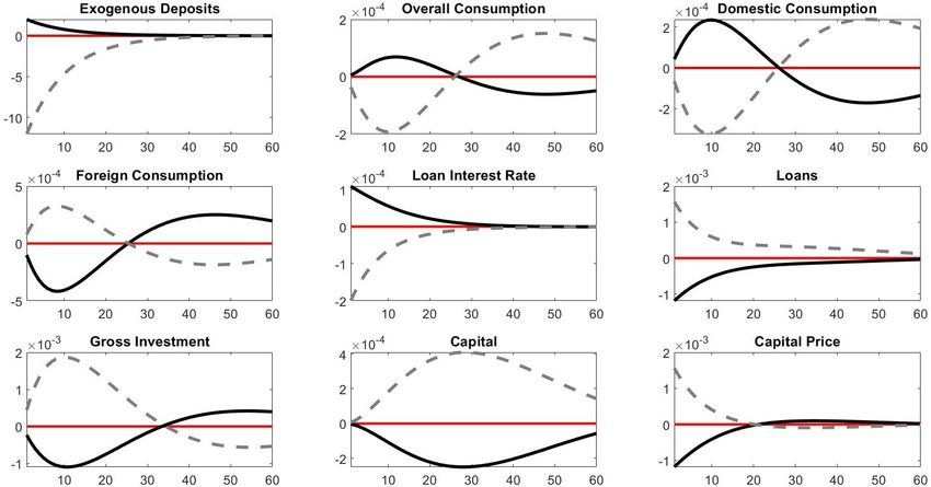
4.2.1 Preference Shock
Figure 2 depicts the impulse responses of the monetary union to a symmetric negative 1%
preference shock in countries A and B. Hence, the responses are qualitatively similar in
both countries. The preference shock implies a decrease in the households’ appreciation
of consumption, i.e., there is a decrease in their marginal utility. Thus, consumption de-
25You can also read