BIS Working Papers Funding liquidity risk: definition and measurement
←
→
Page content transcription
If your browser does not render page correctly, please read the page content below
BIS Working Papers
No 316
Funding liquidity risk:
definition and measurement
by Mathias Drehmann and Kleopatra Nikolaou

Monetary and Economic Department

July 2010

JEL classification: E58; G21

Keywords: funding liquidity; liquidity risk; bidding behavior; central
bank auctions; interbank markets
BIS Working Papers are written by members of the Monetary and Economic Department of
the Bank for International Settlements, and from time to time by other economists, and are
published by the Bank. The papers are on subjects of topical interest and are technical in
character. The views expressed in them are those of their authors and not necessarily the
views of the BIS.

Copies of publications are available from:
Bank for International Settlements
Communications
CH-4002 Basel, Switzerland

E-mail: publications@bis.org
Fax: +41 61 280 9100 and +41 61 280 8100
This publication is available on the BIS website (www.bis.org).

© Bank for International Settlements 2010. All rights reserved. Brief excerpts may be
  reproduced or translated provided the source is stated.

ISSN 1020-0959 (print)
ISBN 1682-7678 (online)
Funding liquidity risk: definition and measurement 1

                             Mathias Drehmann 2 and Kleopatra Nikolaou 3

                                         First version: December 2008
                                             This version: July 2010

                                                 Abstract

Funding liquidity risk has played a key role in all historical banking crises. Nevertheless, a
measure based on publicly available data remains so far elusive. We address this gap by
showing that aggressive bidding at central bank auctions reveals funding liquidity risk. We
can extract an insurance premium from banks’ bids which we propose as measure of funding
liquidity risk. Using a unique data set consisting of all bids in the main refinancing operation
auctions conducted at the ECB between June 2005 and October 2008 we find that funding
liquidity risk is typically stable and low, with occasional spikes, especially around key events
during the recent crisis. We also document downward spirals between funding liquidity risk
and market liquidity. As measurement without clear definitions is impossible, we initially
provide definitions of funding liquidity and funding liquidity risk.
JEL classification: E58, G21
Keywords: funding liquidity, liquidity risk, bidding behavior, central bank auctions, interbank
markets

1
    The views expressed in the paper do not represent the views of the BIS or the ECB. We would like to thank
    Claudio Borio, Markus Brunnermeier, Ben Craig, Charles Goodhart, Philipp Hartmann, Bill Nelson, Kjell
    Nyborg, Kostas Tsatsaronis, Christian Upper and Götz von Peter as well as participants at European
    Economic Association Meeting 2009, the Money, Market and Finance conference 2007, the conference on
    “Central Bank Liquidity Tools” hosted by the Federal Reserve Bank of New York, the conference on “Liquidity”
    hosted by the CESifo and Deutsche Bundesbank, the Bank of England, the Monetary Authority of Hong Kong,
    the Bank of Canada, the Norges Bank, the BIS, and the University of Pireus, Finance Division for
    helpful comments. Mathias Drehmann (corresponding author): Bank for International Settlements,
    Centralbahnplatz 2, CH-4002 Basel, Switzerland, mathias.drehmann@bis.org. Kleopatra Nikolaou: European
    Central Bank, Kaiserstrasse 29, 60311 Frankfurt am Main, Germany, kleopatra.nikolaou@ecb.int.
2
    Bank for International Settlements
3
    European Central Bank

                                                                                                              iii
Contents
Abstract.................................................................................................................................... iii
1. Introduction......................................................................................................................1
2. Definition of funding liquidity and funding liquidity risk ....................................................2
2.1. Funding liquidity and funding liquidity risk..............................................................2
2.2 Funding liquidity as a stock-flow concept...............................................................3
3. Open Market Operations in the euro area .......................................................................4
4. Funding liquidity risk and bidding behaviour at OMOs ....................................................5
4.1 Bidding with frictionless interbank markets ............................................................6
4.2 Bidding with interbank market frictions...................................................................7
4.3 Bidding with all sources of liquidity.........................................................................8
5. Measuring funding liquidity risk .......................................................................................9
5.1 Estimating the expected marginal rate and allotment volume..............................10
6. Data...............................................................................................................................11
7. Results ..........................................................................................................................12
7.1 Regression results ...............................................................................................12
7.2 The LRP measure ................................................................................................12
7.3 Funding liquidity risk and market liquidity.............................................................14
8. Discussion .....................................................................................................................15
9. Conclusion.....................................................................................................................18
Bibliography ............................................................................................................................20
Annex 1: Funding liquidity and the role of central bank money ..............................................23
Annex 2: Additional table ........................................................................................................26
Annex 3: Additional graphs.....................................................................................................27
v1. Introduction
Funding liquidity risk has played a key role in all historical banking crises. Recent events are
not different. The global credit crisis bore all the hallmarks of a funding liquidity crisis as
interbank markets collapsed and central banks around the globe had to intervene in money
markets at unprecedented levels. Nonetheless, a concrete measure of funding liquidity risk
based on readily available data remains so far elusive. This paper addresses this gap by
showing that banks’ bids during open market operations reveal funding liquidity risk.
Measurement without definition is, however, difficult if not impossible. In this paper we define
funding liquidity as the ability to settle obligations with immediacy. It follows that, a bank is
illiquid if it is unable to settle obligations in time. Consequently, we define funding liquidity risk
as the possibility that over a specific horizon the bank will become unable to settle
obligations with immediacy. In contrast to other definitions used by academics and
practitioners, our definitions have important properties, shared by definitions of other types of
risk. First, like solvency, funding liquidity is point-in-time and a binary concept as a bank is
either able to settle obligations or not. Funding liquidity risk, on the other hand, can take
infinitely many values depending on the underlying funding position of the bank. As any other
risk, it is forward looking and measured over a specific horizon.
Ideally and in line with other risks, we would want to measure funding liquidity risk by the
distribution summarising the stochastic nature of the underlying risk factors. This is
impossible as these distributions cannot be estimated because of a lack of data, even for
banks with access to more (confidential) information. Against this drawback, we propose a
new approach to measure funding liquidity risk. We extract funding liquidity risk from
observing the costs that banks are willing to pay in order to secure liquidity from the central
bank. The underlying trade-off at the central bank auction is whether to obtain liquidity from
the central bank directly or rely on other markets for liquidity. By submitting aggressive bids
at the central bank auction, the bank is very likely to obtain funds from the central bank.
Thereby it can insure against becoming illiquid. This is intuitive. But it can also be shown
theoretically that banks bid more at higher prices, the greater their funding liquidity risk
(Nyborg and Strebulaev, 2004, Välimäki, 2006). Using this insight, we show that aggregate
funding liquidity risk can be measured by the sum of the premia banks are willing to pay
above the expected marginal rate (ie the expected interest rate which will clear the auction)
times the volume they bid, normalised by the expected amount of money supplied by the
central bank. This measure can be interpreted as the weighted average insurance premium
against funding liquidity risk.
We construct our measure with the help of a unique data set of 170 main refinancing
operation (MRO) auctions, conducted between June 2005 and December 2007 in the euro
area, involving some 1055 banks. MROs have a maturity of one week, which implies that we
measure funding liquidity risk over a one week horizon. The aggregate supply of liquidity –
also called total allotment – is determined by the ECB. The auction is price-discriminating, ie
every successful bidder has to pay her bid. At the marginal rate bids may be rationed, so that
everyone takes the same pro rata amount of the remaining liquidity. The marginal rate is the
interest rate that equates aggregate demand with total allotment.
Ex ante the marginal rate is uncertain not only because the aggregate demand is unknown
but also because the ECB can adjust the supply after all bids have been received. Gauging
market expectations is a non-trivial task. The problem is further complicated by the
endogeneity between the aggregate bids and the total allotment. For this reason we rely on a
new survey dataset from Reuters, where market expectations about the marginal rate of
each auction are revealed. By nature of being survey data, the information is treated as
exogenous for all statistical purposes. To the best of our knowledge, this is the first time that
this kind of data set has been used. The expected marginal rate and other publicly available
data allow us to determine the expected total allotment.
1We find that our proposed measure has intuitive properties. Prior to the crisis, the average insurance premium was less than one basis point. Funding liquidity risk increased rapidly after August 2007 and spiked after the rescue of Northern Rock. Following the failure of Bear Sterns liquidity risk rose sharply again, even though to less elevated levels. Unsurprisingly, our measure identifies record pressures in October 2008 after Lehman failed, when the average insurance premium rose to over 40 basis points. More generally, our measure shares characteristics such as a high degree of persistence with occasional spikes, which have been documented by market participants using banks’ own models (see Matz and Neu, 2007, or Banks, 2005). Moreover, these properties are also shared by measures for market liquidity (eg see Amihud, 2002; Chordia et al., 2005; Pastor and Staumbaugh, 2003). Our measure significantly improves on other measures of funding liquidity risk. A common reference point for practitioners, policy makers and academics of the tensions prevailing during the current financial crisis have been money market spreads. We find that the EURIBOR-OIS spread is much higher than our proposed measure. This is not unsurprising as the former is affected by a host of other risk factors and therefore is not a clean measure of funding liquidity risk (eg Gyntelberg and Wooldrige, 2008). Banks’ own measures of funding liquidity risk are also not useful to measure funding liquidity risk on an aggregate basis, as they generally rely entirely on confidential information and contain a lot of judgement (eg Matz and Neu, 2007). Whilst we use confidential bidding data from the ECB, other central banks have similar data available. Furthermore, we show in the paper that a broadly similar measure of aggregate funding liquidity risk can be easily derived from public data provided by the ECB after each auction. Therefore, our method allows for a frequent and timely assessment of aggregate funding liquidity risk in an environment characterised by limited data availability. Our measure also allows us to assess the interactions of market liquidity and funding liquidity risk. Whilst this has been shown theoretically (eg Brunnermeier and Pedersen, 2009) and anecdotal evidence points to these effects in the recent crisis, the interaction between both liquidity measures has not been shown empirically due to a lack of measures for funding liquidity risk. Using our measure, we are able to show that there are strong negative interrelationships between funding liquidity risk and a measure for market liquidity. In this sense higher funding liquidity risk implies lower market liquidity. The remainder of the paper is structured as follows. In Section 2 we introduce our definition of funding and funding liquidity risk and discuss how this relates to other definitions in the literature. After providing a short overview of OMOs in the euro areas in Section 3, we show that higher funding liquidity risk will result in higher bids during OMOs in Section 4. Section 5 introduces our measure and Section 6 presents data used. In Section 7 we present the results. Further discussion is provided in Section 8. Finally, Section 9 concludes. 2. Definition of funding liquidity and funding liquidity risk 2.1. Funding liquidity and funding liquidity risk Liquidity risk arises because revenues and outlays are not synchronised (Holmström and Tirole, 1998). This would not matter if agents could issue financial contracts to third parties, pledging their future income as collateral. Given frictions, this is not always possible in reality and agents may become illiquid. We define funding liquidity as the ability to settle obligations with immediacy. Consequently, a bank is illiquid if it is unable to settle obligations. Legally, a bank is then in default. Given this definition we define funding liquidity risk as the possibility that over a specific horizon the bank will become unable to settle obligations with immediacy. It is worth to highlight important differences between funding liquidity and funding liquidity risk: Funding liquidity is essentially a binary concept, ie a bank can either settle obligations or
it cannot. Funding liquidity risk on the other hand can take infinitely many values as it is
related to the distribution of future outcomes. Implicit in this distinction is also a different time
horizon. Funding liquidity is associated with one particular point in time. Funding liquidity risk
on the other hand is always forward looking and measured over a specific horizon. In this
respect, concerns about the future ability to settle obligations, ie future funding liquidity, will
impact on current funding liquidity risk. The distinction between liquidity and liquidity risk is,
therefore, straightforward and analogous to other risks. For example, a similar distinction can
be made between credit risk and default. Whilst default either occurs or does not, credit risk
is associated with the likelihood that the borrower will default over a particular horizon. 4
Surprisingly, a distinction in the definition of funding liquidity and funding liquidity risk has not
been made by practitioners and academics so far. Borio (2000), Strahan (2008) or
Brunnermeier and Pedersen (2009) define funding liquidity as the ability to raise cash at
short notice either via asset sales or new borrowing. Whilst it is the case that banks can
settle all their obligations in a timely fashion if they can raise (sufficient) cash at short notice,
the reverse is not true as a bank may well be able to settle its obligations as long as its
current stock of cash is large enough to cover all outflows. As the ability to raise cash can
vanish (Borio, 2000) this definition is implicitly forward looking and therefore associated to
funding liquidity risk. The IMF defines funding liquidity as “the ability of a solvent institution to
make agreed-upon payments in a timely fashion” (p. xi, IMF, 2008). This definition carries the
notion that liquidity is related to the ability to settle obligations. However, it is crucial to
distinguish liquidity and solvency as welfare losses associated with illiquidity arise precisely
when solvent institutions become illiquid. The definition of the Basel Committee of Banking
Supervision is close to our definition even though it mixes the concepts of funding liquidity
and funding liquidity risk. In their view liquidity is “the ability to fund increases in assets and
meet obligations as they come due, without incurring unacceptable losses” (p.1, BCBS,
2008). The first part of this definition is essentially equivalent to ours. However, it is unclear
what ‘unacceptable losses’ really means.
Our definition raises the question how banks settle obligations. Most transactions, especially
those involving private agents, are settled in commercial bank money. However, for
transaction between banks central bank money plays a crucial role. In the Eurosystem, but
also in most other economies, large value payment and settlement systems rely on central
bank money as the ultimate settlement asset (see CPSS, 2003). 5 While banks can create
commercial bank money, the volume of central bank money is determined by central banks.
Therefore, the ability to settle obligations, and hence funding liquidity risk, is determined by
the ability to satisfy the demand for central bank money. In Annex 1 the role of central bank
money as a settlement asset is elaborated further.

2.2        Funding liquidity as a stock-flow concept 6
Based on our definition, it is easy to see that a bank is able to satisfy the demand for (central
bank) money, and hence is liquid, as long as at each point in time outflows of (central bank)

4
    A broader definition of credit risk also accounts for the stochastic nature of loss given default, changes in the
    underlying credit quality and changes in the exposure at default.
5
    Central bank money consists mainly of deposits held by commercial banks with the central bank. For a history
    of central banks’ role in interbank payment systems see Norman et al (2006). Central bank money has also
    been labelled high powered money in the monetary economics literature (eg see Friedman and Schwarz,
    1963).
6
    This section draws on earlier unpublished work by Drehmann, Elliot and Kapadia, which is now incorporated in
    Kapadia et al (2010).

                                                                                                                   3
money are smaller or equal to inflows plus the stock of (central bank) money held by the
bank:
Outflowst ≤ Inflowst + Stock of Moneyt (1)
Annex 1 provides a more detailed breakdown of in- and outflows. For now, we focus on the
net volume of money needed to avoid illiquidity. We construct the net-liquidity demand (NLD)
from the stock flow constraint above. Namely, we take the difference between all outflows
(Outflows) and contractual (ie known) inflows (Inflowsdue) net of the stock of central bank
money (M):
NLDt Outflowst Inflowstdue M t
(2)
ptD LDnew,t ptIB LIB
new,t pt Asold ,t pt CBnew,t
A CB
In case of a deficit (ie outflows are larger than inflows and the stock of money), the inequality
highlights that NLDt has to be financed either by new borrowing from depositors ( LDnew ), from
the interbank market ( LIB
new ), selling assets (Asold) or accessing the central bank (CBnew). All
these sources have different prices p. If there is a positive net liquidity demand which cannot
be funded with new inflows, the bank will become illiquid and default. Conversely, if the bank
has an excess supply of liquidity, no borrowing is necessary and the bank can sell the
excess liquidity on the market. Note that this means that ex-post inflows always equal
outflows, as long as the bank does not fail. But ex-ante, equation (2) highlights that funding
liquidity risk is driven by two stochastic components: future developments of NLD (ie
volumes) and future prices of liquidity in different markets.
The question for this paper is how to measure funding liquidity risk. Ideally, and in line with
other risks, we would want to measure funding liquidity risk by the distribution jointly
summarising the stochastic nature of in- and outflows as well as prices. But, even banks with
access to far more data are unable to construct such a distribution. For example, it is
impossible to estimate prices of, and access to, liquidity in different markets in stressed
conditions, as crises occur too rarely to use standard statistical tools.
We propose a different approach to measure funding liquidity risk, which incorporates
information on both volumes and price of liquidity. We observe banks’ bids (rates and
volumes) during central bank operations (or ptCB CBnew,t in the language of equation (2)). In
Section 4 we explain that banks with higher funding liquidity risk will bid more aggressively,
and the more so, the higher their funding liquidity risk. A short overview over the institutional
background of open market operations (OMOs) in the euro area may be useful in that
respect.
3. Open Market Operations in the euro area
We use data from 1 June 2005 until 10 October 2008. During this time OMOs are mainly
conducted as short-term main refinancing operations (MROs) or longer-term refinancing
operations (LTROs). MROs are carried out weekly and have a maturity of one week.
Traditionally MROs have provided the main bulk of liquidity to the euro area. 7 Additionally,
7
This has changed with the onset of the crisis in August 2007, when the heightened uncertainties lead to an
increase in the liquidity demand for longer horizons.the ECB can undertake fine-tuning operations in case of a need for an additional and
extraordinary injection or absorption of central bank money.
MROs form the basis of our measure. Note that this means that we measure funding liquidity
risk over a one week horizon. In our sample, MROs are conducted as variable rate tenders. 8
The auction set-up is as follows: Eligible banks can submit bids (volume and price) at up to
ten different bid rates at the precision of one basis point (0.01%). Prices and volumes are
unconstrained, except for the minimum bid rate, which equals the policy rate set by the
Governing Council. The aggregate supply of liquidity – also called total allotment – is
determined by the ECB. The auction is price-discriminating, ie every successful bidder has to
pay her bid. The marginal rate is the interest rate when aggregate demand equals supply. At
the marginal rate, depending on the aggregate bid schedule, bids may be rationed, so that
everyone takes the same pro rata amount of the remaining liquidity. Banks are only required
to submit sufficient collateral for the allotted liquidity.
Under normal conditions, the total allotment in the weekly MROs is determined by the
benchmark allotment. This is the volume that satisfies exactly these needs for central bank
money in aggregate and is calculated as the sum of the autonomous factor forecasts (such
as banknotes, government deposits and net foreign assets) and banks' reserve
requirements. 9 This forecast, technically called benchmark at announcement, is published
prior to the auction. The ECB can deviate from the forecast and provide more or less liquidity
after it received all the bids, even though the distribution of deviations is skewed towards the
positive side. As central bank operations are primarily monetary policy operations with a
purpose to steer market rates close to the policy rate, the ECB made use of this option to a
larger extent after the beginning of the crisis. During this period the ECB “front-loaded”
liquidity requirements. Front loading is an allotment practice, where the central bank provides
liquidity above the benchmark in the beginning of the maintenance period, and close to or
just below the benchmark towards the end of the maintenance period, possibly in
combination with liquidity absorbing operations. In doing so, the central bank makes sure that
banks fulfil their reserve requirements early in the maintenance period. In times of crisis this
helps to stabilise the overnight rate. Clearly, market participants try to anticipate the ECB
behaviour when submitting bids. We take this endogeneity into account when constructing
our measure (see Section 5).
4. Funding liquidity risk and bidding behaviour at OMOs
In this section we show that funding liquidity risk is revealed by the price banks are willing to
pay during open market operations. In particular we show that aggregate liquidity risk can be
measured by the sum of the premia banks are willing to pay above the expected marginal
8
In October 2008 the ECB changed the tender procedure to full allotment at the fixed rate prevailing at the
MRO, following the intensification of the crisis in the immediate aftermath of the Lehman collapse. Under the
new framework, only the volumes of liquidity demand are revealed but not the price. As a result, our measure
as presented here does not apply on the new auction design after October 2008. However, we conjecture that
volumes bid still reveal funding pressures as the rates in the interbank markets for “good” banks are below the
policy rate.
9
In the Euro area individual banks have to fulfil reserve requirements. Banks are allowed to hold positive or
negative (relative) reserve balances with the CB within a specified period; ie relative to their requirements
banks can hold more or less. Negative current accounts, so-called intraday credit, have to be collateralised
and will be referred to the marginal lending facility at the end of the day. Reserve requirements have to be
fulfilled on average across the maintenance period (usually between 28 and 35 days). At the start of the
maintenance period the reserve requirements are determined by the Eurosystem for each bank and remain
fixed during the period
5rate times the volume they bid, normalised by the expected total allotment. This measure can
be interpreted as the weighted average insurance premium against funding liquidity risk.
The theoretical literature assessing the bidding behaviour of banks during open market
operations started with Poole (1968). It generally considers a stylised time line. In the
simplest case, it consists of three periods (see Figure 1). In period 1, banks can acquire
liquidity in the primary market by participating in the auction conducted by the central bank.
Afterwards liquidity shocks materialise. In period 2, banks trade in the interbank market. After
interbank markets close in period 3, all obligations are settled and banks have to fulfil their
reserve requirements set by the central bank. 10 At this point the market in aggregate may be
short (or long) of liquidity and hence some banks may have to access the marginal lending
(deposit) facility. Prices for the marginal facilities are considered key policy rates and are
determined by the central bank, therefore they are already known in period 1. At the same
time, these prices constitute an upper and lower bound for the interest rate in the interbank
market in period 2, given that a bank with sufficient collateral can always recourse to the
standing facilities at period 3 to settle any liquidity imbalances. For our sample period, banks
paid 100bp on top of (below) the policy rate to access the marginal lending (deposit) facility.
Figure 1
Stylised time line
Period 1 Primary market: Auction conducted by central bank
Liquidity shocks
Period 2 Secondary market: trading in the interbank market
Period 3 Final settlement: banks can access marginal facilities at the central bank
To assess the bidding behaviour of banks and how this relates to liquidity risk, it is important
to distinguish interbank markets with and without frictions. Note, that throughout the
discussion we only consider price discriminating auctions, which is the auction design used
by the ECB. Moreover, we follow the literature and assume throughout the theoretical
discussion that the central bank accurately provides the necessary and known (expected)
amount of central bank money, independent of the bids it receives.
4.1 Bidding with frictionless interbank markets
If interbank markets are frictionless and banks are risk neutral, Välimäki (2002) and Ayuso
and Repullo (2003) show that it is optimal for banks to only bid at the minimum bid rate. No
bank is, therefore, willing to pay a premium above the minimum bid rate.
This result is intuitive. First consider the case where banks are only subject to idiosyncratic
liquidity shocks so that there is no aggregate liquidity surplus or deficit in period 2 or 3. As
10
Most countries have positive reserve requirements for banks. However, theoretically it is only necessary that
there is a threshold, eg zero, and banks would be penalised if their balances with the central bank would drop
below this level.long as banks are solvent, banks can always obtain the required funding in the secondary
market as the (frictionless) interbank market allocates liquidity from those with a surplus to
those with a deficit. Given the central bank provides the right amount of liquidity, the interest
rate in the interbank market equals the minimum bid rate. With no uncertainty in period 2,
bidding at the minimum bid rate in period 1 is the only rational strategy. Hence, our
suggested measure would indicate zero liquidity risk, which is exactly what it should do.
Theory has shown that funding liquidity risk is zero when interbank markets are frictionless
and no aggregate shocks occur (eg Allen and Gale, 2000).
Even with frictionless interbank markets, however, trading cannot eliminate the risk that the
market on aggregate may be long or short of central bank money in period 3. As prices for
accessing the marginal facilities are fixed, the interest rate in period 2 purely reflects the
expectations of the amount and likelihood of accessing either facility in period 3. But at time 1
banks expect that the interest rate in the interbank market equals the policy rate, as the
central bank is assumed to provide the right expected amount of aggregate liquidity. Given
risk neutrality, all banks therefore bid at the minimum bid rate as they are indifferent between
obtaining liquidity in the primary auction or from the interbank markets. Hence, our proposed
measure would indicate no risk. However, the assumption of risk neutral banks and
frictionless interbank markets is unrealistic, particularly during times of stress. If we relax
these assumptions, higher bids reveal higher liquidity risk.
4.2 Bidding with interbank market frictions
It has been theoretically shown that asymmetric information (eg Flannery, 1996), co-
ordination failures (eg Rochet and Vives, 2002), uncertainly about future liquidity needs (eg
Holmstrom and Tirole, 2001) or incomplete markets (eg Allen and Gale, 2000) are all frictions
which lead to funding liquidity risk. Such frictions imply that a bank which has to raise liquidity
in the interbank market may have to pay more than the market rate to obtain it. In the
extreme, prices may even be “infinite” if a bank is rationed (see Stiglitz and Weiss, 1981) or
markets break down completely (Heider et al, 2009, or Diamond and Rajan, 2009). 11
Banks with high liquidity risk anticipate this before they submit their bids. The underlying
trade-off is whether to obtain liquidity from the central bank (period 1 in Figure 1) or rely on
other markets for liquidity (period 2), which may be very costly. By submitting aggressive bids
at the central bank auction, the bank is very likely to obtain funds from the central bank.
Thereby it can insure itself against becoming illiquid. It is intuitive that a bank with higher risk
is willing to pay a higher premium. Nyborg and Strebulaev (2004) show formally that, “short”
banks (ie banks which do need to raise cash from the central bank or the interbank market to
settle all obligations) will bid more aggressively than “long” banks (ie banks which have
excess funds), even if all banks are risk neutral. 12 In particular, Nyborg and Strebulaev
analyse the case where long banks have some market power during trading in the secondary
11
Nikolaou (2009) provides an overview over the literature describing the role of interbank markets and funding
liquidity risk.
12
Formally, the results from Nyborg and Strebulaev will only carry over to a setting with a different interbank
market frictions, if the friction implies that long players can charge a higher interest rate if short banks are
sufficiently illiquid. If the interbank market is closed and only banks can trade in the interbank market this is the
case. Nyborg and Strebulaev also assume that agents have full information on short and long positions prior
to the OMO. However, imperfections in the interbank market are often associated with imperfect information.
Nyborg and Strebulaev conjecture that with private information about positions, long players will aim to exploit
their informational advantage. But in equilibrium short banks would still bid on average at higher rates to
prevent the squeeze.
7market, so that they can “squeeze” short banks and demand higher interest rates. 13 Short
banks can avoid being squeezed if they obtain sufficient funds from the central bank during
the OMO. And to ensure that they get the required funds, they have to bid above the
expected marginal rate. Nyborg and Strebulaev show that in equilibrium the threat of a
squeeze induces short banks to submit on average bids above the minimum bid rate with a
higher expected mean rate than the bids submitted by banks which are long. The authors
also show, that the larger the short position, the larger are the volumes bid at higher prices. 14
Or putting it simply, banks bid more at higher prices, the greater their funding liquidity risk.
Aggressive bidding may also occur because banks may not be risk neutral. Once a bank
becomes illiquid, it will default. It is therefore likely that is some circumstances the bank will
act as if it is risk averse. Obviously, risk aversion implies that banks with high liquidity risk will
pay a higher premium to insure against this risk. During normal times the effects of risk
aversion should not be material as interbank markets are nearly frictionless and banks can
obtain any required amount of funding in the secondary market. The only risk banks face, are
small price changes for unsecured lending due to small aggregate shocks. 15 However, in
stressed conditions the risk of becoming illiquid or having to pay high costs to obtain funds in
the secondary market increases, so the effects of risk aversion on bid behaviour are more
important.
Välimäki (2006) explores a model with risk averse banks, where deviations from a target
level of central bank balances prior to trading in the interbank market are costly. Such a
target level could be the result of frictions. For example, banks know that the desire to obtain
very large amounts of money would be penalised by rates above the market rate or it may
even be impossible to raise the necessary amount of funds because of rationing. In line with
Nyborg and Strebulaev, Välimäki shows that banks with a higher target level, or equivalently
with a higher NLD, bid more aggressively during the central bank auction. Again the more
banks bid at rates above the expected marginal rate, the greater their funding liquidity risk.
4.3 Bidding with all sources of liquidity
No model in the literature on bidding behaviour in OMOs takes account of all sources of
funding liquidity shown in equation 2. In reality, banks can trade in the interbank market but
also obtain liquidity from depositors or from selling assets. However, within the one week
horizon we consider here, banks cannot expect to rely on new customer deposits to weather
unexpected liquidity shocks. In the short run, banks have a limited ability to attract a
significant amount of new customer deposits (for example by raising rates) because of
sluggish depositors’ behaviour (see Gondat-Larralde and Nier, 2004).
Asset sales are therefore the only other alternative source of liquidity in the short run.
Without frictions in any market, the costs of obtaining liquidity from the interbank market or
from selling assets are equal as all price differentials are arbitraged away. In such an
environment, the results from Section 4.1 apply and banks only bid at the policy rate. But as
in the case of interbank market, frictions in asset markets are central in theories of liquidity
13
Acharya et al (2008) document several banking crises where this effect seems to have played an important
role.
14
Fecht et al. (2009) find empirical support for this by analysing OMOs for German banks. They document that
banks, which are below their reserve requirements, bid more aggressively especially in times when the
imbalance across banks is large.
15
As long as all banks lend freely in the interbank market, aggregate liquidity shocks in the market for central
bank money are technically only driven by changes in autonomous factors. Autonomous factors constitute
(nearly completely) of banknotes, government deposits and net foreign assets. These factors can and do
change between OMOs even though these fluctuations are generally not large.risk (for an overview see eg Biais et al, 2005). In case of frictions in both asset and interbank
markets, downward spirals between market and funding liquidity can emerge (Brunnermeier
and Pedersen, 2009). A downward liquidity spiral can, for example, start with a bank (or
brokers in the Brunnermeier and Pedersen model), which is short of funding liquidity and
cannot obtain it from the interbank market. Therefore, it has to sell assets. If asset markets
are characterised by frictions, (large) asset sales induce a fall in asset prices. These in turn
imply that the bank has to post higher margins, which increases liquidity outflows. To remain
liquid banks have to sell even more assets, which depresses market prices even further
(because of a lack of market liquidity), leading to further margin calls and so forth. Banks with
high liquidity risk will expect these effects. Therefore, they will bid more aggressively in the
primary auction to obtain the required funds. Using our proposed measure of funding liquidity
risk, we show that these downward spirals can actually be documented during the crisis.
Before we turn to the empirical analysis we should point out that our measure of funding
liquidity risk may also be influenced by other factors. First, there could be collateral effects as
the ECB accepts a larger pool of collateral than can be used in the securitised interbank
markets. We do not expect this to bias our results in a significant fashion, as interbank
markets work to a large extend on an uncollateralised basis. 16 Second, it has been shown
that at year-ends, banks bid more aggressively to engage in window-dressing and establish
favourable end of year balances (see Bindseil et al 2003). Clearly, such seasonality effects
are unrelated to liquidity risk as they are not driven by a reaction to funding pressures. This,
however, affects primarily year-end auctions, which we therefore drop.
Third, bidding behaviour may also be influenced by the well-known “winner’s curse” problem
which results in underbidding (eg see Milgrom and Weber, 1982). 17 For this problem,
however, to be material it is necessary that market participants have asymmetric information
about the value of the good in the secondary market. Bindseil et al. (2009) find no evidence
that this is the case for OMOs in the euro area. Hence, the winner’s curse problem should
not impact on our measures.
5. Measuring funding liquidity risk
In Section 4 we have shown that large bid volumes at prices above the expected marginal
rate reveal funding liquidity risk as a bidder can be relatively certain that she will get the
liquidity requested without being rationed. 18 Our measure is, therefore, simply based on the
volume banks bid at rates above the expected marginal rate.
We define the adjusted bid (AB) as
16
The broad collateral framework of the ECB may render the ECB auctions relatively more attractive than the
secured money market. Ewerhart at al (20010) show theoretically that this may lead banks to bid more
aggressively. During normal times this effect should not be large as liquidity is readily available in all money
market segments. In crisis the may be different. However, during the recent crisis , the ECB has broadened its
collateral eligibility rules to accommodate the large liquidity demand of the banking system, given the
breakdown of several money market segments. Therefore, it is unclear what the net-effect is on our measure
during the crisis.
17
In a multi-unit set-up the winner’s curse problem is referred to as champion’s plague (Ausubel, 2004).
18
In theory, the expected marginal rate equals the minimum bid rate. However, the marginal rate has been on
average 6 bps above the policy rate even in normal times. In section 5.1 we will explain in detail how we
measure the expected marginal rate as well as the expected total allotment empirically.
9ABb ,i ,t (bid _ rateb ,i ,t E (marginal _ rate) t ) * volumeb ,i ,t
(3)
if bid _ rateb ,i ,t E (marginal _ rate) t
where, bid _ rateb ,i ,t and volumeb ,i ,t are the rate and volume of bank i (from 1 to N ), which
submits b bids (from 1 to B) at time (auction) t. E (marginal _ rate)t is the expected marginal
rate. ABb,i,t are the total costs a bank is willing to pay to ensure that it obtains the volumeb,i,t of
cash from the central bank. In this sense, it is an insurance cost against funding liquidity risk.
Given AB it is easy to construct an aggregate liquidity risk insurance premia (LRP) by
summing across all adjusted bids of all banks.
N B
AB b ,i ,t
(4)
LRPt i 1 b 1
* 100
E( allotment )t
We normalise the sum of the adjusted bid rates by the volume banks expect the central bank
to provide. The normalization is necessary to ensure consistency across auctions which
differ in size. This will also ensure that our measure is unaffected by “frontloading” practices
after August 2007 as discussed in Section 3. Furthermore, the normalisation implies that
LRP is the value weighted average spread banks are willing to pay to ensure that they obtain
liquidity from the central bank. Or putting it simply LRP is the average insurance premium
banks are willing to pay to insure against funding liquidity risk. The multiplication by 100
implies that it is measured in basis points. An alternative interpretation is shown in Graph
A3.1 using one auction as an example. As can be seen LRP is simply the normalised area
under the aggregate demand curve.
5.1 Estimating the expected marginal rate and allotment volume
As we discussed previously, the central bank can adjust the supply of liquidity after all bids
have been received. The market will anticipate this when forming their expectations about
the marginal rate and the total allotment volume, which we require as inputs for our measure.
Gauging market expectations is a non-trivial task. The problem is further complicated by the
endogeneity between the aggregate bids and the total allotment. For this reason we rely on a
new survey dataset from Reuters, where market expectations about the marginal rate of
each auction are revealed (these data are described in detail in Section 6). Using this data
set we can treat the expected marginal rate as an exogenous variable to determine the
expected total allotment (TA) by a simple OLS regression:
TAt 0 1 * E( spread )t 2 * benchmark 4 * end t (5)
All regressors in equation (5) are known when bids are submitted. E(spread) is the expected
spread between the expected marginal rate and the policy rate, which is known before bids
are submitted. 19 benchmark is the benchmark at announcement. At the end of the
maintenance period it is likely that the behaviour of the allotment volume is different as the
excess liquidity has to be balanced out. To account for this we insert a dummy variable end
which equals 1 on the last auction of each maintenance period.
19
The policy rate is set on the monthly meetings of the Governing Council of the ECB. It is announced on the
first Thursday of every month and is valid for the maintenance period that spans the period during two
consecutive announcements. It is effective from the MRO immediately following the announcement and for all
consequent MROs within the same maintenance period.We use a 30-day rolling window estimation procedure. Rolling windows estimation is ideal in
case of structural breaks in the data, which are likely to exist given the outbreak of the
crisis. 20 We choose a 30 day window as this provides us with the necessary amount of data
in order to achieve efficient asymptotic estimates, while at the same time it minimises the
effects of changes which occurred during the crisis, for which we only have 59 observations.
6. Data
Our analysis benefits from a unique data set of 175 MROs conducted by the ECB from June
2005 to 7 October 2008. To avoid the contamination of our measure by window-dressing, we
drop the last operation in each year. We also do not consider the operation conducted on 18
Dec 2007 as this had a maturity of 2 weeks. In total we have therefore 171 MROs in our
sample.
Overall, 1055 banks took part at least once in any of these auctions. We have information on
an anonymous but unique code for each bidder, the submitted bid schedule (bid rate and bid
volume) of each bank and the allotted volume. These data are not publicly available.
However, data on the policy rate (minimum bid rate), the marginal rate, the maintenance
periods, the benchmark and the settlement dates of the auctions are publicly available and
taken from the ECB's internet site. 21
We combine this information with data from a Reuters poll surveying expectations of the
marginal rate. To our knowledge, this is the first time these data are used. The poll is
conducted on a weekly basis. Reuters asks a number of banks (usually the same panel of 25
to 30) every week about their expectations about the marginal rate. These banks represent
the largest banks in the euro area as well as some mid-size dealers. The number of
banks may vary slightly per week depending on availability. We use the mean of this survey
as the expected marginal rate. Graph 1 shows that before the crisis, the market anticipates
the marginal rate well. Afterwards a gap emerges. Interestingly, the market seems to
consistently underestimate the marginal rate in the early stages of the crisis.
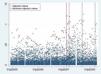
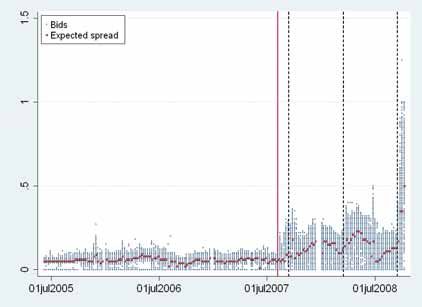
Graph A3.2 in the Annex provides an overview over the components of the individual bids.
The left-hand panel shows the individual bid rates as spreads above the minimum bid rate.
Each data point corresponds to a single dot in the graph. It is apparent that the crisis period
is associated with a larger variability in bid rates and more aggressive bidding as suggested
by the amount and extent of bids above the expected marginal rate. The right-hand panel of
Graph A3.2 shows the volumes bid for bid rates above the expected marginal rate. In line
with equation 4, we normalise each submitted bid volume by the expected total allotment. In
contrast to the rates, volumes bid do not change dramatically before and during the crisis,
even though some increase is apparent.
Graph A3.3 presents the evolution of the total allotment and the benchmark at
announcement. Prior to August 2007 the benchmark is a very good predictor for the actual
allotment. On average, the difference during this period is only 0.4%. This changed with the
beginning of the crisis, when the ECB started the frontloading practices described in
Section 3.
20
Windows of length 24, 40, 50, 52 and 60 observations were also tried. Results are broadly similar and
available on request.
21
http://www.ecb.eu/mopo/implement/omo/html/index.en.html
117. Results
7.1 Regression results
Before moving on to present LRP we briefly present the results of the regression determining
the expected allotment as described in equation (5). Graph 1 below shows the actual versus
fitted values and the R2.
As a general result the fit is rather good. Before the crisis the total allotment can be nearly
perfectly forecasted as the benchmark at announcement is very close to the actual allotment.
During the crisis the fit continues to be quite good (around 80%), with the notable exceptions
of the outbreak of the turmoil in August 2007 and the incident of the Lehman collapse at the
end of our sample. These two exceptions are technically grounded, given the structural
breaks in the data (validated by appropriate Chow tests) and are also economically
reasonable, given that both incidents occurred suddenly and therefore expectations about
volumes would consider only the pre-crisis information set.
Graph 1
Total allotment and the marginal rate: Expected versus actual
Total allotment1 Spread between the actual and expected marginal
rate2
350000
.5
1
Actual
Expected
300000
.4
.8
250000
.3
.6
.2
200000
.4
.1
150000
Actual
Fitted
R2 (right axis)
.2
0
01jul2005 01jul2006 01jul2007 01jul2008 01jul2005 01jul2006 01jul2007 01jul2008
1
Regressions are based on 30 observations rolling window. For each rolling regression, we show the last
predicted value, except for the beginning of the sample where we use the first regression to derive the
2
predicted values. Expected rates are taken from the Reuters poll. The red horizontal line indicates the
beginning of the crisis (7August 2007).The horizontal black lines indicate dates of important events, the failure
of Northern Rock (13 September 2007), the failure of Bearn Sterns (16 March 2008) and the failure of Lehman
Brothers (15 September 2008).
7.2 The LRP measure
Our aggregate measure of funding liquidity risk is presented in Graph 2. Unsurprising, LRP
reveals that liquidity risk is much greater and has much more pronounced spikes towards the
end of our sample. The change in level coincides perfectly with the beginning of the crisis.
Prior to the crisis, banks on average paid below 1 basis point to insure against funding
liquidity risk (see Table 1). The average insurance premium increased rapidly after August
2007, and reached a first peak of more than 16 basis points after Northern Rock had to be
rescued by the UK government. A relative tranquil period followed, but liquidity risk rose
again at the end of the year. The failure of Bear Sterns, was also followed by a pronounced
spike, even though this was less significant than the spike following the failure of Northern
Rock. Tensions subsequently subsided but rose towards the end of June 2008. To someextent this may reveal window dressing effects and uncertainties about half year results. The
largest spike in funding liquidity risk occured at the beginning of October 2008, when money
markets broke down completely following the failure of Lehman Brothers. At this point, the
average insurance premium was more than 44 basis points (see Table 1).
The graph clearly shows that funding liquidity risk is time varying and persistent, but subject
to occasional spikes. These characteristics have been documented by market participants
using banks’ own models (see Matz and Neu, 2007, or Banks, 2005), but are also common
for measures of market liquidity (Amihud, 2002; Chordia et al., 2005; Pastor and
Staumbaugh, 2003).
Graph 2
LRP
40
30
20
10
0
01jul2005 01jul2006 01jul2007 01jul2008
Note: The red horizontal line indicates the beginning of the crisis (7 August 2007).The horizontal black lines
indicate the failure of Northern Rock (13 September 2007), the failure of Bearn Sterns (16 March 2008) and the
failure of Lehman Brothers (15 September 2008). In basis points.
Table 1
Statistics of the liquidity risk
LRP
Normal Crisis Ratio
Mean 0.9 7.6 8.7
Std. 0.4 7.1 19.1
Min 0.1 2.7 20.0
Max 2.2 44.1 19.9
# Observations 112 59
Note: Normal indicates the period from June 2005 until 7 August 2007. Crisis is the remaining period until 7
October 2008. Ratio equals Crisis/Normal. LRP is measured in basis points.
137.3 Funding liquidity risk and market liquidity
As discussed in Section 4.3 market and funding liquidity are strongly interrelated and
downward spirals of market and funding liquidity risk can emerge in crises. Whilst the
theoretical expositions are clear and anecdotal evidence points to these effects in the recent
crisis, the interaction between both liquidity measures has not been shown empirically due to
a lack of measures for funding liquidity risk.
Using our measure we are able to assess this question in a more robust fashion. We use a
broad measure of market liquidity for the euro area (see ECB, 2007) which is shown in
Graph A3.4 (left-hand panel) in the Annex. This index of market liquidity is a weighted
average of different market liquidity measures such as bid-ask spreads in FX, equity, bond
and money markets. 22
Graph 3 shows a scatter plot of LRP and the market liquidity index. A clear negative
relationship can be seen, ie when market liquidity is drying up (ie is low), funding liquidity risk
is high (which would be equivalent to saying that high funding liquidity risk is associated with
high market liquidity risk). The orange and green lines show the predicted values based on a
simple regression of the index on LRP during normal times and the crisis.
Graph 3
Interactions between funding liquidity risk and market liquidity
Normal
Crisis
40
Normal: Fitted values
Crisis: Fitted values
30
LRP
2010
0
-3 -2 -1 0 1
Market liquidity index
Note: Normal indicates the period from June 2005 until 7 August 2007. Crisis is the remaining period until 7
October 2007. Fitted values are based on the regression using the specified sub-samples.
22
As discussed in ECB (2007) (Box 9), “the financial market liquidity indicator combines eight individual liquidity
measures. Three of them cover bid-ask spreads: (1) on the EUR/USD, EUR/JPY and EUR/GBP exchange
rates; (2) on the 50 individual stocks which form the Dow Jones EURO STOXX 50 index and; (3) on EONIA
one month and 3 month swap rates. Three others are return-to-turnover ratios calculated for: (4) the 50
individual stocks which make up the Dow Jones EURO STOXX 50 index; (5) euro bond markets and; (6) the
equity options market. The last two components which measure the liquidity premium are gauged by: (7)
spreads on euro area high-yield corporate bonds which are adjusted to take account of the credit risk implied
in these spreads by expected default frequencies (EDFs) and; (8) euro area spreads between interbank
deposit and repo interest rates. The composite indicator is a simple average of all the liquidity measures
normalised on the period 1999-2006”.The regression results are shown in Table 2. The scatter plot already suggests that the
negative relationship only emerges during the crisis. The econometric analysis supports this
as there is no significant relationship between our measure of funding liquidity risk and
market liquidity prior to the crisis. 23 However, once the crisis unfolds a significant negative
relationship emerges. This is exactly what the theory predicts as these interactions should
only emerge once banks become funding constraint. The relationship during the crisis is also
economically significant. The estimates imply that for example a fall of the market liquidity
index by 3 standard deviations is associated with a 14 basis points increase in the average
liquidity insurance premium. This is approximately the difference between levels of LRP after
the failures of Northern Rock or Bear Sterns and pre-crisis levels. Note that we do not want
to imply any causal relationships with this thought experiment as market and funding liquidity
risk are determined simultaneously in equilibrium.
The market liquidity index used above combines different money market liquidity measures,
which we can separate into two composite indices, namely a FX, equity and bond markets
index and a money market index. Given the nature of the crisis, it is plausible that our results
are driven by developments in money markets. However, our results hold, even when we
focus solely on the composite index of FX, equity and bonds markets (see Table A2.1 in the
Annex).
Table 2
Regression results of LRP on the market liquidity index
Coefficient R-squared Observations
Full sample
Market liquidity -5.7*** 0.48 171
Constant 2.5***
Normal
Market liquidity -0.4 0.003 112
Constant 1.0***
Crisis
Market liquidity -5.3*** 0.17 59
Constant 2.9*
The independent variable is LRP for all regressions. Normal indicates the period from June 2005 until 7 August
2007. Crisis is the remaining period until 7 October 2008. *** significant at the 1% level, ** significant at
the 5% level, * significant at the 10% level.
8. Discussion
Ideally, we would provide a comparison with banks’ own measures of funding liquidity risk
and how this relates to their bidding behaviour. However, this information is unavailable. A
typical measure commonly used by central banks, academics and practitioners to assess
23
To see whether the results are driven by outliers, we dropped the 5% highest LRP values in the sample as a
robustness check. We continue to find the same qualitative results.
15You can also read