Multiscale Systemic Risk and Its Spillover Effects in the Cryptocurrency Market

Hindawi
Complexity
Volume 2021, Article ID 5581843, 22 pages
https://doi.org/10.1155/2021/5581843

Research Article
Multiscale Systemic Risk and Its Spillover Effects in the
Cryptocurrency Market

 1 2
 Xu Zhang and Zhijing Ding
 1
 School of Management Science and Engineering, Nanjing University of Information Science and Technology,
 Nanjing 210044, China
 2
 Chang Wang School of Honors, Nanjing University of Information Science and Technology, Nanjing 210044, China

 Correspondence should be addressed to Zhijing Ding; 201883200001@nuist.edu.cn

 Received 16 February 2021; Revised 8 May 2021; Accepted 20 May 2021; Published 1 June 2021

 Academic Editor: Ning Cai

 Copyright © 2021 Xu Zhang and Zhijing Ding. This is an open access article distributed under the Creative Commons Attribution
 License, which permits unrestricted use, distribution, and reproduction in any medium, provided the original work is
 properly cited.
 Since the advent of Bitcoin, the cryptocurrency market has become an important financial market. However, due to the existence
 of the cryptocurrency bubble, investors face more difficulties in risk portfolios. We adopt wavelet packet decomposition, nonlinear
 Granger causality test, risk spillover network, and STVAR model; retain the mature research of multiscale systemic risk based on
 time and frequency; and thus extend systemic risk to different regimes. We found that when frequency is combined with regimes,
 the risk spillover center will undergo subversive changes in the long run. We also proposed that BTC will be more robust at
 extreme values (like longest and shortest periods), while cryptocurrencies with smaller market capitalization will be stronger in the
 medium term. At the same time, the recession period will also spur on it.

1. Introduction Banking Crisis of Cyprus in 2012-2013 [5]. Importantly, the
 literature believes that Bitcoin has a very weak relationship
In 2009, Nakamoto [1] proposed the concept of crypto- with traditional assets, which makes it a valuable diversifier
currency and a proof system for encrypted payment. Thanks [7, 8] and in some cases a hedge or a safe haven against
to its blockchain technology, Bitcoin does not involve equities [6]. Excluding the asymmetric response in variance,
intermediaries such as clearinghouses and is thus inde- Klein et al. [9] argue that cryptocurrencies are the same as
pendent of sovereign risk [2]. At the same time, in 2017, the gold in volatility, correlation, and portfolio performance,
CME Group and the CBOE launched futures contracts with which makes it a probable alternative. With the increasingly
Bitcoin as an underlying asset, legitimizing it further. This close connection with other markets, its volatility has be-
has allowed Bitcoin to join commodities, including gold, in come a hot topic for scholars.
futures trading, and eventually move from the margins to the Investors’ expectations for Bitcoin’s risk aversion
center of the financial world [3]. Accordingly, the crypto- characteristics seem to be broken in the risk of contagion.
currency market has gradually gained much attention from Kyriazis et al. summarized the volatility and persistence of
speculators, investors, technology enthusiasts, and even the cryptocurrency bubbles using a literature review, revealing a
public. Due to its nonpolitical nature and commodity at- strong confounding effect on its guidance on financial
tributes [4], Bitcoin, the cryptocurrency of largest market markets [10]. Fry and Cheah [11] used mathematical fi-
value, is often compared to gold, which serves as a safe haven nancial models to deduce that financial events strike based
for investors to carry out risk portfolios [5]. Bitcoin is often on the size and degree of BTC bubbles, even a negative
seen as a panacea, replacing financial institutions, and bubble. The alternating surge of Bitcoin and Dogecoin
providing shelter for sovereign risk and weakness in the proves this bubble effect. In contrast to stock indices, Cheah
global financial system [6], especially during the surge in the et al. [12] find that BTC builds speculative bubbles, affecting

2 Complexity

the extent to which it functions as a weak or strong safe from the perspective of the theoretical framework of sys-
haven. When the cryptocurrency market enters an uptrend, temic risk, we provide feasible research ideas and improve
the rise in exchange rates actively increases the comovement the nonlinear research based on systemic risk. In the
of cryptocurrencies, thus limiting investors from taking nonlinear stage, the STVAR model with embedded state
advantage of diversification. Enoksen et al. [13] measured variables was introduced, the changes within the regime
the bubble cycles of eight cryptocurrencies, verifying the were examined, and the current shortage of the Markov
rationality of cryptocurrencies surging at the beginning of matrix used in the current stage was corrected, and the
2018. They also determined that higher volatility, volume, innovation of the research model from time to frequency to
and transactions are positively correlated with the bubbles regime was achieved. Second, from the perspective of aca-
between cryptocurrencies, which lay a possible explanation demic research, we use the cryptocurrency market index
for dynamic in the cryptocurrency market. In 2020, COVID- (CRIX) as a state variable to consider the influence under
19 is prevalent, scholars pointed out that the epidemic different regimes brought by the cryptocurrency market and
caused the fluctuation of Bitcoin prices [14–16]. With the also enlighten the possible directions of future research:
gradual dissipation of this major health incident, the rela- introducing other macro variables closely related to the
tionship between macroeconomic events and the crypto- cryptocurrency market as state variables. At the same time,
currency market has attracted attention. Combining wavelet optimizing wavelet decomposition into wavelet packet de-
decomposition and Granger causality test, Li et al. [17] found composition is a generalized measure. Third, from the
time asymmetry in the causal relationship between the perspective of investors’ risk portfolio, we propose appro-
return of different cryptocurrencies and investors’ attention. priate portfolio strategies in terms of type and time.
The combination of time and frequency has occupied this The rest of the paper is organized as follows. The next
research field for a long time. Wavelet packet decomposition section describes the recent emerging literature on cryp-
can handle dilemmas such as nonstationarity, nonlinearity, tocurrencies and its research methods for systemic risk. The
and especially periodic behaviors that vary at different subsequent section describes the methodology and data, and
frequencies [18]. Wavelets are used to produce an orthog- we present the results of our empirical analysis thereafter.
onal decomposition of some economic variables by time The final section draws the main conclusions.
scale over six timescales ranging from low to high frequency,
which provides serious flexibility. The wavelet package 2. Literature Review
offsets the drawbacks of wavelet decomposition and con-
siders the lead-lag relationship at different time scales. We arrange the documents in three ways. First, we reported
Fruehwirt et al. [19] used wavelet-coherence analysis to on the research on the relevance of the cryptocurrency
measure intraday data (5-min resolution) to study the dy- market. Second, we compiled the current main metrics and
namic time-frequency conversion between cryptocurren- their applications for systemic risk. Finally, we combed the
cies. Using wavelet analysis, Celeste et al. [20] found that methodological context of the multiscale systemic risk of
BTC behaves as a random walk to a greater extent, while the cryptocurrency and made theoretical preparations for the
changes in other cryptocurrencies in different frequency expansion of nonlinear research.
domains have potential memory properties. Rhaeim et al. There have been many attempts to study the relevance of
apply the wavelet decomposition method to get the more cryptocurrencies using objects and models. Guesmi et al.
significant characteristics of the French stock market in the [23] reported that the DCC-GARCH model is the best-fit
short and long term [21], while Fernandez concludes that the model for the joint dynamics of different financial assets. Tu
Chilean stock market is more suitable for the medium term and Xue [24] investigated the effect of the bifurcation of BTC
[22]. The perspective of investors is heterogeneous, and the on its interaction with LTC with the BEKK-MGARCH
research is limited just basing on the period brought by model. Some scholars investigated the issue from the per-
frequencies. Risks and returns come together. While in- spective of contagion. Notably, Corbet et al. [25] examined
vestors are looking for high returns, they must fully un- the relationships between BTC and a range of assets (i.e., oil
derstand the possible influencing factors of the investment and the S&P500) and cryptocurrencies using Granger
portfolio and reduce risks from the whole to the part. causality in the distribution. They found a significant bi-
Therefore, it is necessary to study the multiscale systemic risk directional causal relationship between BTC and other assets
under the volatility of the cryptocurrency market. that can also apply to mutual cryptocurrencies [26]. Re-
 The existing literature on the measurement of systemic cently, with the rapid development of cross-subjects, finance
risk and its risk contagion is insufficient. Many studies focus studies have functions between been trying to insert soci-
on the systemic risks of cryptocurrencies but discuss only ology into daily research to visualize the results. The use of
linear and nonlinear models based on a one-dimensional network topology to explore the contagion of systemic risk
perspective. Some cutting-edge studies analyze risks from a gained much popularity, which may become the main form
frequency-domain perspective, particularly frequency of data presentation. Diebold and Yilmaz (2014) proposed a
changes in very short periods. Only a few studies investigate representative study using network correlation models.
the spillover network of cryptocurrencies and the interaction Many scholars successfully employed the construction of
mechanism between different cryptocurrencies based on the mutual relations, which can help clarify stress periods (i.e.,
breakpoint of the Markov transformation matrix. Our re- economic crises) and their propagation mechanisms and
search offers several contributions to the literature. First, identify systemic risk [27]. Yi et al. [28] investigated both

Complexity 3

static and dynamic volatility connectedness among eight applying nonlinear technology, Silva Filho et al. [39] mea-
typical cryptocurrencies and found that their connectedness sured the contagion risk and volatility shock transmission, as
fluctuates cyclically. Beneki et al. [29] documented volatility well as its evolution, concluding that a large decrease (or
transmission from ETH to BTC. By analyzing the volatility increase) in the price of one cryptocurrency would spill over
of cryptocurrencies, Kyriazis et al. [10] pointed out that BTC, to the price of the corresponding pair of cryptocurrencies,
ETH, and XRP are the top three in the existing market, and the BTC-pairs win matching with market capitalization.
the other cryptocurrencies combined still lagged after this Kurka [40] argued that although Bitcoin seems isolated from
group. Fassas et al. [30] focused on why newly launched other financial assets over their full sample period, market
future contracts contribute to the price discovery process of linkages arise when examining subperiods carefully. Manavi
BTC. Their results demonstrated the strong bidirectional et al. [41] found a strong clustering of cryptocurrencies. The
dependence in the intraday volatility of the BTC spot and correlation values differ according to the coarse graining
futures markets. Different methods of correlation research time, but not the clustering. Clusters exist for short time
have led to the different risk relationships between cryp- scales and are rather stable for the examined time intervals.
tocurrencies and the different status of BTC. From the Investors have long-term investment horizons reflected in
perspective of investor risk aversion, it is necessary to make short frequencies, whereas speculators have short-term
more accurate and detailed risk estimates for different trading horizons reflected in long frequencies [42]. Research
cryptocurrencies. on risk spillovers under different periods is a topic that has
 “Systemic risk” pertains to risks of breakdown or major been extensively studied. Wavelet, with its ability to detect
dysfunction in financial markets and its main metrics in- and locate volatility [43], and meanwhile transitioning the
clude value-at-risk (VaR), marginal expected shortfall research from time to frequency, showed the property of risk
(MES), systemic expected shortfall (SES), conditional value- changing with time [44, 45], which becomes a widely ac-
at-risk (CoVaR), systemic risk measure (SRISK), and the cepted tool of multiscale systemic risk research. The wavelet
catastrophic risk of financial firms (CATFIN). VAR refers to packet offsets the shortcomings of wavelet decomposition
the maximum loss under a given risk level, but based on the and considers the lead-lag relationship under different time
need to detect tail dependence and extreme risks, CoVaR is scales. Keeping the elements of wavelet, we adopt optimized
often used to capture the missing links under VAR. At wavelet packet decomposition. Multiscale variance was
present, CoVaR model is the most widely used and expanded developed by Percival [46] and used in finance field firstly by
in the literature. In an empirical study, Selmi et al. [31] used Ramsey and Lampart [47]. Ramsey and Lampart determined
the CoVaR indicator and found that a BTC-oil portfolio can causality relation between consumption, GDP, income, and
reduce the effectiveness of overall risk for stability. Using money by means of wavelet analysis. When market fluc-
vine (C-vine) copula and c-vine CoVaR, Uddin et al. [32] tuations are difficult to predict, the research and under-
found a multiple tail dependence structure and risk spillover standing of classical wavelet frequency domain methods are
in the energy market. By combining CoVaR and SRISK not enough to allow investors to make in-time decisions
indicators, Deming [33] found that bank failures are related [48]. Using a vector autoregressive model based on quan-
to systemic risk. Feng et al. [34] measured the tail risk of a tiles, Bouri et al. point out that cryptocurrency has an
single cryptocurrency using an ARMA-GARCH model and asymmetric effect between the return and overflow behavior
the bivariate tail correlation between seven cryptocurrencies of the low quantile and the upper quantile, which also
using a logistic function. Based on the measurement con- provides a nonlinear optimization for systemic risk op-
siderations of the systemic risk of the microcryptocurrencies portunity. Bianchi et al. take the lead in using the Markov
market, we apply a CoVaR-GARCH model for the risk test transition matrix to examine the impact mechanism of
of the rate of return together with the particular feather global bank index returns on macroeconomic state variables
hidden in the series. and bank holding company stock price returns. This makes
 Initially, the research on systemic risk mainly focused on the study of systemic risk take a big step, that is, to expand
the CAPM model, which directly calculated the changes in from the limitation in frequency to the study of external state
systemic risk. Later, Hansen summarized the four analysis variables [49]. Authors consider more macro variables or
methods for systemic risk research at this stage from a static markets, such as stock market and public expenditure
and dynamic perspective [35]: tail measures, contingent [22, 50, 51]. Under the new situation, Moratis proposed the
claims analysis, network models, and dynamic, stochastic use of a rolling window Bayesian vector autoregressive
macroeconomic models. Cortes et al. proposed comple- model measured the risk spillover of the cryptocurrency
mentary views on systemic risk assessment, connectivity market and discovered the important role of external driving
functioning as the key Indicator [36]. Starting from the factors [52]. Based on the structural mutations brought
externalities of systemic risk, Acharya et al. introduce risk about by the financial crisis, Zhou selected Sweden’s 10-year
weighting factors into the model [37]. And Reichert con- industrial production index modeling, while Timo et al.
tinues to broaden, till the factor-copula framework, thus selected 47 macrovariables of the G7 economy to test the
calculating systemic risks to mine risk exposures [38]. effectiveness of the STVAR model and concluded that this
However, prior studies ignored the feature of frequency, STVAR model is better than the linear model [53, 54].
especially the inside high and low frequency, which may Venetis summarized the symmetric deviations in monetary
bridge the gap in portfolio and risk management decisions; policy to demonstrate the rationality of the STVAR model to
thus nonlinear research on risk deserved more attention. By allow multiple discontinuities [55]. Representing different

4 Complexity

market conditions by bull and bear markets, Das et al. discarding the residual signal in the parent wavelet, such as a
examine the spillover effect of stock returns [56]. filter [65]. The WPT grasps the characteristics in time and
 Therefore, we focus on the cyclical nature of the market frequency domain features, intuitively representing signal
index itself to explore the risk spillover effect between information in the most suitable way. The WPT not only
cryptocurrencies under different scales, which echoes the inherits the preponderances of the WT, as it strikes a balance
reality of the cryptocurrency market’s skyrocketing and between high- and low-frequency bands but also compen-
plummeting. The transition of different market conditions is sates for the drawbacks of the WT, specifically that it has
slow, and there are more possibilities for research on the lag difficulties adapting to higher frequency bands, which are
period in the future [56]. better for information refinement. The wavelet packets are
 the combination or superposition of the parent waveform,
3. Methodology and Data which retain the orthogonality, smoothness, and localization
 properties of the parent waveform. Wavelet packet analysis
3.1. Wavelet Packet Transform. Wavelet analysis provides an can provide insights on the joint behavior of indices, not
effective method to decompose the time series in the time only along the sole dimension of time but also over different
domain into the scale domain and locate the time changes in investment time scales or frequency periods, thus enabling
different scales [57–59]. In 2008, Aggarwal et al. [60] used us to study the various co-movements between crypto-
wavelet transform to decompose historical price data into currencies [66].
wavelet domain to form subsequences and then combined The total layer of the WPT is defined as L. The formulas
with other time domain variables to propose a prediction for the WPT are
model. Wavelet packet transform is particularly suitable for
predicting the trend of time series data, because wavelet can μL−1 L L L−1
 2n (t) � hk μn (t − k) , μn (t − k) � μn (2t − k),
 k
“decompose economic time series into time-scale compo- (1)
nents,” which is a very successful strategy to untie the re- μL−1
 2n+1 (t) � gk μLn (t − k) , μLn (t − k) � μL−1
 n (2t − k).
lationship between economic variables [61], and MATLAB k
software wavelet packet analysis can already be used ma-
 After simplifying the formulas above, the final expres-
turely. Huang et al. [62] used the biorthogonal wavelet to
 sions are
construct the hybrid kernel function under the support
vector machine (SVM) to predict the effective range of a μ2n (t) � hk μn (2t − k),
possible financial crisis, and it was verified in the set of all k
listed companies. Using wavelet decomposition which ac-
counts for the characteristics of low- and high-frequency μ2n+1 (t) � gk μn (2t − k),
data, Teng et al. [26] decomposed the high-frequency mode k
 (2)
of the original stock price data but retained the low-fre- x + xk+1
quency mode and found that it enhanced the predictability hk (x) � k ,
 2
of stock sequences. Based on the significant impact of
COVID-19 globally, Štifanić et al. [63] used the stationary xk − xk+1
 gk (x) � ,
wavelet transform (SWT) and bidirectional long short-term 2
memory (BDLSTM) networks to achieve good predictions of
crude oil prices and stock trends over the following five days. where μ00 (t) is the father wavelet and μ10 (t) is the mother
 wavelet. The superscript denotes the decomposition series in
 The wavelet analysis approach includes two branches.
 which the layer of the wavelet packet is located, and the
One branch focuses on the wavelet transform (WT). The WT
is suitable for addressing signals that are distorted under a subscript denotes the position of the wavelet packet in its
strong noise background. It applies to the optimization of layer. hk and gk denote the low-pass filter and high-pass
the log-return series in a fluctuating financial market. The filter, respectively.
WT adapts the signal to another domain in which richer With the WPT, an important step is to select the ap-
information can be revealed in an easier way. With the propriate wavelet function basis for signal decomposition.
characteristics of the wavelet basis function, the WT can be The Haar wavelet is the simplest and oldest wavelet trans-
very effective for describing signals with sharp spikes and form. In 1992, Daubechies developed the frequency domain
discontinuities [64]. The realization of WT can be divided characteristics of the Haar wavelet. Therefore, we select dbN
into continuous WT and discrete WT. In the real world, we for frequency segmentation which can smooth the series
prefer discrete WT. Multilevel WT is called the “tree al- better than other wavelets and increase the separability of the
gorithm” to offer a hierarchical representation of signals, frequency domain to decompose cryptocurrency returns,
item by item. which is the basis of our measure of multiscale crypto-
 The other branch centers on the application of the currencies’ systemic risks. The length of the support interval
wavelet packet transform (WPT). As an extension of the in dbN is 2N−1.
WT, the WPT decomposes the signal layer by layer toward
more detailed branches, enriching the tree structure. 3.2. Nonlinear Granger Causality Test. The traditional
Through the WPT, several wavelet packet coefficients in- nonlinear causality test does not have nonlinear predictive
nervate a series of different frequencies, generating and ability due to its low power [67,68]. Therefore, this study

Complexity 5

adopts the nonparametric test (D-P test) of nonlinear the stability of the system as a whole, what is needed is a risk-
causality developed by Diks and Panchenko [69] in order to based systemic approach; that is, the systemic risk is used as the
explore more causal relationships between related variables original data. In addition, when assessing systemic risks, it is
[70]. Since this test is nonparametric, it has advantages over very important to consider different measurement methods,
parametric causality methods. In the D-P test, since it does because there is no perfect way to reflect the impact of in-
not allow the conditional distribution to change with the terruptions on the entire system [73]. When the losses of one
increase of the sample size, the problem of excessive re- asset increase or volatility intensifies, it will have an excess
jection is prone to occur. In order to avoid it, we follow their impact on other assets, thus forming risk spillover. Hence, we
idea [16, 71] and use the D-P test as a nonparametric test to apply the typical network topology method proposed by
capture the nonlinear causality of the fluctuation of the Diebold and Yilmaz [74] which is the prototypes of many other
logarithmic return of each cryptocurrency. At the same time, network analyses. We construct the following risk spillover
Diks and Wolski [72] extended the bivariate DP test to matrix based on forecast-error-variance decompositions
multivariate cases and believed that the DP method for demonstrating the definition of this matrix as shown in Table 1.
detecting Granger noncausality is very consistent and ro- In the spillover matrix in the table, the variables in the
bust, such as the mean and variance under Granger mean first row represent the source of risk spillovers and the
and variance. Therefore, the adoption in this study is vectors in the first column denote the entity receiving the
reasonable. risk. We can calculate the degree of pairwise risk spillover
 In Diks and Panchenko’s test, the null hypothesis that Xt based on the following decomposition:
does not Granger cause Yt is 2
 H−1
 h�0 aij,h
 H0 : Yt+1 | Xlx ly
 ∼ Yt+1 |Yly (3) SH
 i←j � , (8)
 t ; Yt t , H−1 ′
 h�0 trace Ah Ah 
 ly
where Xlxt � (Xt−lx+1 , . . . , Xt ) and Yt � (Yt−ly+1 , . . . , Yt ) where H−1 2
 h�0 aij,h is the error variance of the risk in cryp-
are the delay vectors and lx and ly denote the finite lag tocurrency i in forecast period H caused by the impact of risk
lengths of Xt and Yt , respectively. By assuming lx � ly � 1 in cryptocurrency j and H−1 ′
 h�0 trace(Ah Ah) represents total
and Zt � Yt+1 , we can obtain the joint probability density forecast-error variance in period H. Therefore, the above
 ly
function fX,Y,Z (x, y, z) of Wt � (Xlx t , Yt , Zt ) as follows: exhibits the proportion of single cryptocurrencies. In gen-
 fX,Y,Z (x, y, z) fX,Y (x, y) fY,Z (y, z) eral, SH H
 i←j ≠ Sj←i ; we can define the effect of the net risk
 � � . (4) spillovers from cryptocurrency j to cryptocurrency i using
 fY (y) fY (y) fY (y)
 the following formula:
 Diks and Panchenko further show that the reformulated NSH H H
 i←j � Si←j − Sj←i . (9)
null hypothesis implies
 q ≡ E fX,Y,Z (x, y, z)fY (Y) − fX,Y (X, Y)fY,Z (Y, Z) � 0. Moreover, the items in the OUT row denote the total items
 on the nondiagonal lines in each column, allowing us to
 (5) measure the spillovers from cryptocurrency j to other cryp-
 Diks and Panchenko then let f (W ) be a local density tocurrencies. The IN column and the total net effect are similar:
 w i
estimator of a dw − variate vector W, TSH H
 OUT,·←j � Si←j , for i ≠ j,
 (W ) � (2ε )− dw (n − 1)− 1 IW , where IW � I(W −
f i
 w i n j,j≠i ij ij i
Wj < εn ) with I(·) being the indicator function and εn the
 TSH H
 IN,i←· � Si←j , for i ≠ j, (10)
bandwidth. We set the bandwidth as 1, embedding the i
dimension as 2. The test statistic is
 n−1 NTSH H H H
 i � TSOUT,·←j − TSIN,i←· � NSj←i .
 T n εn � 
 · f 
 X,Y,Z Xi , Yi , Zi fY Yi i
 n(n − 2) i
 (6) In addition, we can measure the overall system-wide
 
 −f total spillover effectively by summing and taking the average
 X,Y Xi , Yi fY,Z Yi , Zi .
 of the items in the OUT row or the IN column, as follows:
 In the statistic, εn � Cn− β (C > 0, β ∈ ((1/4), (1/3)))
 1 1 1
guarantees that it satisfies STSH
 i � TSH
 IN,i←· � TSH
 OUT,·←j � SH ,
 N i N N i j j←i
 √� Tn εn − q D
 n ⟶ N(0, 1), (7)
 Sn for i ≠ j.
where Sn is an estimator of the asymptotic variance of Tn (·). (11)

3.3. Risk Spillover Network. Network analysis also plays an
important role in measuring systemic risks, because this 3.4. Smooth-Transition Vector Autoregression (STVAR).
analysis can better model and predict the behavior of In order to characterize the nonlinear relationship of eco-
complex financial systems. It is worth mentioning that for nomic variables in different state intervals, Sims [75] made a

6 Complexity

 Table 1: Definition of risk spillover networks.
 ΔIV1 ΔIV2 ... ΔIVn IN
ΔIV1 SH1←1 SH1←2 ... SH1←n i SH
 1←j , j ≠ 1
ΔIV2 SH2←1 SH2←2 ... SH2←n i SH
 2←j , j ≠ 1
... ... ... ... ... ...
ΔIVn SHn←1 SHn←2 ... SHn←n i SH
 n←j , j ≠ 1
OUT i SH
 i←1 , i ≠ 1 i SH
 i←2 , i ≠ 2 ... i S H
 i←n , i ≠ n (1/N) i SH i←j , i ≠ j

pioneering exploration of vector autoregressive models and −1
 F zt � 1 + exp −c zt − c ,
then developed a series of nonlinear VAR models. Among (14)
them, Markov-Switching Vector Autoregression (MSVAR), c > 0, E zt � 0, Var zt � 1,
Threshold Vector Autoregression (TVAR), and Smooth-
 where Yt represents a set of endogenous variables that are
Transition Vector Autoregression (STVAR) are widely used.
 partly selected from the cryptocurrency market. F(zt ) is a
In the STVAR model, the state variables that drive interval
 logistic transition function which is used to describe the
transitions are preset observable variables and support
 probability of the sample being divided into different
continuous transition mechanisms, which have strong ex-
 “economic state” (recession and expansion at CRIX). The
planatory power for the economy. Within the framework of
 nonnegative parameter c determines the rapidity of the
the STVAR model, according to the different settings of the
 switch from a regime to another (the higher c, the faster the
conversion function, it can be subdivided into Logistic
 switch), and zt is a state variable used to capture the periods
Smooth-Transition Vector Autoregression (LSTVAR)
 of CRIX. c is the threshold parameter identifying the two
model and Exponential Smooth-Transition Vector Autor- p
 regimes. b Yt and pg Yt indicate the coefficient matrix of
egression (ESTVAR) model. The former can describe the
 CRIX in two regimes, and εt is the vector of reduced-form
high state variable interval and the low state variable interval.
 residuals obeying a normal distribution.
The asymmetry mechanism of the state variable interval and
 In function (12), Yt is the endogenous variables of
the ESTVAR model is mainly used to reflect the transition of
 STVAR model including state variable and CoVaR of each
the symmetric interval [76].
 cryptocurrency at specific period which represents for Bit-
 In order to examine the asymmetric contagion mech-
 coin (BTC), Tether (USDT), Stellar (XLM), Ethereum
anism of CRIX on the cryptocurrency market, we refer to the
 (ETH), Binance Coin (BNB), NEM (XEM), Litecoin (LTC),
research of Caggiano et al. [77], thus establishing the fol-
 XRP (XRP), EOS (EOS), Dash (DASH), Monero (XMR),
lowing model:
 Bitcoin Cash (BCH), Dogecoin (DOGE), VeChain (VET),
 p p
 ⎢ Chainlink (LINK), and THETA (THETA). zt is the state
 ⎣ Yt−1 + F zt−1 Yt−1 + εt ⎤⎥⎦, (12)
 Yt � 1 − F zt−1 ⎡ variable processed by filtering and the parameters are with
 b g
 maximum likelihood and
 εt ∼ N(0, Ω), (13)

 zt , BTCt , USDTt , XLMt , ETHt , BNBt , XEMt , LTCt , XRPt , EOSt , DASHt , XMRt , BCHt , DOGEt , VETt ,
 Yt � (15)
 LINKt , THETAt .

3.5. Data. In the selection of cryptocurrency, in order to 16 cryptocurrencies in investing website and determined the
make it better reflect the market, we set the total market sample interval ranging from February 8th, 2018, to April
share at 80% to select the number of cryptocurrencies. As 11th, 2021. There are a total of 1159 observation days data,
discovered by Ciaian et al., when the market size and price which makes it easier to estimate the relationship between
changes are taken into account, there is a dependency be- risk and return [80]. Table 2 shows the respective prices of 16
tween BTC and other currencies [78]. When it is expected cryptocurrencies arranged by market value. We chose the
that part of the cryptocurrency represents the entire market, CRIX index following the Laspeyres construction and ob-
the dominant currency and other currencies should be in- tained the data from http://thecrix.de/.
cluded [16, 79]. At the same time, based on the need to
calculate the systemic risk for the return rate sequence, we 4. Empirical Results
will consider the daily price (below 0.1 will make the result
rather smaller and easy to bias the result) That is, first In this paper, the systemic risk value under wavelet packet
consider the market value and second consider the price. At decomposition is the main data of the follow-up research.
the same time, considering as much as available data, we First, based on the selected 1159 observations, calculate the
ignore currencies that have been listed too late or have logarithmic rate of return of these 16 cryptocurrencies, using
already been delisted. Therefore, we have selected the above the cryptocurrency market index CRIX as the state variable,

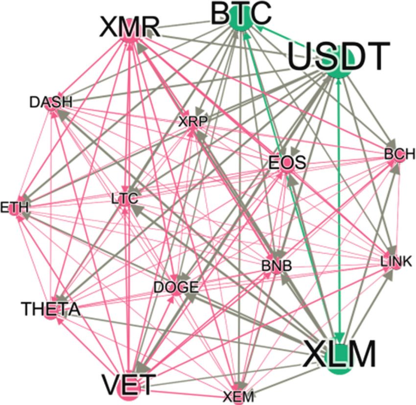
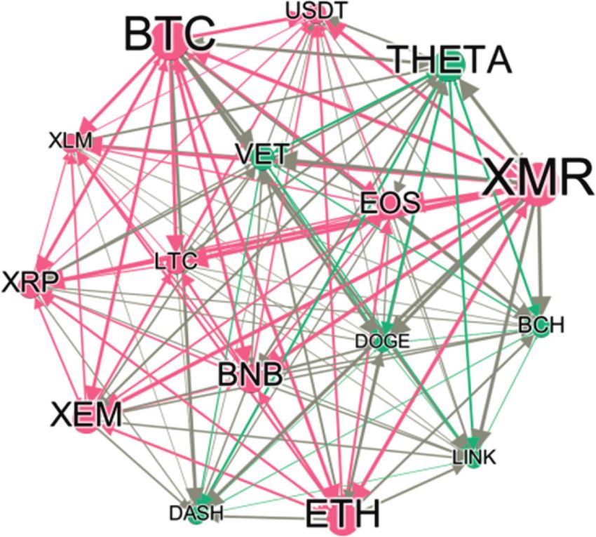
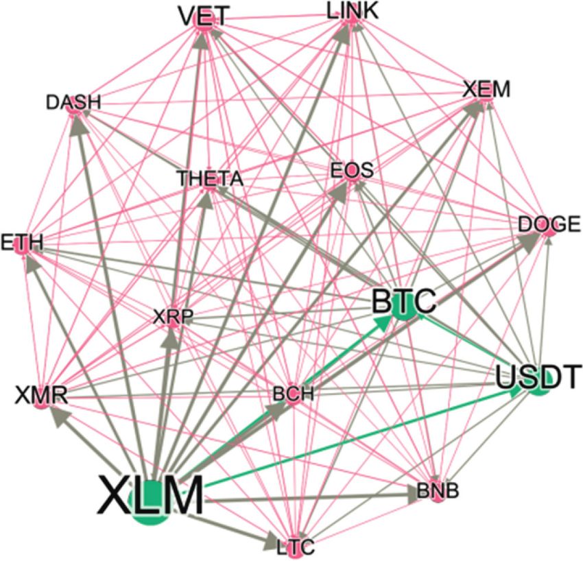
Complexity 7

 Table 2: The dominance of 16 cryptocurrencies. It can be found that under the wavelet packet decomposi-
 tion, the causal relationship between cryptocurrencies is
Name Dominance (%) Price indeed different from that under the original sequence.
BTC 51.76 $58277 Figures 2–6 are more red in the overall picture, while
ETH 12.28 $2210.15 Figures 7–9 are mostly blue, representing the long-term and
BNB 3.67 $497.21 medium-term and short-term, respectively. At the same
XRP 3.16 $1.44728
 time, it can be seen that the long-term gradual change to red
USDT 2.27 $0.997
DOGE 1.76 $0.279866
 is represented in Figures 2–4, there was a gradual change to
LTC 0.9 $277.494 blue in the short term in Figures 7–9, in the medium term
BCH 0.84 $941.27 shown in Figures 5 and 6, we have two extreme colors, nearly
LINK 0.75 $37.41 wholly red or blue, and the medium term may be the key to
VET 0.67 $0.212868 change.
XLM 0.62 $0.56744 In view of the multiple surges of Bitcoin from 2018 to
THETA 0.60 $12.6065 2020, and the first surge of Dogecoin in April 2021, it is
EOS 0.34 $7.4078 particularly important to analyze the causality of a single
XMR 0.28 $335.046 cryptocurrency at different frequencies, as shown in
XEM 0.18 $0.42454 Figures 10–25, respectively. These 16 graphs show the
DASH 0.16 $329.25
 nonlinear relationship between market value and risk, which
The above ranking ends on April 11, 2021, and all data comes from investing fits the previous conclusions. We can see that D8 rows in
website.
 these graphs are more or less blue, even for BTC, which
 occupies the top market. At any frequencies, the three
and then use wavelet packet decomposition to obtain 8 cryptocurrencies (BTC, ETH, and XRP) occupying the main
frequencies under the two-level tree branch. With the market capitalization are almost completely red, that is, the
combination of single rate of return and the market index same strong risk causality for different currencies at different
combination, it is denoted as D8, D7, D6, D5, D4, D3, D2, frequencies. However, in currencies with a relatively small
D1, which express the frequency from 2j to 2j+1 , repre- market value, there is also a strong causal relationship at
senting 2–4, 4–8, 8–16, 16–32, 32–64, 64–128, 128–256, and certain frequency, such as EOS, XMR, and DASH. It can be
256–512 days [43, 81]. Then, using the COVAR-GARCH seen that for the risk contagion of cryptocurrency, the
model (Xu et al. discussed that this method is effective) [82], dominant cryptocurrency, and altcoins also play an im-
the systemic risk of 16 cryptocurrencies at 8 frequencies are portant role, but the conversion relationship among them
obtained which is basic data in the DY matrix and STVAR seems a little vague, and further analysis is needed, which
models, and the one of nonlinear Granger causality test is the provides the possibility for the analysis of the risk contagion
logarithmic rate of return. path of the network. In connection with the multiple surges
 of Dogecoin in April, the causality diagram (Figure 22)
 shows a little trace, that only under D1 the red line appears,
4.1. Nonlinear Granger Causality Test Based on WPT. and the rest are blue. This also provides problem orientation
First, we use nonlinear Granger causality test to make a for expanding systemic risks under time and frequency.
preliminary judgment on the causal relationship between
cryptocurrencies. It has two functions. One is to visually
demonstrate the effectiveness of wavelet packet decompo- 4.2. Risk Spillover Matrix (DY Matrix) Based on WPT.
sition and to verify that the previous frequency analysis First, based on the SC criterion, the optimal lag order for the
results of systemic risks are reliable. The other is to take a VAR basic model is determined to be 2. After the COVAR-
single cryptocurrency as the center, look at its impact under GARCH model is estimated, the “disturbance correlation
different frequencies, and provide a control group for coefficient matrix” (DY matrix) between each crypto-
subsequent determination of frequencies that need to be currency can be obtained, as shown in Tables 4 and 5. We
focused on under different methods. choose D1 and D8 to display, and the results at other fre-
 Table 3 shows the nonlinear Granger causality test be- quencies are available on request. As Tan and Pedersen said,
tween cryptocurrencies under the original sequence. We set the combination of wavelet packet decomposition and
the parameters which embeds dimension at 2 and bandwidth network analysis will greatly improve data performance [68].
at 1 to calculate the causality. The table values are arranged Taking Table 4 as an example, the values at the edges of the
horizontally, taking BTC for instance, and the causal rela- matrix are, respectively, total values, expressing the hori-
tionship between BTC and other currencies is in the second zontal or vertical value of a certain cryptocurrency. The
row, and so on. Due to space limitations, the original data at “TO” column indicates the spillover risk of a certain cur-
other frequencies are available on request. We show it in the rency against other currencies in the market, which is an
form of the heatmap. In the heatmap, the darker the color arrow to go out, and the “FROM” column indicates that
(red), the more significant the causal relationship, and the from the perspective of the total market size, to measure the
lighter the color (blue), the less significant the causal rela- spillover risk of other cryptocurrencies for a certain cur-
tionship. Figures 1–9, respectively, represent the original rency, it is an arrow of entry, which corresponds to the
sequence and the causal relationship at different frequencies. network below, so that the value in the middle of the matrix

8

 Table 3: Nonlinear Granger at original series.
 BTC USDT XLM ETH BNB XEM LTC XRP EOS DASH XMR BCH DOGE VET LINK THETA
BTC −0.595 1.777∗∗ 0.509 1.599∗∗ 0.478 0.842 2.669∗∗∗ 1.625∗ 1.669∗∗ 1.425∗ 0.781 1.655∗∗ 2.028∗∗ 2.442∗∗∗ 2.065∗∗
USDT 0.719 1.057 0.835 2.468∗∗∗ 0.08 2.299∗∗ 1.325∗ 1.894∗∗ 1.545∗ 1.314∗ 2.334∗∗∗ −1.285 −0.644 2.124∗∗ 1.272
XLM 1.324∗ −1.281 −0.227 0.5 2.483∗∗∗ 1.167 2.271∗∗ 0.325 0.863 1.412∗ 0.185 0.692 1.829∗∗ 2.463∗∗ 2.527∗∗∗
ETH 1.495∗ 0.835 1.489∗ 2.768∗∗∗ 0.332 1.609∗ 1.892∗∗ 1.495∗ 2.188∗∗ 2.396∗∗∗ 1.614∗ 1.991∗∗ 1.713∗∗ 3.485∗∗∗ 2.581∗∗∗
BNB 1.182 −0.316 1.497∗ 1.174 1.792∗∗ 1.48∗ 1.65∗∗ 1.969∗∗ 2.911∗∗∗ 1.584∗ 1.733∗∗ 0.249 1.809∗∗ 2.931∗∗∗ 2.495∗∗∗
XEM 0.447 −1.176 1.123 1.136 1.812∗∗ 1.633∗ 1.64∗∗ 0.772 2.196∗∗ −0.118 0.909 1.061 0.628 1.982∗∗ 1.935∗∗
LTC 1.414∗ 0.787 1.274 0.357 1.723∗∗ 0.738 2.041∗∗ 2.574∗∗∗ 1.874∗∗ 1.774∗∗ 2.247∗∗ 2.136∗∗ 1.821∗∗ 2.421∗∗∗ 2.027∗∗
XRP 2.845∗∗∗ −0.209 3.618∗∗∗ 2.344∗∗∗ 2.694∗∗∗ 1.522∗ 2.964∗∗∗ 2.181∗ 2.876∗∗∗ 2.585∗∗∗ 2.452∗∗∗ 1.47∗ 2.749∗∗∗ 2.495∗∗∗ 3.093∗∗∗
EOS 2.429∗∗∗ −0.135 1.853∗∗ 0.619 1.896∗∗ 0.801 3.338∗∗∗ 2.166∗∗ 2.546∗∗∗ 2.632∗∗∗ 2.432∗∗∗ 1.061 2.342∗∗∗ 2.836∗∗∗ 2.704∗∗∗
DASH 2.863∗∗ −1.15 2.321∗ 2.16∗ 3.221∗∗∗ 1.824∗∗ 3.597∗∗∗ 2.236∗∗ 2.891∗∗∗ 3.028∗∗∗ 2.913∗∗∗ 1.843∗∗ 2.614∗∗∗ 3.801∗∗∗ 2.203∗
XMR 2.619∗∗∗ 0.521 2.479∗∗∗ 2.118∗∗∗ 2.701∗∗∗ 1.812∗∗ 2.598∗∗∗ 2.588∗∗∗ 2.056∗∗ 2.108∗∗ 2.385∗∗∗ 0.774 2.31∗∗ 3.487∗∗∗ 2.061∗∗
BCH 0.969 0.254 2.351∗∗∗ 0.892 1.958∗∗ 0.316 2.622∗∗ 2.236∗∗ 1.091 1.718∗∗ 0.915 1.034 1.514∗ 2.983∗∗ 1.726∗∗
DOGE 0.194 −2.771 0.509 0.327 0.314 0.509 0.939 0.622 0.103 0.879 0.895 0.938 1.678∗∗ 1.602∗ 0.58
VET 0.924 −2.704 1.425∗ 0.775 −0.393 1.687∗∗ 1.829∗∗ 2.884∗∗ 0.96 0.82 1.328∗ 1.453∗ 1.149 1.872∗∗ 3.044∗∗∗
LINK 0.968 0.597 1.873∗∗ 1.174 1.866∗∗ 1.036 0.872 1.9∗∗ 1.956∗∗ 1.441∗ 2.045∗∗ 0.308 0.77 0.868 2.595∗∗∗
THETA 1.2 −1.221 1.08 1.011 1.903∗∗ −0.094 1.311∗ 0.721 1.512∗ 1.374∗ 1.195 0.75 0.476 0.646 1.742∗∗
 ∗ ∗∗ ∗∗∗
Note: , , represent the significance tests are passed, respectively, under 10%, 5%, and 1%.
 Complexity

Complexity 9

 3.820 4.420
 THETA THETA
 LINK LINK
 VET VET
 2.500 DOGE 3.140
 DOGE
 BCH BCH
 XMR XMR
 DASH 1.180 DASH 1.860
 EOS EOS
 XRP XRP
 LTC –0.1400 LTC 0.5800
 XEM XEM
 BNB BNB
 ETH ETH –0.7000
 –1.460
 XLM XLM
 USDT USDT
 BTC BTC
 –2.780 –1.980

 BTC
 USDT
 XLM
 ETH
 BNB
 XEM
 LTC
 XRP
 EOS
 DASH

 BCH
 DOGE
 VET
 LINK
 THETA
 XMR
 BTC
 USDT
 XLM
 ETH
 BNB
 XEM
 LTC
 XRP
 EOS
 DASH

 BCH
 DOGE
 VET
 LINK
 THETA
 XMR

 Figure 1: Causality test under Original series9 (D0). Figure 4: Causality test under D3.

 6.820 5.400
 THETA THETA
 LINK LINK
 VET VET
 DOGE 5.212 3.550
 DOGE
 BCH BCH
 XMR XMR
 DASH 3.604 DASH 1.700
 EOS EOS
 XRP XRP
 LTC 1.996 LTC –0.1500
 XEM XEM
 BNB BNB
 ETH 0.3880 ETH –2.000
 XLM XLM
 USDT USDT
 BTC BTC
 –1.220 –3.850
 BTC
 USDT
 XLM
 ETH
 BNB
 XEM
 LTC
 XRP
 EOS
 DASH

 BCH
 DOGE
 VET
 LINK
 THETA

 BTC
 USDT
 XLM
 ETH
 BNB
 XEM
 LTC
 XRP
 EOS
 DASH

 BCH
 DOGE
 VET
 LINK
 THETA
 XMR

 XMR

 Figure 2: Causality test under D1. Figure 5: Causality test under D4.

 7.150 5.400
 THETA THETA
 LINK LINK
 VET VET
 DOGE 4.680 DOGE 3.550
 BCH BCH
 XMR XMR
 DASH 2.210 DASH 1.700
 EOS EOS
 XRP XRP
 LTC –0.2600 LTC –0.1500
 XEM XEM
 BNB BNB
 ETH –2.730 ETH –2.000
 XLM XLM
 USDT USDT
 BTC BTC
 –5.200 –3.850
 BTC
 USDT
 XLM
 ETH
 BNB
 XEM
 LTC
 XRP
 EOS
 DASH

 BCH
 DOGE
 VET
 LINK
 THETA
 XMR

 BTC
 USDT
 XLM
 ETH
 BNB
 XEM
 LTC
 XRP
 EOS
 DASH

 BCH
 DOGE
 VET
 LINK
 THETA
 XMR

 Figure 3: Causality test under D2. Figure 6: Causality test under D5.

10 Complexity

 5.400 6.100
 THETA
 D8
 LINK
 VET D7
 DOGE 3.550 3.760
 BCH D6
 XMR
 DASH 1.700 D5 1.420
 EOS
 XRP D4
 LTC –0.1500 –0.9200
 D3
 XEM
 BNB D2
 ETH –2.000 –3.260
 XLM D1
 USDT
 BTC D0
 –3.850 –5.600
 BTC
 USDT
 XLM
 ETH
 BNB
 XEM
 LTC
 XRP
 EOS
 DASH

 BCH
 DOGE
 VET
 LINK
 THETA
 XMR

 USDT
 XLM
 ETH
 BNB
 XEM
 LTC
 XRP
 EOS
 DASH

 BCH
 DOGE
 VET
 LINK
 THETA
 XMR
 Figure 7: Causality test under D6. Figure 10: BTC to the other.

 5.400 6.100
 THETA
 LINK D8
 VET
 3.550 D7 3.760
 DOGE
 BCH D6
 XMR
 DASH 1.700 D5 1.420
 EOS
 XRP D4
 LTC –0.1500 –0.9200
 D3
 XEM
 BNB D2
 ETH –2.000 –3.260
 XLM D1
 USDT
 BTC D0
 –3.850 –5.600
 BTC
 USDT
 XLM
 ETH
 BNB
 XEM
 LTC
 XRP
 EOS
 DASH

 BCH
 DOGE
 VET
 LINK
 THETA
 XMR

 BTC
 XLM
 ETH
 BNB
 XEM
 LTC
 XRP
 EOS
 DASH

 BCH
 DOGE
 VET
 LINK
 THETA
 XMR

 Figure 8: Causality test under D7. Figure 11: USDT to the other.

 5.400 6.100
 THETA
 D8
 LINK
 VET D7
 3.550 3.760
 DOGE
 BCH D6
 XMR
 DASH 1.700 D5 1.420
 EOS
 D4
 XRP
 LTC –0.1500 D3 –0.9200
 XEM
 BNB D2
 ETH –2.000 –3.260
 XLM D1
 USDT
 D0
 BTC –5.600
 –3.850
 BTC
 USDT
 ETH
 BNB
 XEM
 LTC
 XRP
 EOS
 DASH

 BCH
 DOGE
 VET
 LINK
 THETA
 XMR
 BTC
 USDT
 XLM
 ETH
 BNB
 XEM
 LTC
 XRP
 EOS
 DASH

 BCH
 DOGE
 VET
 LINK
 THETA
 XMR

 Figure 9: Causality test under D8. Figure 12: XLM to the other.

Complexity 11

 6.100 6.100
 D8 D8

 D7 3.760 D7 3.760
 D6 D6

 D5 1.420 D5 1.420

 D4 D4

 D3 –0.9200 –0.9200
 D3

 D2 D2
 –3.260 –3.260
 D1 D1

 D0 D0
 –5.600 –5.600
 BTC
 USDT
 XLM
 BNB
 XEM
 LTC
 XRP
 EOS
 DASH

 BCH
 DOGE
 VET
 LINK
 THETA
 XMR

 BTC
 USDT
 XLM
 ETH
 BNB
 XEM
 XRP
 EOS
 DASH

 BCH
 DOGE
 VET
 LINK
 THETA
 XMR
 Figure 13: ETH to the other. Figure 16: LTC to the other.

 6.100
 6.100
 D8
 D8
 D7 3.760 D7 3.760
 D6
 D6
 D5 1.420 D5 1.420
 D4 D4
 D3 –0.9200 –0.9200
 D3
 D2 D2
 –3.260 –3.260
 D1 D1

 D0 D0
 –5.600 –5.600
 BTC
 USDT
 XLM
 ETH
 XEM
 LTC
 XRP
 EOS
 DASH

 BCH
 DOGE
 VET
 LINK
 THETA

 BTC
 USDT
 XLM
 ETH
 BNB
 XEM
 LTC
 EOS
 DASH

 BCH
 DOGE
 VET
 LINK
 THETA
 XMR

 XMR

 Figure 14: BNB to the other. Figure 17: XRP to the other.

 6.100
 D8 6.100
 D8
 D7
 3.760 D7 3.760
 D6
 D6
 D5 1.420
 D5 1.420
 D4
 D4
 D3 –0.9200
 D3 –0.9200
 D2
 D2
 –3.260
 D1 –3.260
 D1
 D0
 –5.600 D0
 –5.600
 BTC
 USDT
 XLM
 ETH
 BNB
 LTC
 XRP
 EOS
 DASH

 BCH
 DOGE
 VET
 LINK
 THETA
 XMR

 BTC
 USDT
 XLM
 ETH
 BNB
 XEM
 LTC
 XRP
 DASH

 BCH
 DOGE
 VET
 LINK
 THETA
 XMR

 Figure 15: XEM to the other. Figure 18: EOS to the other.

12 Complexity

 6.100 6.100
 D8 D8

 D7 3.760 D7 3.760
 D6 D6
 D5 1.420
 D5 1.420
 D4
 D4
 D3 –0.9200
 D3 –0.9200
 D2
 –3.260 D2
 D1 –3.260
 D1
 D0
 –5.600
 D0
 –5.600
 BTC
 USDT
 XLM
 ETH
 BNB
 XEM
 LTC
 XRP
 EOS

 BCH
 DOGE
 VET
 LINK
 THETA
 XMR

 BTC
 USDT
 XLM
 ETH
 BNB
 XEM
 LTC
 XRP
 EOS
 DASH

 BCH
 VET
 LINK
 THETA
 XMR
 Figure 19: DASH to the other.
 Figure 22: DOGE to the other.

 6.100
 6.100
 D8
 D8
 D7 3.760 D7 3.760
 D6
 D6
 D5 1.420
 D5 1.420
 D4
 D4
 D3 –0.9200
 D3 –0.9200
 D2
 –3.260 D2
 D1
 –3.260
 D1
 D0
 –5.600
 D0
 –5.600
 BTC
 USDT
 XLM
 ETH
 BNB
 XEM
 LTC
 XRP
 EOS
 DASH
 BCH
 DOGE
 VET
 LINK
 THETA

 BTC
 USDT
 XLM
 ETH
 BNB
 XEM
 LTC
 XRP
 EOS
 DASH

 BCH
 DOGE
 LINK
 THETA
 XMR

 Figure 20: XMR to the other.
 Figure 23: VET to the other.

 6.100
 6.100
 D8
 D8
 D7 3.760
 D7 3.760
 D6
 D6
 D5 1.420
 D5 1.420

 D4 D4

 –0.9200 D3 –0.9200
 D3

 D2 D2
 –3.260 –3.260
 D1 D1

 D0 D0
 –5.600 –5.600
 BTC
 USDT
 XLM
 ETH
 BNB
 XEM
 LTC
 XRP
 EOS
 DASH

 BCH
 DOGE
 VET
 THETA
 XMR
 BTC
 USDT
 XLM
 ETH
 BNB
 XEM
 LTC
 XRP
 EOS
 DASH

 DOGE
 VET
 LINK
 THETA
 XMR

 Figure 21: BCH to the other. Figure 24: LINK to the other.

Complexity 13

 6.100
 D8

 D7 3.760
 D6

 D5 1.420

 D4

 D3 –0.9200

 D2
 –3.260
 D1

 D0
 –5.600
 BTC
 USDT
 XLM
 ETH
 BNB
 XEM
 LTC
 XRP
 EOS
 DASH

 BCH
 DOGE
 VET
 LINK
 XMR
 Figure 25: THETA to the other.

 Table 4: DY index under D1.
 BTC USDT XLM ETH BNB XEM LTC XRP EOS DASH XMR BCH DOGE VET LINK THETA FROM
BTC 45.2 4.1 13.9 8.1 5.5 6.4 2.3 1 0.9 0.6 2.1 3.4 1.4 1.7 0.3 3 54.8
USDT 2.5 59.7 5.6 5.8 2.8 1.8 1.8 2.2 0.4 0.5 1.7 1.1 1 5.6 0.3 7.3 40.3
XLM 18 4.1 35.4 7.2 6.6 8.2 3.5 2 2.7 1 3.2 1.6 1.1 1.8 1.9 1.7 64.6
ETH 21 4.3 17.3 20.3 8.1 7.6 2.7 1.2 2.8 1.1 3.4 2 1.6 2.2 1.1 3.1 79.7
BNB 13.9 3.8 13.5 10 35.9 9.8 2.5 0.3 1.4 0.4 3.4 1.6 0.7 0.5 0.9 1.4 64.1
XEM 14.4 2.7 20.5 8.4 5.5 32.2 2 2 1.3 2.2 2.7 0.3 1.3 0.5 1.3 2.7 67.8
LTC 19 4.8 24.1 9.5 7.6 7.8 11.8 1.3 2.4 1 2.6 2 1 2.1 1 1.9 88.2
XRP 15.5 3.2 24 9 6.5 8.9 4.4 14.4 1.7 0.8 3.7 1.5 2.2 1.1 1.1 1.8 85.6
EOS 17.9 3.8 22.1 10.4 8.3 8.4 5.4 1.6 9.1 0.9 3.5 2 1 1.8 1.2 2.6 90.9
DASH 18.5 3.5 20.9 12.4 7.1 8.2 2 1.9 2.8 10.3 3.8 1.1 1.8 1.1 1.2 3.4 89.7
XMR 18.1 4.6 21.1 9.3 8.3 7.6 2.7 2 2.7 2.6 13.1 1.6 1.3 0.9 0.8 3.3 86.9
BCH 20.6 3.1 20.3 12.8 8.3 7.9 3.7 1.5 2.4 2.4 3.4 8.1 1 1.6 0.4 2.6 91.9
DOGE 18.8 3.8 16.2 14 6.7 7.5 3.5 1.2 1.1 0.6 3.9 3 15.6 1.3 0.4 2.6 84.4
VET 17 3.3 19.5 10.9 9.2 9 2.9 5.3 1.3 0.5 2.4 1.3 2 12.5 1.2 1.8 87.5
LINK 14.5 7.3 17.2 13.2 7.2 5.3 1.4 1.3 2.5 1.1 2.6 2.1 1.8 2.9 15.9 3.7 84.1
THETA 19.5 0.1 4.9 0.3 0.1 1.6 1 0.6 0.5 1 1.7 2.5 0.1 0.4 0.2 65.5 34.5
TO 249.2 56.6 261.1 141.4 97.6 106.1 41.7 25.4 26.9 16.8 44.2 27.1 19.3 25.5 13.4 42.9 1195.2
NET 239.6 76 231.9 82 69.4 70.5 −34.7 −45.8 −54.9 −62.6 −29.6 −56.7 −49.5 −49.5 −54.8 73.8 —

 Table 5: DY index under D8.
 BTC USDT XLM ETH BNB XEM LTC XRP EOS DASH XMR BCH DOGE VET LINK THETA FROM
BTC 82.2 3.6 1.5 0.9 1.8 2.4 2.3 0.9 0.1 0 0.5 0.8 1 0.2 0.3 1.5 17.8
USDT 42.4 46.2 1.6 0.2 2.3 1.4 0.8 0.4 0 0 1.3 0.4 1.2 0.1 0 1.7 53.8
XLM 49.4 1.5 37.1 1.8 2.8 0.5 0.7 1.3 0.6 0.2 0.2 0.5 0.8 0.2 0.9 1.3 62.9
ETH 75 3 3.3 7.6 1.7 2 2.2 0.6 0.2 0.1 0.3 0.9 1 0.1 0.4 1.5 92.4
BNB 62.9 4.4 2.5 1.1 21.5 1.1 2 0.9 0 0 0.3 0.5 0.6 0.1 0.1 1.9 78.5
XEM 52.3 2.1 16.8 1.2 2.4 17.2 2 0.2 0.4 0.6 0.2 0.5 1.1 0.4 0.6 2.1 82.8
LTC 66.6 3.2 7.2 2.1 2.3 3.8 10.3 0.5 0.2 0.1 0.1 0.3 0.5 0.2 0.1 2.3 89.7
XRP 54.2 2.2 25.6 0.9 2.5 2.6 1.4 5.2 0.8 0.1 0.3 0.9 1 0.4 0.6 1.3 94.8
EOS 71.6 3.4 4.4 2.6 2.8 1.8 3.4 0.4 5.6 0 0.3 0.6 1.1 0.2 0.2 1.6 94.4
DASH 72.7 3.4 2.7 2.1 1.7 1.7 1.8 1.7 1.3 7.4 0.5 0.7 0.8 0.2 0.2 1.2 92.6
XMR 8.8 22.3 11.8 2.1 2.1 3.3 3.2 0.9 0.4 0.2 41.2 0.2 1 1.4 0.3 0.9 58.8
BCH 54.7 2.3 19.2 2.6 2.6 2.4 1.6 0.4 0.4 0.4 0.4 8.9 0.8 0.3 0.7 2.3 91.1
DOGE 63.4 5.4 2.9 0.6 9.1 0.7 2.1 0.7 0.2 0 0.5 0.3 11.4 0 0.1 2.6 88.6
VET 65.5 4 7.2 1.3 4.8 2.8 1.6 0.6 0.3 0.2 0.4 0.8 0.9 7.7 0.5 1.5 92.3
LINK 59.1 2.9 18.8 2.3 2.2 2 1.9 0.2 0.5 0.3 0.1 0.8 0.9 0.2 6.5 1.1 93.5
THETA 9.1 41.3 0.6 0.2 0.7 0.2 1.4 0.1 0.4 0.2 16.3 0.5 0.2 0.2 0.1 28.6 71.4
TO 807.6 105.1 126 22 41.8 28.7 28.1 10 5.9 2.5 21.8 8.6 12.8 4.5 5.3 24.6 1255.4
NET 871.9 97.4 100.2 −62.7 −15.2 −36.8 −51.3 −79.6 −82.9 −82.6 4.2 −73.6 −64.4 −80.1 −81.7 −18.2 —

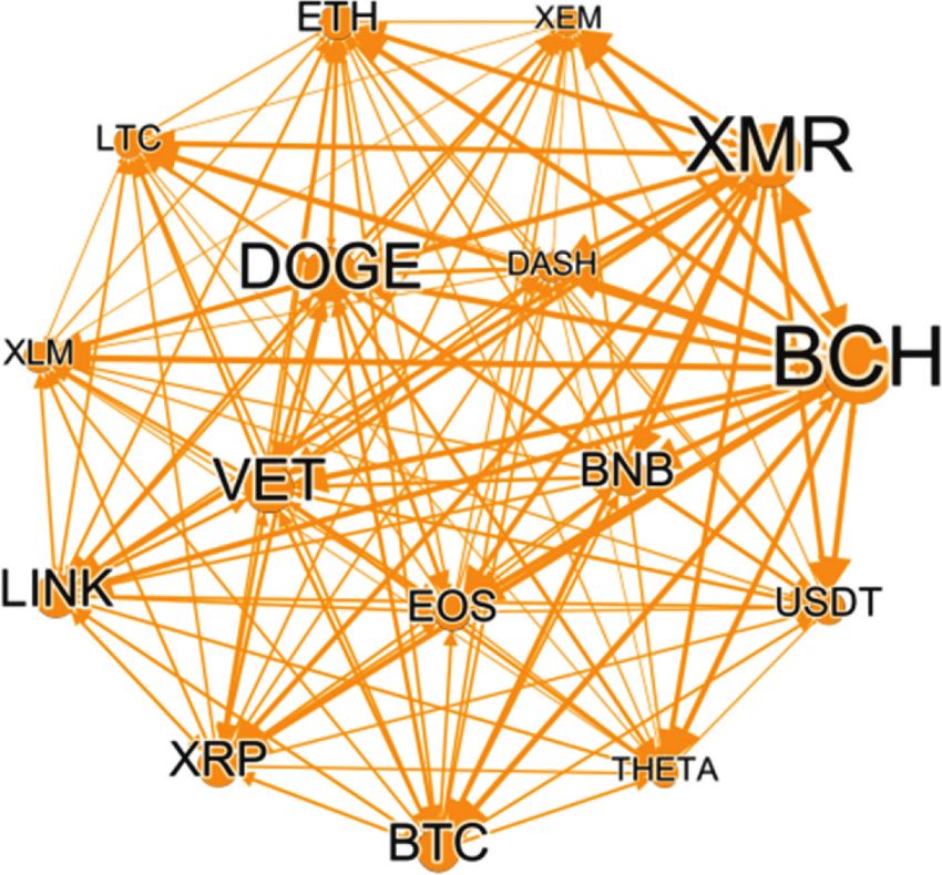
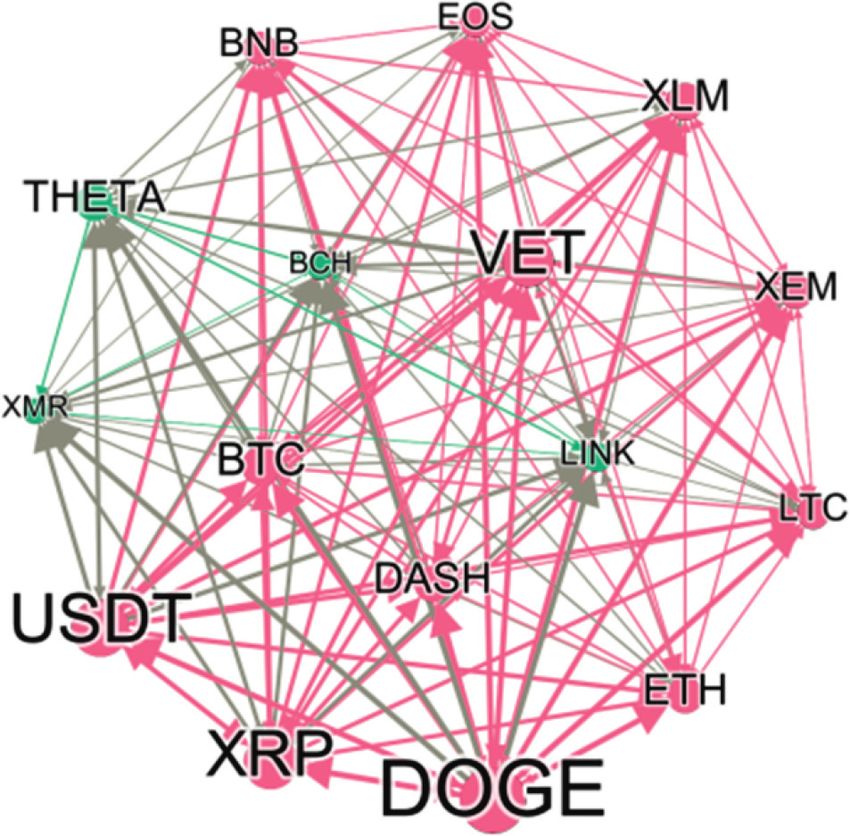
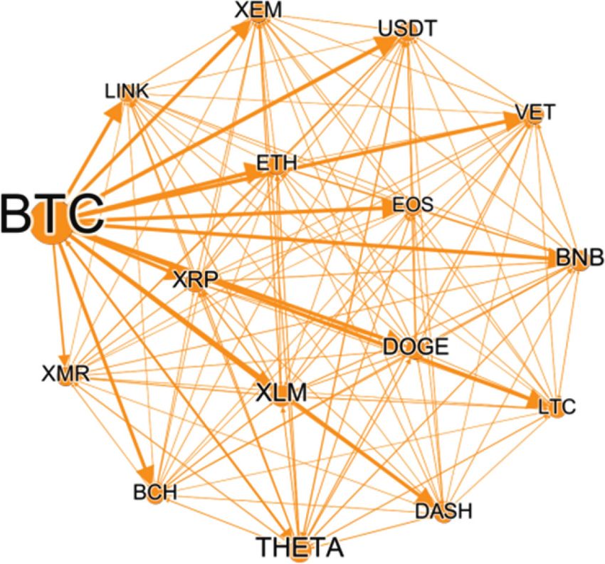
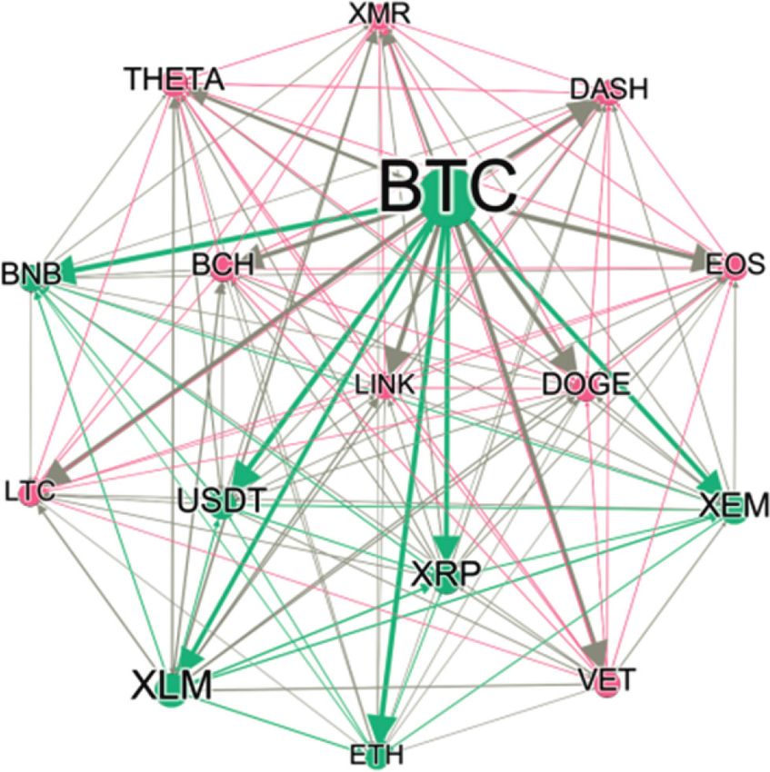
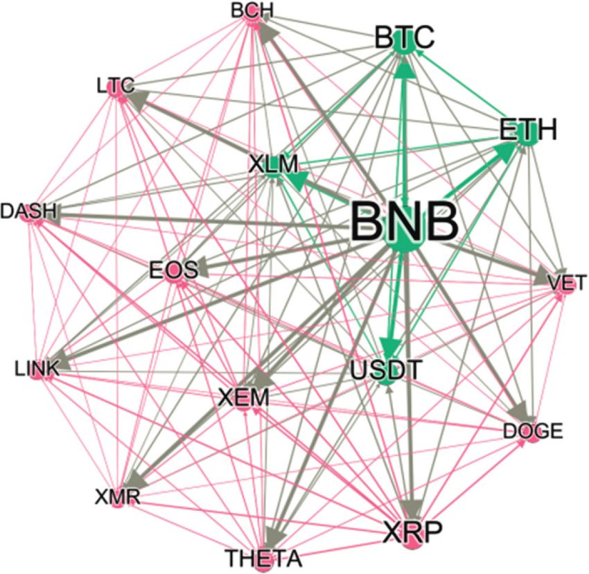
14 Complexity

 Figure 26: Risk spillover under D1.
 Figure 29: Risk spillover under D4.

 Figure 27: Risk spillover under D2.

 Figure 30: Risk spillover under D5.

 Figure 28: Risk spillover under D3.

 Figure 31: Risk spillover under D6.
refers to the risk spillover value between the two. The “NET”
in the bottom row refers to the net spillover effect of a certain
cryptocurrency, that is, the value of the output of the “IN” effect of visible frequency is obvious. Then, we will draw
column offsetting the input of “OUT.” According to the risk networks of risk spillovers at different frequencies, as shown
spillover table, we can see that the net risk spillover intensity in Figures 26–33, to specifically look at the risk infection
on D1 and D8 has dropped from 405% to 345%, and the path between different cryptocurrencies.

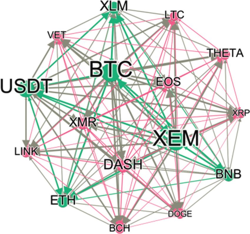
Complexity 15

 cryptocurrencies, which generates risk spillovers, while the
 rest is modular radiation, alongside light power. In the
 following figures, when BTC remains stable, the rest of the
 Bitcoins are also followed behind closely. In the long run, at
 D1, XLM and BTC have reached the point where they resist
 courtesy, while at D3, USDT has far surpassed BTC, ac-
 companying rapid changes. In the mid-term, at D5, BCH
 surpassed BTC, with a strong risk of spilling infection to
 BTC, and at the same time radiating to other crypto-
 currencies with modularity. In the short term, at D6, BNB
 and BTC have the same strong risk spillover. For these
 cryptocurrencies that are about to approach or have become
 risk centers at different frequencies, the risk center changes
 of XLM, BCH, and USDT (Figures 11, 12, and 21) have a
 strong correlation with causality, while BNB is abnormal
 Figure 32: Risk spillover under D7. (Figure 14). At high frequencies, the causality diagram is
 light blue, which is a weaker causality, but under the DY
 matrix, it becomes the risk spillover center in D6. However,
 BCH is a comprehensive red in the causality diagram, with a
 very strong causal relationship, but it only becomes the
 center at D5, and the other frequencies have very little in-
 fluence. This provides a basis for further research on non-
 linear systemic risks.

 4.3. STVAR Model Based on WPT. In order to ensure that the
 introduction of periodicity is theoretically reasonable, we
 conduct a nonlinear test before STVAR model estimation.
 We use BDS test [68], Quandt–Andrews test [83, 84], and
 Bai–Perron test [85] to test the stability of model parameters.
 Among them, the Quandt–Andrews test is the unknown
 mutation point test, and the Bai–Perron test is the multiple
 mutations in the unknown inspection. Table 6 shows the
 results of the parameter stability of the systemic risk eval-
 Figure 33: Risk spillover under D8. uation of each cryptocurrency. For the BDS test, when the
 nesting dimensions are 3, 4, and 5, the null hypothesis of
 independent and identical distribution is significantly
 The risk infection network consists of nodes and edges rejected, indicating that there is a nonlinear relationship
with arrows. The size of the node is set according to the between the variables; that is, it has the characteristic of
weighted-out degree, that is, the net risk spillover repre- being transformable [86, 87]. The mutation point test in-
sented by the NET column value of spillover matrix (Table 4) dicates that the parameters of the model contain one or more
as the weight. The larger the net overflow, the larger the mutation points, which means that the use of constant
node. The color of the node is colored according to the parameter estimation methods will lead to biased model
“modularity” value in the “Gephi” statistical attribute, which estimation results.
means that the similarity of the risk value between different Based on the partial conflict between the above-
cryptocurrencies shows the same community attribute, and mentioned causality and the risk spillover network, we re-
the color of the edge also changes accordingly. The size of the issue the STVAR model to further explore the risk spillover
edge is expressed as the weight based on the intermediate of different states under the same frequency. The highlight of
value of the spillover matrix (Table 4), that is, the degree of the STVAR model lies in the state variable CRIX, which is
risk spillover between the two. On the whole, the risk different from the DY matrix. We use HP filtering
spillover of BTC in the medium and long term is relatively (Hodrick–Prescott filter) to extract the period term of the
stable, except for D7, which is affected by the same modular market index, and the conversion of state variables will
spillover of XLM. The modularity of these frequencies always divide the original data into upward and downward inter-
changes, but the big picture remains consistent in the long vals, that is, expansion and recession. In addition, in the
term (D1-D3), just like that the internal spillover of the first STVAR model, we take the forecast period as 60 periods. The
two intervals are maintained, and the latter is more entering, following data takes the 60th period as an example (we have
which is affected by USDT. But when the frequency is in the observed the risk spillover centers of periods 4, 8, 16, 32, and
mid-term (D4) and the shortest term (D8), BTC becomes the 60, respectively, and they are all consistent. The results are
only module by itself, with a strong spillover effect on other available on request). The result of the variance

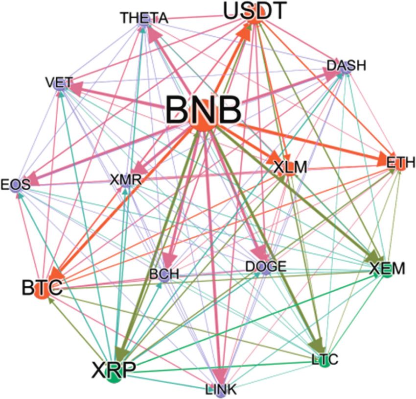
16 Complexity

 Table 6: Mutation point test at D1.
 BDS test at D1 Quandt–Andrews test at D1 Bai–Perron test at D1
Dimension Z-statistic Statistic Value Breaks Weighted F-statistic
2 35.87334∗∗∗ Max LR 27.27269∗∗∗ 1 145.1847∗∗∗
3 36.20612∗∗∗ Max Wald 436.3631∗∗∗ 2 434.7727∗∗∗
4 36.53463∗∗∗ Exp LR 11.24758∗∗∗ 3 582.5047∗∗∗
5 37.66492∗∗∗ Exp Wald 212.3472∗∗∗ 4 634.7938∗∗∗
6 39.70935∗∗∗ Ave LR 14.25429∗∗∗ 5 702.3262∗∗∗
 Ave Wald 228.0686∗∗∗
 BDS test at D8 Quandt–Andrews test at D8 Bai–Perron test at D8
Dimension Z-statistic Statistic Value Breaks Weighted F-statistic
2 26.60005∗∗∗ Max LR 29.01095∗∗∗ 1 464.1752∗∗∗
3 27.80135∗∗∗ Max Wald 464.1752∗∗∗ 2 477.6903∗∗∗
4 29.49901∗∗∗ Exp LR 12.44368∗∗∗ 3 518.6559∗∗∗
5 31.52829∗∗∗ Exp Wald 227.7935∗∗∗ 4 567.7082∗∗∗
6 33.63134∗∗∗ Ave LR 18.9412∗∗∗ 5 582.9202∗∗∗
 Ave Wald 303.0592∗∗∗
Notes: (1) BDS test is based on the residual series. (2) Bai–Perron test is measured at “Global L breaks versus none” and the maximum mutation points set at
Eviews10 is 5.

decomposition results in a superposition of decimal points
and cannot be listed in a limited page. Therefore, we only Table 7: Variance decomposition under D1 and D8.
show the data of the two states of BTC at the frequency of D1 E1 R1 E8 R8
and D8, that is, risk spillover for other cryptocurrencies BTC 0.031598862 0.331499371 0.162869273 0.367568582
(including itself )), as shown in Table 7. USDT 0.022759805 0.322926561 0.159920324 0.360501403
 The following shows the risk spillover network in XLM 0.029465532 0.299483116 0.129024966 0.304571259
different states (regimes) at different frequencies, and its ETH 0.03334609 0.291689594 0.154070093 0.354073605
specific properties are the same as the above network di- BNB 0.027358849 0.320791552 0.146497214 0.351841821
agram. On the whole, under different regimes, the risk XEM 0.02700427 0.29718005 0.136677786 0.318404742
center may change, or the risk intensity may change. Under LTC 0.030847272 0.307208371 0.146460891 0.338103864
D1, BTC is the center of risk in expansion, followed by 5 XRP 0.029534455 0.294918714 0.137492015 0.321451507
 EOS 0.030994604 0.285515889 0.150972283 0.353127934
currencies with different net risk spillover including XLM
 DASH 0.030571503 0.292677478 0.144059299 0.344757499
and XEM in Figure 26, while in recession, only BTC is the XMR 0.029445069 0.310724834 0.078361147 0.173421102
center, and nothing followed. Comparing to the DY matrix, BCH 0.029513472 0.313196399 0.133429574 0.312831387
its comprehensive risk module will remain consistent. DOGE 0.030496163 0.289546516 0.144039877 0.347102666
Under D2, it is in sharp contrast with the DY matrix. The VET 0.029977661 0.305307092 0.147001788 0.343447659
former is the dominant BTC, but at this time, there are LINK 0.027388662 0.304459542 0.139891139 0.327138017
multiple risk centers in both regimes. In recession, the risk THETA 0.029643945 0.322797859 0.087202167 0.235510653
centers not only become DASH and XMR, but BTC only
has minimal net risk spillover. Under D3, USDT exists in
the risk centers of both, which is consistent with the DY expansion is consistent with the DY matrix, while the
matrix. In recession, we can see that DOGE has even be- recession allows USDT increasing. Under D8, XLM re-
come a risk spillover center that surpasses USDT, which places BTC as the center in expansion. Fousekis and Tzaferi
echoes the red and blue causality diagram (Figure 22). believe that returns are more likely to have a fundamental
Under D4, when the risk spillover center maintained the change in causality [88], and the systemic risk of network
foundation of BTC, XMR gradually became stronger, until differs. This may be the explanation.
in recession, surpassing BTC became the only one. Under In the abovementioned, all figures of different regimes
D5, the original degree of risk spillover under DY matrix is under different frequencies are shown from Figures 34–49;
magnified. In recession, DOGE becomes an important besides, the previously emerging BCH, USDT, and BNB,
force for shocking risk. Compared with the center, XMR is even XEM and XMR occupying a small market value can
more significant in recession, and XRP is more significant become the center of risk spillover. On the whole, the
in expansion. The difference is that the modularity effect conclusion that BTC, as a risk spillover center, is more
has disappeared; thus the attributes shown by different credible, but it is also necessary to consider the possibility of
cryptocurrencies show the characteristics of homogeneity. different frequencies and regimes; that is, BTC has strong
Under D6, the risk spillover effect of BTC seems to be risk spillover in the longest (D1) and shortest (D8) periods,
weakened, and BNB occupies the center position. At the and it will be more robust in expansion. For other small
same time, when transitioning from R to E, the modula- cryptocurrencies, medium-term holdings and recession
rization is increased to 3 layers. The increase in modularity periods will be more stable. When examining the changes
has impacted BTC’s risk center position. Under D7, the between different regimes, even DOGE, whose causality is