Readdressing the Trade Effect of the Euro: Allowing for Currency Misalignment - Dis cus si on Paper No. 10-023 Jan Hogrefe, Benjamin Jung, and ...
←
→
Page content transcription
If your browser does not render page correctly, please read the page content below
Discussion Paper No. 10-023

   Readdressing the Trade Effect
            of the Euro:
Allowing for Currency Misalignment
Jan Hogrefe, Benjamin Jung, and Wilhelm Kohler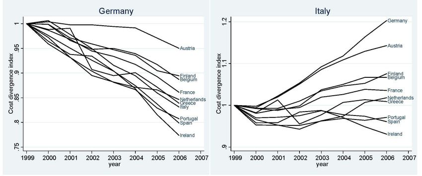
Discussion Paper No. 10-023

                 Readdressing the Trade Effect
                          of the Euro:
              Allowing for Currency Misalignment
             Jan Hogrefe, Benjamin Jung, and Wilhelm Kohler

                    Download this ZEW Discussion Paper from our ftp server:

                ftp://ftp.zew.de/pub/zew-docs/dp/dp10023.pdf

           Die Discussion Papers dienen einer möglichst schnellen Verbreitung von
      neueren Forschungsarbeiten des ZEW. Die Beiträge liegen in alleiniger Verantwortung
          der Autoren und stellen nicht notwendigerweise die Meinung des ZEW dar.

   Discussion Papers are intended to make results of ZEW research promptly available to other
economists in order to encourage discussion and suggestions for revisions. The authors are solely
     responsible for the contents which do not necessarily represent the opinion of the ZEW.
Non-technical Summary
The run-up to the Economic and Monetary Union (EMU) of the EU has been dominated
by tension between a big aspiration and a big concern. The aspiration was that a common
currency would reinvigorate the single market program by establishing more cross-country
transparency, wiping out all exchange rate uncertainty, and lowering administrative cost
of intra-European trade. Euro members were hoping for a significant rise in bilateral trade
generating sizable welfare gains across the currency union.
The concern was that some member countries might face problems in absorbing shocks
in ways that are consistent with a common anchor. Absent nominal exchange rate adjust-
ment within the union, this would result in misalignments of real exchange rates and, thus,
diverging competitiveness. Such misalignments have a trade effect that is of a different
nature compared to the one triggered by a reduction in trade costs, as usually expected
from a common currency. Lower trade costs affect countries in symmetric fashion, raising
all countries exports and imports. In contrast, misalignment-induced trade effects are
asymmetric, whereby bilateral exports and imports deviate in opposite direction from the
benchmark case where bilateral purchasing power is maintained. In short, misalignments
introduce a drifting apart of intra-euro area trade balances. The welfare implications are
different, too. Higher exports from lower trade costs clearly indicate higher gains from
trade. The same is not true, however, if higher exports reflect a deterioration of the terms
of trade, as with a currency misalignment.
In this paper, we use gravity methods to test whether this type of implicit currency
misalignment has had a statistically significant impact on bilateral intra-euro area ex-
ports. We first extend the traditional gravity model to incorporate nominal exchange
rates. A currency union may then raise the hypothetical “gravity-norm-level” of trade
between member states, but may also cause misalignment-induced deviations from this
norm. Guided by our extended gravity model, we then conduct a thorough empirical
assessment of these two effects, using state-of-the art econometric methods. We find that
the introduction of the euro has had a significant currency misalignment effect. The
numbers tell us that an increase in relative nominal unit labour costs by 10% leads to a
7% reduction in exports, if membership in the euro area rules out nominal exchange rate
adjustment, but leaves exports unaffected for country pairs with different currencies with
flexible exchange rates. Given that euro members show diverging patterns of cost com-
petitiveness, being part of the euro area - judged from the trade effects - means different
things for different countries. For instance, we find Germany and Austria to benefit from
the common nominal anchor in terms of higher export volumes. In contrast, for coun-
tries like Portugal, Ireland and Greece, using the euro has had the opposite effect. Wecalculate summary measures highlighting these asymmetries that have so far escaped all attention in the literature. Our results have important implications for overall euro area macroeconomic developments. If there is a trend of competitiveness divergence in euro area trade balances, we might also expect countries to have different outlooks regarding the stability of current account deficits and the amount of external debt. In summary, the hopes might only come true for some, while others will remember the concerns.
Das Wichtigste in Kürze

Im Vorfeld der Europäischen Wirtschafts- und Währungsunion (EWWU) dominierte eine
Abwägung von Hoffnungen und Zweifeln die politische sowie ökonomische Diskussion. Die
Hoffnungen ruhten darauf, dass der Euro dem europäischen Binnenmarkt neuen Schwung
verleihen könnte, indem er die Transparenz zwischen den Mitgliedsländern erhöht, Wech-
selkursunsicherheiten beendet und administrative Kosten für Firmen verringert. Als
Konsequenz hofften die Euroländer auf eine substanzielle Handelsteigerung - mit allen
verbundenen Wohlsfahrteffekten. Die Zweifel bezogen sich darauf, dass manche Länder
wohlmöglich Schwierigkeiten haben würden, makroökonomische Schocks im Einklang mit
einem System fixer Wechselkurs zu absorbieren. Ohne die Anpassung nominaler Wech-
selkurse resultieren daraus Ungleichgewichte der realen Wechselkurse und damit auch Ver-
schiebungen der relativen Wettbewerbsfähigkeit. Solche Ungleichgewichte haben andere
Handelseffekte als die Auswirkungen einer Handelskostenreduzierung, wie sie normaler-
weise von einer Währungsunion zu erwarten sind. Von allgemeinen Handelskostenreduk-
tionen profitieren alle Länder gleichermaßen durch steigende Importe und Exporte. Im
Gegensatz dazu wirken Währungsungleichgewichte asymmetrisch und treiben Importe
und Exporte in unterschiedliche Richtungen gegenüber einer Situation, in welcher die
Wechselkurse den Kaufkraftparitäten entsprechen. Damit treiben implizite Währungsun-
gleichgewichte einen Keil zwischen die Leitungsbilanzen der Euromitglieder. Auch die
Wohlsfahrtseffekte sind andere. Höhere Exporte als Konsequenz sinkender Handelskosten
haben einen klar wohlfahrtssteigernden Effekt. Dies gilt jedoch nicht eindeutig für den
Fall impliziter Währungsungleichgewichte, in dem eine Exportsteigerung mit einer Ver-
schlechterung des Realaustauschverhältnisses (terms of trade) einhergeht.
    In der vorliegenden Studie verwenden wir auf Gravitationsgleichungen basierende
Methoden und testen, ob die angesprochenen impliziten Währungsungleichgewichte in der
Eurozone einen statistisch signifikanten Effekt auf die Handelsströme ausüben. Zuerst
erweitern wir das traditionelle Gravitationsmodell um nominale Wechselkurse. Im er-
weiterten Modell führt eine Währungsunion zum einen zu einer Erhöhung des Han-
dels gemäß einer "Gravitations-Norm", zum anderen entstehen Abweichungen von dieser
Norm, verursacht durch implizite Währungsungleichgewichte. Ausgehend von unseren
theoretischen Überlegungen führen wir eine tiefgreifende empirische Untersuchung der
zwei Effekte auf Grundlage aktuellster Methodik durch. Wir bestätigen, dass der Euro
einen Handelseffekt über den Kanal der Währungsungleichgewichte hat. In Zahlen aus-
gedrückt ergibt sich folgendes Bild: Ein relativer Anstieg der Lohnstückkosten in einem
Land um 10% führt zu einer Exportreduktion um etwa 7%, wenn dieser nicht durch
nominale Wechselkursbewegungen ausgeglichen werden kann. Da in der Eurozone sicht-
bare Unterschiede bezüglich der Wettbewerbsfähigkeit vorherrschen, ergibt sich daraus
ein uneinheitlicher Gesamteffekt des Euro auf den Außenhandel der Mitgliedsstaaten.
Insbesondere profitieren Deutschland und Österreich von festen Wechselkursen, während
sich für Länder wie Irland, Portugal oder Griechenland ein Nachteil einstellt. Wir errech-
nen zusammenfassende Maßzahlen, um die gemessene Heterogenität abzubilden, die sich
bisher jeder Aufmerksamkeit in der Literatur entzogen hat.
Unsere Ergebnisse haben große Bedeutung für makroökonomische Entwicklungen in
Europa. Wenn es einen Trend hin zu verstärkt unterschiedlichen Handelsmustern inner-
halb der Eurozone gibt, können wir auch auf unterschiedliche Aussichten bezüglich der
länderspezifischen Stabilität in den Leistungsbilanzen und der Auslandsverschuldungen
schließen. Zusammenfassen lässt sich festhalten, dass sich die in den Euro gesetzten Hoff-
nungen nur für manche Länder zu erfüllen scheinen. Andere werden sich an die Zweifel
erinnern.Readdressing the Trade Effect of the Euro:
Allowing for Currency Misalignment ∗
†
Jan Hogrefe Benjamin Jung‡ Wilhelm Kohler§
ZEW Mannheim Tübingen University Tübingen University
CESifo and GEP
April 2010
Abstract
We know that euro-area member countries have absorbed asymmetric shocks
in ways that are inconsistent with a common nominal anchor. Based on a
reformulation of the gravity model that allows for such bilateral misalignment,
we disentangle the conventional trade cost channel and trade effects deriving
from “implicit currency misalignment”. Econometric estimation reveals that
the currency misalignment channel exerts a significant trade effect on bilateral
exports. We retrieve country specific estimates of the euro effect on trade based
on misalignment. This reveals asymmetric trade effects and heterogeneous
outlooks across countries for the costs and benefits from adopting the euro.
JEL Codes: F12, F13, F15
Keywords: Euro, gravity model, exchange rates, purchasing power parity, trade
imbalances
∗
We would like to thank Andreas Sachs and workshop participants at Hohenheim University,
Göttingen University, ZEW Mannheim and the SMYE 2010 in Luxembourg for valuable comments.
The views expressed in this paper are solely those of the authors. All possible errors are, of course,
ours as well.
†
Centre for European Economic Research (ZEW), P.O. Box 103443, D-68034 Mannheim, Ger-
many. Email: hogrefe@zew.de
‡
Tübingen University, Nauklerstrasse 47, D-72074 Tübingen, Germany. Email:
benjamin.jung@uni-tuebingen.de
§
Tübingen University, CESifo and GEP, Nauklerstrasse 47, D-72074 Tübingen, Germany.
Email: wilhelm.kohler@uni-tuebingen.de1 Introduction
The run-up to the Economic and Monetary Union (EMU) of the EU has been dom-
inated by tension between a big aspiration and a big concern. The aspiration was
that a common currency would reinvigorate the single market programme by estab-
lishing more cross-country transparency, wiping out all exchange rate uncertainty,
and lowering administrative cost of intra-European trade. The concern was that
some member countries might face problems in adjusting to a common nominal an-
chor. In order to allay fears of macroeconomic instability that would possibly result
from such problems, ex ante macroeconomic convergence was installed as a prereq-
uisite for membership in the currency union. The famous Maastricht entry criteria
were supposed to guarantee, or at least foster, the ability of all member countries
to live with a stable common nominal anchor ex post. In addition, the Stability
and Growth Pact (SGP) has installed a rule of conduct, in order to ensure that the
stability of this anchor would not be jeopardised from member countries’ waning
fiscal discipline.
Ten years on, we now have a wealth of evidence to judge whether the aspirations
have been met and the concerns have been justified. On the macroeconomic side, the
verdict seems split. On the one hand, the success of the Euro system in establishing
lasting stability of the nominal anchor seems beyond doubt; see Wyplosz (2006). On
the other hand, member countries’ longer-term abilities to live with this anchor in
some cases are in doubt, judged from the build-up of public sector imbalances, as
well as from responses of nominal wage levels to country-specific shocks, which have
lead to sizable misalignments of real exchange rates, as detailed in a recent report
by the European Commission.1
On the single market aspirations, the verdict might draw on evidence of a trade-
enhancing effect of the euro. While the famous tripling estimate which Rose (2000)
found for pre-euro currency unions could never be reestablished for the euro area,
the literature has produced a host of studies confirming positive effects on bilateral
trade for the euro area as well. Early studies found effects around 15%, while more
recent estimates based on refined econometric techniques reveal an effect barely
above zero, if any at all; see Baldwin et al. (2008).
Setting overarching “European ambitions” such as the single market aspirations
aside, a significant trade effect may seem like a necessary benefit to justify the cost
1
See Volume 8 N◦ 1 (2009) of the Quarterly Report on the Euro Area.
1of euro membership. After all, for several countries satisfying the relatively strong
ex ante convergence criteria was quite costly, without any clear evidence of a lasting
benefit, other than being part of the Euro; see Wyplosz (2006). Nor has the pain
necessarily gone after entry. Member countries are subject to rigorous surveillance
from Brussels and compliance with potentially painful fiscal rules under the Stability
and Growth Pact. Furthermore, euro members delegate all monetary policy control
to the European Central Bank, for the sake of a common nominal anchor that does
not equally suit each individual member. Arguably, where countries are willing
to pay such a price, there should also be a benefit. For most countries, a large
enough boost in trade, due to higher transparency, lower uncertainty, and lower
administrative cost, would conceivably be worth paying the price.2
In this paper, we argue that existing estimates of the trade effect of common
currencies, particularly of the euro, suffer from ignoring what we call the currency
misalignment channel. In most cases, the framework adopted involves estimation
of the gravity model of bilateral trade, allowing for a common currency to affect
bilateral trade through the so-called trade cost channel. This seems like an obvi-
ous approach, since it allows to conveniently control for determinants of bilateral
trade other than a common currency, and to infer the magnitude of a trade effect,
if any, from the coefficient estimate of a common currency dummy. However, such
estimates contain very limited information and are fraught with a serious problem
of interpretation, if the currency union suffers from internal real exchange rate mis-
alignments. In the euro area, such misalignments have been building up in sizable
magnitudes, due to tensions generated by a common nominal anchor in the pres-
ence of asymmetric shocks. We shall present some descriptive evidence on bilateral
misalignments below. It is a safe guess that they have also had a profound impact
on bilateral trade flows. Existing studies ignore this channel. What we need is
an empirical framework that disentangles the trade cost channel and the currency
misalignment channel as two conceptually different ways through which adopting a
common currency affects bilateral trade. This paper proposes and implements such
a framework.
The central contributions of this paper are as follows. First, we reformulate the
2
It must be emphasised that easier and less costly trade generates sizable welfare gains, even if
there is no associated increase in trade volumes. Indeed, alluding to the standard diagrammatical
representation, the “rectangle gains‘” on pre-existing trade volumes are likely to be larger than the
“triangle gains” deriving from a trade volume effect. In a similar vein, Fontagné et al. (2009) argue
that the euro has brought important firm-level gains that need not show up in enhanced aggregate
trade.
2gravity model of bilateral trade with nominal exchange rates and misalignments
within currency unions brought to the fore. An equation of the usual form appears
for what we call the “gravity norm”, i.e., a world that satisfies suitably defined bilat-
eral purchasing power parities between all country pairs. Actual trade volumes then
emerge as deviations from this norm that are caused by within union misalignments.
Based on this model, we develop an empirical framework that allows us to address
the trade cost channel affecting the “gravity norm” levels of bilateral trade, as well as
the misalignment channel causing deviations from the norm. Secondly, within this
framework, we analyse the bias that we must expect to be present in conventional
estimates of trade effects from the euro where the currency misalignment channel
is ignored. We show that these estimates may be interpreted as marginal effects
from the trade cost channel for a hypothetical “sample mean country” that has no
bilateral misalignment. While this seems reassuring for the existing literature, it
masks potentially severe country heterogeneity. We argue that addressing country
heterogeneity in terms of misalignments is very important, because deviations from
the “gravity norm” have welfare implications akin to terms of trade effects. Thus,
they are vastly different from those pertaining to changes in the “gravity norm”. Our
third contribution, therefore, is to bring our framework to euro data, estimating a
currency misalignment coefficient, alongside the conventional trade cost effect, and
to portray a disaggregate picture of how different countries’ trade volumes have been
affected by introducing the euro.
Our approach relies on state of the art estimation of a gravity equation on bilat-
eral merchandise exports, with a common currency dummy capturing the trade cost
channel. However, we additionally allow for a bilateral index of disparity in nominal
unit wage costs to influence bilateral exports. The maintained hypothesis is that
for country pairs that have separate currencies with a “reasonably flexible” nominal
exchange rate, disparity in nominal wage levels should play no role, since nominal
exchange rate adjustments may re-establish bilateral purchasing power. But for euro
members, since such an adjustment is ruled out, nominal wage level disparity should
exert a significant influence on bilateral trade. We estimate this effect through an
interaction of wage disparity and a common currency dummy, a procedure that we
justify through a suitable extension of the gravity model. Our results indicate that
the currency misalignment effect is important and drastically changes conclusions
drawn from conventional estimates in previous studies. In particular, our approach
enables us to address cross-country heterogeneity in the trade effect of the euro. We
decompose the euro effect on trade into the traditional trade cost effect, assumed to
3be common for all countries, and a country-specific misalignment impact.
The paper is structured as follows. In the next section we develop a our argument
for why we should bother about the currency misalignment problem when estimating
trade effects of a common currency in a gravity framework. Subsequently, section
3 further motivates our analysis by showing descriptive evidence on misalignments
in the euro area. Section 4 then develops the extended gravity model where we
explicitly determine nominal factor prices and allow for nominal wage level disparity
to cause a deviation from the “gravity norm”. The model serves as a basis for the
subsequent empirical estimation. Section 5 introduces the empirical framework,
specifying the estimation equation and describing the data. It also presents the
results. Section 6 concludes the paper.
2 Why bother about currency misalignments?
Applying the gravity model in the present context amounts to exploiting cross-
country as well as time-variation in exchange rate arrangements and bilateral trade
volumes. This means attempting to see whether trade rises due to countries in-
troducing a common currency, if all other determinants of trade are adequately
controlled for. Correct identification of the true common currency effect using this
approach hinges on the validity of the gravity model of trade and a correct empir-
ical estimation strategy, as well as on successfully controlling for relevant country
heterogeneity. Of course, what we are interested in is the trade effect of the euro,
other things equal. The gravity approach tries to accomplish this by letting other
gravity-type determinants “speak up” in the estimation, leaving for the common
currency dummy to explain variation of bilateral trade across country pairs that
other country characteristics cannot explain. Yet, the standard approach is liable
to yield biased estimates in the presence of unobserved country (or country pair)
heterogeneity, and also if euro membership itself is endogenous, even if all country
heterogeneity is observed.3
Our concern can be framed in terms of country heterogeneity, but of a specific
3
For a general discussion of these problems, see Baier and Bergstrand (2007). An alternative
approach that does not hinge on the validity of the gravity approach to bilateral trade is to pursue
propensity score matching, in order to ensure the “other things equal condition” when comparing
trade across country pairs with and without a common currency; see Persson (2001). Frankel
(2009) uses trade flows from African countries with currencies linked to, first, the French Franc
and later the euro, in order to tackle the endogeneity issue. He confirms a positive trade effect of
the euro.
4type that we argue needs to be put into the foreground, rather than just somehow
be controlled for. It has to do with the trade effects of what, after all, a common
currency is all about, viz. establishing a common nominal anchor between differ-
ent countries. In all likelihood this means different things for different countries,
depending on the shocks, and shock absorption mechanisms, prevailing in different
countries. We argue that the usual gravity-type controls do not capture heterogene-
ity in shock absorption in a satisfactory way.
Consider, first, the question of a selection effect. It is all too obvious from the
Maastricht entry criteria that euro members are no random selection of otherwise
similar countries. The hope was that Maastricht-type convergence ex ante would
somehow guarantee that member countries would eventually establish mechanisms
of shock absorption that are in line with a stable common nominal anchor ex post.
Note that there is some irony here: The very fact that this hope has turned out
illusive can now be argued to question any Maastricht-type selection effect, which
should strengthen the general validity of the gravity estimates of the trade effect.
This is of interest when looking at euro area experience from a broader perspective
of currency union effects, but our concern is a different one.
Suppose, then, that there is no selection effect. What remains is that the trade
effect of euro membership, estimated in the aforementioned way, confounds two fun-
damentally different channels. One is the conventional trade cost channel, which the
gravity approach seems tailored to pick up, and which typically underlies interpre-
tations of the results obtained in the literature. Importantly, this channel operates
symmetrically across all countries. The other is the currency misalignment channel
which – almost by definition – operates asymmetrically. It arises, if some countries
of the union – for whatever reason – experience, or actively pursue, shock absorp-
tion that is inconsistent with the common nominal anchor. In the present context,
perhaps the most important dimension of shock absorption is nominal wage levels.
But why should confounding these two channels cause problems? After all, the
gravity model does not explicitly specify any role of nominal exchange rates or
international currency arrangements. Although researchers typically allude to trade
costs, the approach actually leaves open what it is, exactly, that makes countries
trade more with each other if they share a common currency, compared to a situation
in which they don’t.4 At first sight, this may seem like an advantage in that the
4
The same applies, if one attempts to identify differential trade effects of a richer classification
of currency arrangements that includes varying degrees of exchange rate flexibility. For a study
that implements a classification of 12 degrees of exchange rate flexibility, see Egger (2008).
5approach allows us to pick up any effect that one can possibly imagine.
But for the same reason, a correct interpretation of the estimated effects seems
very hard, or impossible, if both the trade cost and the currency misalignment
channels are operative in the sample. Consider, for instance, the welfare gains.
Arguably, these should provide the ultimate rationale for enhanced trade. Clearly,
enhanced trade that emerges from the trade cost channel and trade effects that derive
from real exchange rate misalignments have different welfare implications. Trade
cost reductions generate the usual “rectangle” and “triangle” gains, symmetrically
for all countries.5 By way of contrast, misalignment-induced trade generates welfare
effects akin to terms of trade effects, which are clearly asymmetric in nature. In view
of the mercantilistic tone that often prevails in popular arguments related to trade
effects of the euro, it is perhaps worth pointing out that an increase in exports due to
a real exchange rate depreciation involves a term of trade deterioration. This seems
a long shot from welfare gains from trade expansion. To summarise this point, any
given trade effect of a common currency will mean very different things, depending
on the presence (or not) of a currency misalignment effect behind trade.
One might argue that, since any currency misalignment by definition is a bilat-
eral affair of over- and undervaluation, misalignment effects should cancel out in the
overall picture. Accordingly, they should not harm aggregate estimates of the trade
cost effects too much. One might question this argument on empirical grounds, since
misalignment effects should still be expected to affect aggregate trade, if countries
are of unequal size, or if bilateral trade is unbalanced. We shall demonstrate below
that within our empirical framework – somewhat surprisingly – the conventional
procedure does indeed generate unbiased estimates of the marginal trade-cost ef-
fect of a common currency for a hypothetical “sample mean country”. However, it
seems difficult to imagine that one would be satisfied knowing the aggregate trade
cost effect, recognizing that it masks significant country heterogeneity from multiple
misalignments within the currency union. There is no way to avoid the conclusion
5
Note that even pure trade cost channel effects are but an incomplete measure of the welfare
effects from euro-enhanced trade. Specifically, the bulk of gains arise on inframarginal trade. In-
voking a simple partial equilibrium diagram, the estimated trade effect, combined with an estimate
of the price elasticity of trade, would allow us to infer a “price-equivalent effect” of the trade cost
channel effect on trade volumes. It is then straightforward from the usual partial equilibrium ex-
position to calculate the “triangular” welfare increase from trade expansion. But more importantly,
the “rectangle” gains then follow from the price-equivalent effect and the pre-existing, inframarginal
volume of trade. In addition to the traditional effects, there are variety and scale effects suggested
by new trade theory, as well as productivity effects from firm heterogeneity stressed by the “new
new” trade theory.
6that the currency misalignment channel needs appropriate attention in the empirical
analysis. Therefore, we now proceed to a suitable reformulation of the gravity ap-
proach leading to an empirical framework that allows us to do so, and to implement
this framework towards a disaggregate, country-specific view on the trade effects of
the euro.
3 Descriptive evidence on misalignment
Before we proceed with a refinement of gravity-modeling and estimation, we take a
quick look at the data in order to see whether we are talking about a phenomenon
of empirical importance. In terms of the model developed in the next section,
we calculate bilateral measures of cost divergence as m̄ijt = c(wit )/c(wjt ), where
w.t denotes a vector of nominal factor prices (e.g., wages) prevailing in euro area
countries i and j, respectively, at time t, and c(·) denotes a minimum unit-cost
function for aggregate output.6 Considering that within the euro area nominal
exchange rate adjustments are no longer possible, any long-run upward or downward
trend in m̄ijt must be seen as an implicit intra-euro “currency misalignment” in the
sense discussed above and identified precisely in the next section.
We focus on unit labor costs, relying on data from the Organisation for Economic
Cooperation and Development (OECD). These measures, representing the average
cost of labor per unit of output, can be seen as a reflection of a country’s cost
competitiveness.7 Germany and Italy are good cases in point. Figure 1 shows the
values of m̄ijt , where the left-hand panel sets i = Germany and the right-hand
panel sets i = Italy, with j indicating other euro members in either case. We set
the index base-year to 1999, thus assuming that the euro entry exchange rates at
the start were roughly in line with bilateral purchasing power. The figure clearly
shows that the currency misalignment was not a “dead channel” for trade between
the two countries and the other euro area members. Germany has experienced
significant real depreciation vis à vis all other countries, indicating substantial gains
in relative competitiveness. For Italy, the picture is a little less clear cut, but in
6
For ease of exposition, we assume c(·) to be the same for each country. Our empirical strategy
in no way relies on this assumption.
7
Note that competitiveness here is not to be interpreted as fully comprehensive. Changes in the
cost of capital may be considered as well when assessing the overall competitiveness of a country.
However, in the euro area interest rates are set by the ECB for all members while labor market
policies remain within the realm of national governments.
7Figure 1: Unit labor cost relative to other euro-area countries
the majority of cases it has experienced a sizable real appreciation and a loss in
relative competitiveness. In a bilateral trade context, we would then expect exports
from Germany to Italy to rise above, while those from Italy to Germany would fall,
relative to what we will subsequently call the “gravity norm” level of bilateral trade.
Table 1 presents evidence for the rest of the euro area. The values in the first
column refer to averages over all euro area partner countries in the year 2006; the
second column shows the respective values averaged over time since 2000. Note
that in 1999, by definition, there was no misalignment. The table documents a
considerable degree of divergence in bilateral unit labor costs across the euro area.
It can also be seen that for most countries the recent misalignment is larger than
the average value, pointing towards cumulative divergence processes. We conclude
that there is a multiple and varied pattern of bilateral misalignment. Living with
a common nominal anchor has proven less trouble-free ex post than was hoped for
ex ante. In view of the above considerations, this strongly suggests a euro-induced
effect of implicit currency misalignment on bilateral trade that should be taken into
account when estimating the trade effect in a gravity context.
A remaining concern is whether the new currency arrangement indeed stands for
a strong break with the monetary past of the respective countries. In particular, from
a legal perspective, exchange rates where far from a free float under the European
Monetary System (EMS) even before the currency union was formed. However, the
bands within which national currencies were allowed to fluctuate still provided ample
opportunity for exchange rate adjustments, in order to compensate for diverging
8Table 1: Currency misalignment by country
Country (i) 2006 2000-2006
Germany 0.8490 0.9185
Austria 0.8989 0.9323
Finland 0.9610 0.9790
Belgium 0.9699 0.9798
France 1.0021 0.9970
Netherlands 1.0212 1.0397
Greece 1.0312 1.0208
Italy 1.0413 1.0108
Portugal 1.0752 1.0563
Spain 1.0877 1.0408
Ireland 1.1261 1.0545
Note: Averages across countries j.
Annual averages for 2000-2006.
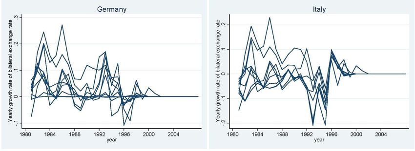
nominal cost conditions. Thus, figure 2 shows that the bands were indeed used in
non-trivial amounts for the various countries’ macroeconomic mechanisms to absorb
asymmetric shocks. The figure depicts yearly log-changes in bilateral exchange rates,
again focusing on Germany and Italy as two obvious cases in point.8
Figure 2: Pre-euro exchange rate movements for Germany and Italy
8
The European Monetary System (EMS)) has allowed nominal exchange rates to fluctuate
within a band of 4.5% in the time from 1979 through 1993. Italy was an exception and was allowed
to widen this band to 6%. Following a massive disruption in 1993, the band was further widened
to 15%. Note also that not all countries in the sample were at all times members of the EMS. In
particular, Austria joined in 1995, Finland in 1996 and Greece in 1998.
94 Currency Misalignment in the Gravity Model
4.1 “Gravity norm”: The trade cost channel
We now turn to a theoretical gravity model in order to formalise our idea of disentan-
gling the trade cost and the currency misalignment channels as two fundamentally
different ways in which introducing the euro as a common currency within the EU
may have affected trade volumes. Suppose we have the usual Dixit-Stiglitz-type
underpinning of the gravity approach. Denoting the c.i.f.-price in country j for a
variety arriving from country i by pij , the quantity of demand Dij for this variety is
Dij = Aj (pij )−σ , (1)
where Aj := Yj (Pj )σ−1 and σ > 1 denotes a uniform elasticity of substitution
between different varieties of goods. In this expression, Yj is equal to country j’s
GDP, and Pj is the exact price index (unit-expenditure function), depending on
prices of all varieties shipped to market j.9 Importantly, all variables on the right-
hand side of (1) are in country j’s currency.
To address the issue of currency misalignment, we now introduce nominal factor
prices. Suppose that in each country there are K primary factors, and assume that
all input use is in terms of the same bundle of primary inputs. We model this
by means of a constant-returns-to-scale function g(v), where v denotes a vector of
factor inputs employed in order to generate the input bundle. More specifically,
we assume that production of a variety requires a fixed amount f and a constant
amount a of this bundle per unit of output. For ease of exposition, we assume
technology to be uniform across all countries, although our results in now way hinge
on this assumption. Unlike Helpman et al. (2008), we assume that all firms have the
same productivity in terms of both marginal and fixed cost. Variable and fixed cost
in any country i then depend on country i’s factor prices wi . Writing c(w) for the
minimum unit-cost function dual to g(v), the cost conditions in domestic currency
are governed by
ci = c (wi ) , (2)
where wi denotes a K ×1 vector of nominal factor prices in country i. The c.i.f.-price
9
In replacing expenditure levels through GDP, we assume total trade to be balanced.
10of a typical variety exported from i to j is then equal to
Tij c (wi ) a
pij = Eij , with ρ := (σ − 1)/ σ (3)
ρ
In this equation, we use Eij to denote the nominal exchange rate, defined as the
price of currency i expressed as in units of currency j. For simplicity, we scale units
such that a = 1.
Arguably, monetary stability over time requires that the purchasing power of
a unit of money over the inputs required to generate a unit of aggregate output
should remain constant. Alternatively, it may be defined as a constant level of the
unit expenditure function. We define a stable nominal anchor as a constant level
of c(w).10 By analogy, we define bilateral purchasing power parity (PPP) between
countries i and j as a situation where both countries have the same nominal cost of
generating the bundle g(v), if expressed in the same currency unit. The PPP level
of the nominal exchange rate, henceforth denoted by Ẽij , is then implicitly defined
through
c (wj )
c wi Ẽij = c (wj ) =⇒ Ẽij = (4)
c (wi )
The second equation uses linear homogeneity of the minimum unit-cost function.
Notice that with C different currencies there are C − 1 independent exchange rates.
If PPP holds between countries i and j, as well as between i and k, then it also
holds for countries j and k.
In what follows, we use .
mij := Eij Ẽij (5)
as the factor of bilateral currency misalignment. If mij = 1 throughout, then there is
no currency misalignment, and Eij c(wi ) = c(wj ). Expressed in a single currency, say
country 1’s currency (e.g., US$), the minimum-unit-cost of the factor bundle g(v)
then is the same world-wide: (Eij Ei1 ) c(wi ) = c(w1 ) for all i and j.11 All possible
countries of origin for any country j’s imports then have the same underlying cost
conditions, governed by real forces like productivity.
10
This captures the idea of a constant purchasing power of money over time, but it avoids
dependence of the nominal anchor on the degree of variety offered in goods markets, which would
arise when using the unit-expenditure function.
11
Bilateral PPP implies that nominal cost in country i, expressed in j-currency is Eij c(wi ) =
c(wj ). It also implies that the nominal cost in country j, expressed in country 1’s currency is
E1j c(wj ) = c(w1 ). Taken together, this implies Eij Ej1 c(wi ) = c(w1 ) for all i and j.
11Thus, for universal PPP, the gravity model of bilateral trade may be written
and estimated without any role for nominal exchange rates, with all prices and
trade values interpreted as being expressed in any one currency, say US$. Due to
zero degree homogeneity of (1) in prices and incomes, the solution of the model
is invariant to the currency in which incomes and prices are expressed, provided
that PPP holds universally. For instance, in the model detailed in Kohler and
Felbermayr (2009), introducing currencies and imposing bilateral PPP would then
tie down c(wi ) for all i to c(w1 ).
In what follows, we call this the “gravity norm”, and we use currency 1 as our
“numéraire currency”. Establishing a currency union affects “gravity norm trade
flows” through the trade cost channel. Empirically, this is captured through a suit-
able specification of Tij . In the sequel we shall indicate hypothetical “gravity norm
values” through a tilde. The “gravity norm” demand function then emerges as
[Pj (T1j c(w1 )/ ρ . . . TCj c(w1 )/ ρ)]σ−1
D̃ij = Ỹj (6)
[Tij c(w1 )/ ρ]σ
−1
[Pj (T1j . . . TCj )]σ−1
c(w1 )
= Ỹj , (7)
ρ (Tij )σ
where Pj (·) denotes the familiar Dixit-Stiglitz-type price index over all varieties
consumed in country j. It should be noted that Ỹj is notional “gravity norm GDP”
of country j, expressed in currency 1. This will in general be different from actual
GDP, also expressed in currency 1.
Anderson and Van Wincoop (2003) have shown that, with symmetric trade costs
Tij = Tji , the usual equilibrium conditions of zero profits (free entry), as well as
goods and factor market clearing, the following equations arise for the value of
aggregate exports from country i to country j:12
!1−σ
Ỹi Ỹj Tij
X̃ij = (8)
Ỹ Π̃i Π̃j
1−σ XC 1−σ
with Π̃j = s̃i Π̃i Tij for i, j = 1, · · · , C (9)
i=1
where si is country i’s share in world-GDP Y . Equations (8) and (9) represent the
12
See Kohler and Felbermayr (2009) for a derivation of a similar equation that takes into account
the so-called extensive country margin, whereby any given exporter does not necessarily serve all
foreign markets.
12full “gravity-norm-solution” of this model. Note that (9) represents a C-dimensional
system of non-linear equations determining the so-called multilateral resistance terms
Π̃j for all countries j = 1, · · · , C as functions of exogenous iceberg trade costs Tij .
Symmetry of trade costs implies that a country’s multilateral trade resistance is the
same on its export and its import side.
4.2 Asymmetric shock and implicit misalignment
Deviations from the “gravity norm” may arise due to asymmetric shocks, or different
shock absorption mechanisms across countries. Consider, for instance, endowment
shocks subject to a downward rigidity of some nominal wage rate. Faced with such
rigidities, countries often follow a strategy of permitting differential increases of
nominal wages and prices, so as to achieve real wage flexibility and, thus, to avoid
unemployment. It is easy to see that this may give rise to misalignment. The K − 1
equilibrium relative factor prices are determined through the following system of
K − 1 equilibrium conditions:
ck (wi ) vik
= for k = 2 . . . K (10)
c1 (wi ) vi1
This simply states that, for all possible factor pairs, the cost-minimising input ra-
tios in production of aggregate output are in line with the corresponding relative
endowments.13 Suppose that the common nominal anchor requires c(w) = 1, and
assume that at time 0 we have c wj0 = c (wi0 ) = 1, with wi0 and wj0 expressed in
common currency, and satisfying equilibrium conditions (10). Moreover, suppose
that countries i and j are hit by asymmetric endowment shocks vi1 − vi0 6= vj1 − vj0 ,
and assume that country j can absorb this through full employment factor prices
wj1 that satisfy c wj1 = 1. A case of misalignment may then arise, if for country i a
change in factor prices that satisfies both, (10) and c (wi1 ) = 1, is inconsistent with
its downward rigidity of nominal wages. Specifically, in order to avoid unemploy-
ment, country i may allow for nominal factor price changes that still satisfy (10),
but are in line with the given nominal wage rigidity through a deviation from the
nominal anchor c (wi1 ) > 1. This implies that Ẽij < 1. With Eij tied down to 1 by
the common currency, the outcome then is an “implicit overvaluation” of country i’s
currency.
13
Remember that c(·) is the unit cost-function dual to g(v), which defines the input bundle used
in production, both for variable and for fixed inputs.
134.3 Currency unions: The misalignment channel
To highlight deviations from the “gravity norm” caused by currency misalignments
mij 6= 1, we first rewrite the underlying demand equation (1) expressing all right-
hand side variables in currency 1, using actual exchange rates Eij instead of PPP
rates. Due to the usual homogeneity property, this does not affect demand Dij . We
have
[Pj (Ej1 E1j T1j c(w1 )/ ρ . . . Ej1 ECj TCj c(wC )/ ρ)]σ−1
Dij = Yj Ej1 , (11)
[Ej1 Eij Tij c(wi )/ ρ]σ
where Yj is actual GDP expressed in country j’s currency. Observing that Ej1 ≡
mj1 Ẽj1 , as well as Eij ≡ mij Ẽij and Ẽij c(wi ) ≡ c(wj ), we arrive at
−1
[Pj (m1j T1j . . . mCj TCj )]σ−1
c(w1 )
Dij = Yj Ẽj1 (12)
ρ (mij Tij )σ
In this equation, we have replaced Ej1 /mj1 ≡ Ẽj1 .
Equation (12) may now be rewritten so that it expresses actual country j demand
for a typical variety originating from country j as composed of two parts: the notional
“gravity norm” demand D̃ij , and a currency misalignment term. More specifically,
we have
[Mj (m1j T1j . . . mCj TCj )]σ−1
Dij = yj · D̃ij , (13)
(mij )−σ
where yj := Yj /ỹj is the ratio of actual to “gravity norm GDP”, and
Pj (m1j T1j . . . mCj TCj )
Mj (m1j T1j . . . mCj TCj ) := (14)
Pj (T1j . . . TCj )
may be interpreted as a trade-cost-weighted index of country j’s bilateral currency
misalignments.14
Equations (12) and (13) are quite revealing. As argued above, the standard for-
mulation of the gravity model which abstracts from currencies and nominal exchange
rates altogether can be interpreted as holding when currencies are at well-defined
PPP-values. Allowing for currency misalignments leads to a very intuitive reformu-
lation of the model in terms of deviations from this “gravity norm”. Misalignment-
ridden demand is related to “gravity norm” demand in a relatively straightforward
way, where misalignment terms appear in complete analogy to iceberg-type trade
14
“Gravity norm GDP” expressed in currency 1 is equal to Ỹj ≡ ỹj Ẽj1 , where ỹj is expressed in
country j’s own currency.
14costs. In addition to the direct price-effects of misalignment, there is the ratio of
actual GDP Yj to the “gravity norm” level of GDP ỹj , both expressed in country j’s
currency. Note that this ratio yj involves two dimensions in that currency misalign-
ment has implications not just for prices, but also for production volumes and the
number of the varieties produced through the usual equilibrium conditions of zero
profits, as well as commodity and factor market clearing. Hence, yj measures more
than a mere valuation effect from non-PPP values of country j’s bilateral exchange
rates.
It is important to recognise that [Mj (m1j T1j . . . mCj TCj )]σ−1 / (mij )−σ is no mul-
tilateral resistance term. Equations (12) and (13) are alternative representations of
the underlying demand function, not a general equilibrium solution of the gravity
model with potential currency misalignment. Imposing the familiar zero-profit and
market clearing conditions leads to a formulation of the gravity model analogous to
equations (8) and(9). Since our empirical approach does not rely on a direct estima-
tion of this model with observations on mij , we abstain from an explicit derivation.
However, there is one point that deserves attention. As emphasised above, the stan-
dard solution due to Anderson & Van Wincoop (2003) assumes symmetry in trade
costs, i.e., Tij = Tji . This type of symmetry seems ruled out for a solution based
on (12), where the focus is on a currency-misalignment-induced deviation from a
PPP “gravity norm”. Trade resistance from currency misalignment is necessarily
asymmetric, since mij = 1/mji .
Our approach, however, does not involve estimation of a currency misalignment
representation of the gravity model, based on observations of mij , as defined in (5).
Instead, we propose to augment the empirical specification of real trade costs by an
index representation of nominal cost divergence between countries i and j, defined
as .
m̄ij := 1 Ẽij = c(wi )/ c(wj ). (15)
By index representation, we mean values of m̄ijt relative to a benchmark value m̄ij0 .
Ideally, time 0 would be a period where Eij was in line with PPP as defined above.
Then, if the change in relative nominal unit-cost c(wj )/ c(wi ) that has occurred
from time 0 to t is offset by a PPP-movement in nominal exchange rates, such
changes should not be revealed to influence trade flows Xijt . Inclusion of the usual
trade cost determinants should fully explain variation in trade flows which are in
line with the “gravity norm”. If two countries i and j have different currencies with
a “reasonably flexible” nominal exchange rate, such an offsetting movement is likely
15to take place.15 By way of contrast, if they share a common currency, this implies
Eij = 1, regardless of m̄ijt . Hence, any change in m̄ijt by definition constitutes
a currency misalignment, and should exert a statistically significant influence on
bilateral trade flows Xijt , capturing their deviation from the “gravity norm” X̃ijt .
In the subsequent empirical estimation, we follow common practice in controlling
for multilateral trade resistance through country×time fixed effects. Importantly,
however, our model strongly suggests that multilateral trade resistance is asymmet-
ric for imports and exports. After all, one country’s implicit overvaluation is the
other country’s undervaluation. Hence, in our estimation we depart from symmetry
by separately including importer×time and exporter×time fixed effects.
5 Econometric implementation
We now proceed towards an econometric model, based on the above gravity model,
that allows us to estimate the consequences of “implicit currency misalignment”
for levels of bilateral trade in the euro area. The principal purpose is to empirically
disentangle this channel from the conventional trade cost channel, in order to obtain
a more informative picture of the trade effect of the euro. Our approach enables
us to take a country-specific view on this issue. Our results will reveal substantial
cross-country heterogeneity which has gone unnoticed in the literature up to this
point. We first discuss the general properties of our econometric model and then
turn to empirical estimation.
5.1 An econometric model
The question at the heart of this section is the following: Does bilateral divergence
in relative wage and cost competitiveness levels exert an effect on trade among the
euro area countries that does not exist for countries outside a fixed exchange rate
arrangement? Put differently, is euro area trade affected by the fact that euro mem-
ber countries cannot adjust their internal exchange rates in order to compensate for
shock absorptions that are inconsistent with a common nominal anchor? Answering
this question naturally involves testing of whether the effect of the cost-divergence-
term m̄ijt on bilateral exports is different for within euro area trade flows, compared
15
Nominal exchange rates need not be perfectly flexible. Offsetting movements in the above sense
are possible, indeed likely also for “managed” exchange rates.
16to trade between non-members. For the latter it should not matter much, since their
exchange rates can adjust. This is the key hypothesis that we want to test.
We propose to do so using the following log-linear econometric model:16
ln(Xijt ) = α0 + β1 ln(Yijt ) + β2 EUbothijt + β3 EA2ijt
+ β4 ln(m̄ijt ) + β5 [EA2ijt × ln(m̄ijt )]
+ ξit + µjt + γij + ijt (16)
As suggested by our gravity model developed above, this equation relates the bi-
lateral log-exports from country i to country j at time t to the product of the two
countries’ contemporaneous GDPs, joint membership in the EU15 (EUboth) and
in the euro area (EA2), as well as the cost-divergence-term m̄ijt , both in isola-
tion and interaction with euro area membership. In addition, the model allows for
exporter×time and importer×time fixed effects ξit and µjt , respectively, controlling
for the asymmetric multilateral resistance terms that we have emphasised in section
4 above. Symmetric fixed effects γij capture all time-invariant trade impediments
that are specific to country pairs, such as borders and distance. Common macroeco-
nomic trends determining the overall level of world trade are nested within ξit and
µjt . Finally, ijt denotes an error term.
The key to answering the question stated above lies in the second line of equation
(16), with the cost-divergence-term ln(m̄ijt ) and the interaction term between euro
area membership and cost-divergence. This specification asks whether – and by how
much – the effect of diverging nominal cost conditions m̄ijt on bilateral exports is
different if i and j are both euro area countries from cases where the two countries
have different currencies with flexible exchange rates. Looking at the conventional
effect of euro membership on bilateral exports, we now realise that this effect also
depends on the cost divergence m̄ijt . In a nutshell, the coefficients of the above equa-
tion allow us to answer two distinct euro-related questions about the determinants
16
Our data set does not involve any zero or missing trade flows and the countries are generally
considered to be large economies. We therefore feel confident using a log-linear approach and
refrain from estimation of alternative versions along the lines of Silva and Tenreyro (2006). In
a more recent paper, Silva and Tenreyro (2010) estimate the euro effect on trade using PPML
techniques. They do not account for implicit currency misalignment, but in terms of the other
coefficients their results are similar to the ones we retrieve later in this section using linear methods.
17of bilateral exports:
effect of nominal cost divergence : β4 + β5 × EA2ijt (17a)
effect of the euro : β3 + β5 × ln(m̄ijt ) (17b)
The euro effect is thus estimated conditional on the level of m̄ijt . For instance, the
effect at the initial levels of m̄ijt = 1 is equal to β3 . This can also be interpreted as
the average effect of introducing the euro across all member countries, comparable
to the effects estimated in most of the literature. The maintained hypothesis is that,
while β4 may well be zero, β5 should be statistically different from zero and take on
a negative value.
Before proceeding with estimation, we want to address the question of what
happens if the model is estimated omitting the variables ln(m̄ijt ) and [EA2ijt ×
ln(m̄ijt )], as in the literature up to now. Perhaps surprisingly, we can come up with
a precise answer. We need only observe the particular relationships between various
covariates in equation (16). First of all, notice that ln(Yijt ) = ln(Yjit ) is perfectly
symmetric across importers and exporters, while ln(m̄ijt ) is “perfectly asymmetric”,
meaning ln(m̄ijt ) = − ln(m̄jit ). Hence, these two covariates are perfectly orthogonal
by construction. The same holds true, not just for ln(Yijt ), but also for all other
perfectly symmetric terms, such as EUbothijt and EA2ijt . Note that what we have is
complete orthogonality even in small sample data, which implies, but is more than,
statistical independence. Hence, inclusion of the cost-divergence term ln(m̄ijt ) as
such will literally leave the coefficient estimates relating to GDP, EU15 membership
and euro membership, i.e., β1 , β2 and β3 , unaffected.
This seems like a reassuring result. Statistical independence implies that omit-
ting the cost-divergence-term in the estimation of (16) as such does not give rise
to biased estimates of the average euro effect across countries. Moreover the esti-
mate obtained for the trade cost channel effect, β̂3 is exactly equal to the estimated
marginal effect of EA2 obtained upon inclusion of the misalignment channel, if eval-
uated at the sample mean: βˆ3 + βˆ5 ×mean[ln(m̄jit )]. The reason is that, with a
balanced panel, we have mean[ln(m̄jit )] = 0. By definition, the average country has
no misalignment. This is an important result, as it indicates that the estimates
obtained so far in the literature do have a precise meaning against the backdrop
of our extended model. At the same time, however, the result clearly indicates an
important limitation. We know from section 3 that the typical euro area country
deviates substantially from the sample mean. Cost divergence and, thus, implicit
18currency misalignment abounds. An informative picture of trade effects from euro
area membership is obtained only if the above model is estimated in full, includ-
ing the cost-discrepancy terms ln(m̄ijt ) and [EA2ijt × ln(m̄ijt )]. This is true all the
more as we have shown in Section 2 that trade volume effects that arise from devia-
tions from the “gravity norm” have different welfare implications, compared to trade
effects that shift the “gravity norm” level of trade.
5.2 Estimation results
Estimation of models like (16) needs to control for unobserved country-pair-effects
that may be correlated with the covariates of the equation. There are at least two
approaches that one may pursue towards this end. The first is the so-called fixed
effects (FE) estimator (or “within estimator”), the second is the first difference (FD)
estimator. Both approaches eliminate all time-invariant, unobserved pair-specific
heterogeneity. For T = 2, both estimators are identical, but for T > 2 the relative
efficiency of the estimators depends on whether or not the error terms in (16) are
serially correlated. If they are, then the FD estimator is more efficient than the
FE estimator, as emphasised by Baier and Bergstrand (2007). A further advantage
of the FD estimator is that it is not compromised by trade and GDP data that
follow near-unit-root processes. This is because, in order to wipe out time-invariant
unobserved heterogeneity, the FD estimator relies on differencing with respect to
the previous period, while the FE estimator achieves the same goal by subtracting
sample means. Weighing all strengths and weaknesses, our preferred estimation
employs FD. However, for the sake of comparison with earlier studies and with an
eye on robustness, we report FE-estimates in the appendix.
It is important to be clear about the definition of the interaction term in the FD
estimation. More specifically, using ∆ to denote the first difference operator, the
FD estimation equation is
∆ ln(Xijt ) = β1 ∆ ln(Yijt ) + β2 ∆EUbothijt + β3 ∆EA2ijt
+ β4 ∆ ln(m̄ijt ) + β̃5 [EA2ijt × ∆ ln(m̄ijt )]
+ ξ˜it + µ̃jt + ˜ijt , (18)
where a tilde denotes suitably transformed fixed effects. Notice that the interaction
term in this equation is no straightforward first difference of the interaction term in
(16), hence the coefficient β̃5 which is related to, but not identical to β5 in (16). More
19You can also read