Toward an open access to high-frequency lake modeling and statistics data for scientists and practitioners - the case of Swiss lakes using ...
←
→
Page content transcription
If your browser does not render page correctly, please read the page content below
Geosci. Model Dev., 12, 3955–3974, 2019
https://doi.org/10.5194/gmd-12-3955-2019
© Author(s) 2019. This work is distributed under
the Creative Commons Attribution 4.0 License.

Toward an open access to high-frequency lake modeling and
statistics data for scientists and practitioners – the case of
Swiss lakes using Simstrat v2.1
Adrien Gaudard ,† , Love Råman Vinnå, Fabian Bärenbold, Martin Schmid, and Damien Bouffard
1 SurfaceWaters Research and Management, Eawag, Swiss Federal Institute of Aquatic Sciences and Technology,
Kastanienbaum, Switzerland
† deceased, 2019

Correspondence: Damien Bouffard (damien.bouffard@eawag.ch)

Received: 23 December 2018 – Discussion started: 1 April 2019
Revised: 4 August 2019 – Accepted: 9 August 2019 – Published: 6 September 2019

Abstract. One-dimensional hydrodynamic models are nowa-            1   Introduction
days widely recognized as key tools for lake studies. They
offer the possibility to analyze processes at high frequency,
here referring to hourly timescales, to investigate scenarios      Aquatic research is particularly oriented towards providing
and test hypotheses. Yet, simulation outputs are mainly used       relevant tools and expertise for practitioners. Understanding
by the modellers themselves and often not easily reachable         and monitoring inland waters is often based on in situ obser-
for the outside community. We have developed an open-              vations. Today, the physical and biogeochemical properties
access web-based platform for visualization and promotion          of many lakes are monitored using monthly to bi-monthly
of easy access to lake model output data updated in near-real      vertical discrete profiles. Yet, part of the dynamics is not cap-
time (http://simstrat.eawag.ch, last access: 29 August 2019).      tured at this temporal scale (Kiefer et al., 2015). An emerging
This platform was developed for 54 lakes in Switzerland with       alternative approach consists in deploying long-term moor-
potential for adaptation to other regions or at global scale us-   ings with sensors and loggers at different depths of the water
ing appropriate forcing input data. The benefit of this data       column. However, this approach is seldom used for country-
platform is practically illustrated with two examples. First,      level monitoring, although it is promoted by research initia-
we show that the output data allows for assessing the long-        tives such as GLEON (Hamilton et al., 2015) or NETLAKE
term effects of past climate change on the thermal structure       (Jennings et al., 2017).
of a lake. The study confirms the need to not only evalu-             It is common to parameterize aquatic physical processes
ate changes in all atmospheric forcing but also changes in         with mechanistic models and ultimately use them to under-
the watershed or throughflow heat energy and changes in            stand aquatic systems through scenario investigation or pro-
light penetration to assess the lake thermal structure. Then,      jection of trends in, for example, a climate setting. In the
we show how the data platform can be used to study and             last decades, many lake models have been developed. They
compare the role of episodic strong wind events for different      often successfully reproduce the thermal structure of natu-
lakes on a regional scale and especially how their thermal         ral lakes (Bruce et al., 2018). Today’s most widely refer-
structure is temporarily destabilized. With this open-access       enced one-dimensional (1-D) models include (in alphabeti-
data platform, we demonstrate a new path forward for scien-        cal order) DYRESM (Antenucci and Imerito, 2000), FLake
tists and practitioners promoting a cross exchange of exper-       (Mironov, 2005), General Lake Model (GLM; Hipsey et al.,
tise through openly sharing in situ and model data.                2014), GOTM (Burchard et al., 1999), LAKE (Stepanenko
                                                                   et al., 2016), Minlake (Riley and Stefan, 1988), MyLake (Sa-
                                                                   loranta and Andersen, 2007), and Simstrat (Goudsmit et al.,
                                                                   2002). The results from these models are mainly used by the

Published by Copernicus Publications on behalf of the European Geosciences Union.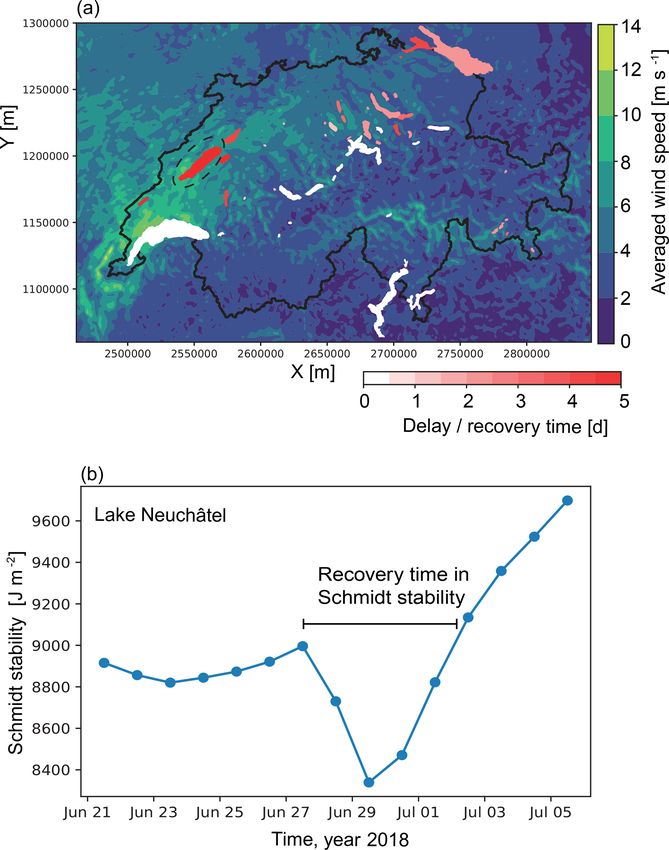
3956                                                                        A. Gaudard et al.: Lake model simstrat.eawag.ch

modellers themselves and often not easily accessible for the        a number of lakes (Gaudard et al., 2017; Perroud et al., 2009;
outside community.                                                  Råman Vinnå et al., 2018; Schwefel et al., 2016; Thiery et
   The performance of lake models is determined by the              al., 2014). Recently, large parts of the code were refactored
physical representativeness of the algorithms and by the            using the object-oriented Fortran 2003 standard. This version
quality of the input data. The latter include (i) lake morphol-     of Simstrat provides a clear, modular code structure. The
ogy, (ii) atmospheric forcing, (iii) hydrological cycle (e.g.,      source code of Simstrat v2.1 is available via GitHub at
inflow, outflow, and/or water level fluctuations), and (iv) light   https://github.com/Eawag-AppliedSystemAnalysis/Simstrat/
absorption. In situ observations, such as temperature pro-          releases/tag/v2.1 (last access: 29 August 2019). A simpler
files, are required for calibration of model parameters. To         build procedure was implemented using a docker container.
support this approach, it is important to promote and facil-        This portable build environment contains all necessary
itate the sharing of existing datasets of observations among        software dependencies for the build process of Simstrat. It
scientists and practitioners. Conversely, scientists and practi-    can therefore be used on both Windows and Linux systems.
tioners should benefit from the model output, which is often        A step-by-step guide is provided on GitHub.
ready to use, high frequency, and up to date. Yet, model out-          In addition to the improvements already described by
put data should not only be seen as a tool for temporal inter-      Schmid and Köster (2016), Simstrat v2.1 includes (i) the pos-
polation of measurements. Models also provide data of hard-         sibility to use gravity-driven inflow and a wind drag coeffi-
to-measure quantities which are helpful for specific analy-         cient varying with wind speed – both described by Gaudard
ses (e.g., the heat content change to assess impact of climate      et al. (2017) – and (ii) an ice and snow module. The ice and
change or the vertical diffusivity to estimate vertical turbu-      snow module employed in the model is based on the work of
lent transport). Models finally support the interpretation of       Leppäranta (2014, 2010) and Saloranta and Andersen (2007),
biogeochemical processes which often depend on the thermal          and is further described in Appendix B.
stratification, mixing, and temperature. In a global context of        A Python script was developed to (i) retrieve the newest
open science, collaboration between the different actors and        forcing data directly from data providers and integrate them
reuse of field and model output data should be fostered. Such       into the existing datasets, (ii) process the input data and
win–win collaboration serves the interests of lake modellers,       prepare the full model and calibration setups, (iii) run the
researchers, field scientists, lake managers, lake users, and       calibration of the model for the chosen model parameters,
the public in general.                                              (iv) provide output results, and (v) update the Simstrat online
   In this work, we present a new automated web-based plat-         data platform to display these results. The script is controlled
form to visualize and distribute the near-real-time (weakly)        by an input file written in JavaScript Object Notation (JSON)
output of the one-dimensional hydrodynamic lake model               format, which specifies the lakes to be modeled together with
Simstrat through an user-friendly web interface. The current        their physical properties (depth, volume, bathymetry, etc.)
version includes 54 Swiss lakes covering a wide range of            and identifies the meteorological and hydrological stations to
characteristics from very small volume such as Inkwilersee          be used for model forcing. The overall workflow is illustrated
(9 × 10⁻³ km3 ) to very large systems such as Lake Geneva           in Fig. 1.
(89 km3 ), over an altitudinal gradient (Lake Maggiore at
from 193 m a.s.l. to Daubensee at 2207 m a.s.l.) and over all       2.2   Input data
trophic states (14 eutrophic lakes, 10 mesotrophic lakes, and
21 oligotrophic lakes; Appendix A). We focus here on de-            Table 1 summarizes the type and sources of the data fed to
scribing the fully automated workflow, which simulates the          Simstrat. For meteorological forcing, homogenized hourly
thermal structure of the lakes and updates the online plat-         air temperature, wind speed and direction, solar radiation,
form weekly (https://simstrat.eawag.ch, last access: 29 Au-         and relative humidity from the Federal Office of Meteo-
gust 2019) with metadata, plots, and downloadable results.          rology and Climatology (MeteoSwiss, Switzerland) weather
This state-of-the-art framework is not restricted to the cur-       stations are used. For each lake, the closest weather stations
rently selected lakes and can be applied to other systems or        are used. Air temperature is corrected for the small alti-
at global scale.                                                    tude difference (see Appendix A) between the lake and the
                                                                    meteorological station, assuming an adiabatic lapse rate of
                                                                    −0.0065 ◦ C m−1 . This correction is a source of error in high-
2     Methods                                                       altitude lakes like Daubensee for which dedicated meteoro-
                                                                    logical station would be needed. The cloud cover needed for
2.1    Model and workflow                                           downwelling longwave radiations are estimated by compar-
                                                                    ing observed and theoretical solar radiation (Appendix C).
We use the 1-D lake model Simstrat v2.1 to model 54 Swiss           For hydrological forcing, homogenized hourly data from the
lakes or reservoirs (see Appendix A for details of modeled          stations operated by the Federal Office for the Environment
lakes) in an automated way. Simstrat was first introduced by        (FOEN) are used. For each lake, the data from the available
Goudsmit et al. (2002) and has been successfully applied to         stations at the inflows are aggregated to feed the model with

Geosci. Model Dev., 12, 3955–3974, 2019                                                www.geosci-model-dev.net/12/3955/2019/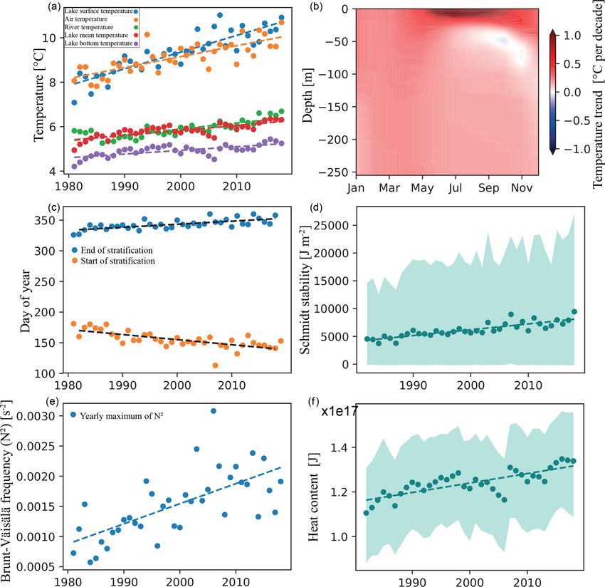
A. Gaudard et al.: Lake model simstrat.eawag.ch                                                                               3957

Figure 1. General workflow diagram. Model input (a) is retrieved and processed by the Python script “Simstrat.py”, which runs
the model (Simstrat v2.1) and/or model calibration (using PEST v15.0) (b) and produces output (c). This output is then uploaded
to a web interface (https://simstrat.eawag.ch, last access: 29 August 2019) for general use. All scripts and programs are available
on https://github.com/Eawag-AppliedSystemAnalysis/Simstrat/releases/tag/v2.1 (last access: 29 August 2019) and https://github.com/
Eawag-AppliedSystemAnalysis/Simstrat-WorkflowModellingSwissLakes (last access: 29 August 2019). Simstrat is the one-dimensional
hydrodynamic model; CTD is a conductivity–temperature–depth profiler; PEST is the model-independent parameter estimation and uncer-
tainty analysis software; FOEN is the Swiss Federal Office of Environment; MeteoSwiss is the Swiss Federal Office of Meteorology and
Climatology; Swisstopo is the Swiss Federal Office of Topography.

Table 1. Input data sources used for the model.

           Data                      Source                             Model input
           Lake bathymetry           Swisstopo                          Bathymetry profile
                                     (https://www.swisstopo.admin.ch,
                                     last access: 29 August 2019)
           Meteorological forcing    MeteoSwiss                         Air temperature, solar radiation, humidity, wind,
                                     (http://meteoswiss.admin.ch,       cloud cover, precipitation
                                     last access: 29 August 2019)
           Hydrological forcing      FOEN                               Inflow discharge, inflow temperature
                                     (http://hydrodaten.admin.ch,
                                     last access: 29 August 2019)
           Secchi depth              Eawag, cantonal monitoring         Light absorption coefficient
           CTD profiles              Eawag, cantonal monitoring         Initial conditions, temperature observations
                                                                        for calibration

www.geosci-model-dev.net/12/3955/2019/                                                 Geosci. Model Dev., 12, 3955–3974, 2019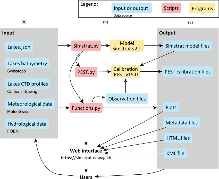
3958                                                                                  A. Gaudard et al.: Lake model simstrat.eawag.ch

Table 2. Model parameters. The geothermal heat flux is based on existing geothermal data for Switzerland: https://www.geocat.ch/
geonetwork/srv/eng/md.viewer\#/full_view/2d8174b2-8c4a-44ea-b470-cb3f216b90d1 (last access: 29 August 2019).

    Parameter           Description and units                                                                     Default value
    lat                 Latitude (◦ )                                                                             Based on lake location
    p_air               Air pressure (mbar)                                                                       Based on lake elevation
    a_seiche∗           Ratio of wind energy going into seiche energy (–)                                         Based on lake size
    q_nn                Fractionation coefficient for seiche energy (–)                                           1.10
    f_wind∗             Scaling factor for wind speed (–)                                                         1.00
    c10                 Scaling factor for the wind drag coefficient (–)                                          1.00
    cd                  Bottom drag coefficient (–)                                                               0.002
    hgeo                Geothermal heat flux (W m−2 )                                                             Based on geothermal map
                                                                                                                  (see table caption)
    p_radin∗            Scaling factor for the incoming longwave radiation (–)                                    1.00
    p_windf             Scaling factor for the fluxes of sensible and latent heat (–)                             1.00
    albsw               Albedo of water for shortwave radiation (–)                                               0.09
    beta_sol            Fraction of shortwave radiation absorbed as heat in the uppermost water layer (–)         0.35
    p_albedo∗           Scaling factor for snow/ice albedo, thereby affecting melting and under ice warming (–)   1.00
    freez_temp          Water freezing temperature (◦ C)                                                          0.01
    snow_temp           Temperature below which precipitation falls as snow (◦ C)                                 2.00

  The asterisk (∗ ) indicates the parameters that were calibrated.

a single inflow. The aggregated discharge is the sum of the                  this approach. Longer data gaps of up to 20 d are replaced
discharge of all inflows, and the aggregated temperature is                  by the long-term average values for the corresponding day of
the weighted average of the inflows for which temperature is                 the year. Only ∼ 1.5 % of the dataset is corrected using this
measured. Inflow data are often missing for small or high-                   approach.
altitude lakes (Appendix A). Missing inflows and more gen-
erally watershed data are a source of error in small alpine                  2.3   Calibration
lakes, yet such error can be compensated during the calibra-
tion process. The light absorption coefficient εabs (m−1 ) is
                                                                             Model parameters are set to default values, and four of
either obtained from Secchi depth zSecchi (m) measurements
                                                                             them are calibrated (see Table 2). The parameters p_radin
(for Inkwilersee, Lake Biel, Lake Brienz, Lake Geneva, Lake
                                                                             and f_wind scale the incoming longwave radiation and the
Neuchâtel, lower Lake Zurich, Oeschinen Lake, upper Lake
                                                                             wind speed, respectively, and can be used to compensate
Constance, and Sihlsee) or set to a constant value based on
                                                                             for systematic differences between the meteorological con-
the lake trophic status. In the first case, the following equa-
                                                                             ditions on the lake and at the closest meteorological station.
tion is applied: εabs = 1.7/zSecchi (Poole and Atkins, 1929;
                                                                             The parameter a_seiche determines the fraction of wind en-
Schwefel et al., 2016). In the second case, εabs is set to
                                                                             ergy that feeds the internal seiches. This parameter is lake-
0.15 m−1 for oligotrophic lakes, 0.25 m−1 for mesotrophic
                                                                             specific, as it depends on the lake’s morphology and its ex-
lakes, and 0.50 m−1 for eutrophic lakes. The values cor-
                                                                             posure to different wind directions. Finally, the parameter
respond to observations of Secchi depths in Swiss lakes
                                                                             p_ albedo scales the albedo of ice and snow applied to in-
(Schwefel et al., 2016) and fall into the decreasing range of
                                                                             coming shortwave radiation, which depends on the ice/snow
transparency from an oligotrophic to eutrophic system (Carl-
                                                                             cover properties. The calibration parameters were selected
son, 1977). For glacier-fed lakes (typical above 2000 m) rich
                                                                             according to their importance for the model (e.g., based on
in sedimentary material, εabs is set to 1.00 m−1 .
                                                                             previous sensitivity analysis), and their number was deliber-
   The timeframe of the model is determined by the avail-
                                                                             ately kept small in order to keep the calibration process sim-
ability of the meteorological data (air temperature, solar
                                                                             ple and focused. Calibration is performed using PEST v15.0
radiation, humidity, wind, precipitation). Initial conditions
                                                                             (see http://pesthomepage.org, last access: 29 August 2019), a
for temperature and salinity are set using conductivity–
                                                                             model-independent parameter estimation software (Doherty,
temperature–depth (CTD) profiles or using the temperature
                                                                             2016). As a reference for calibration, temperature observa-
information from the closest lake. We apply different data
                                                                             tions from CTD profiles are used. Calibration is performed
patching methods to remove data gaps from the forcing de-
                                                                             on a yearly basis, unless significant changes are made ei-
pending on the length of the data gap. For small data gaps
                                                                             ther to the model, the forcing data, or the observational data
with duration not exceeding 1 d, the dataset is linearly in-
                                                                             (e.g., release of a new version of Simstrat or delivery of a
terpolated. In total, < 1 % of the dataset is corrected using
                                                                             large amount of new observational data). For the eight lakes

Geosci. Model Dev., 12, 3955–3974, 2019                                                         www.geosci-model-dev.net/12/3955/2019/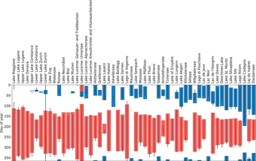
A. Gaudard et al.: Lake model simstrat.eawag.ch                                                                               3959

without observational data, parameters are set to their default     3     Results and discussion
value (see Table 2) with no calibration performed, and the
lack of calibration is indicated on the online platform.            Analysis of model output allows to compare the response
                                                                    of the different systems to specific events or to long-term
2.4   Output/available data on the online platform                  changes. The Simstrat model web interface provides regional
                                                                    long-term high-frequency data updated in near-real time as
The online platform (accessible at https://simstrat.eawag.ch,       output. This represents a novel way to monitor, analyze, and
last access: 29 August 2019) is automatically fed every week        visualize processes in aquatic systems and, most importantly,
with model results, metadata, and plots for all the 54 mod-         grant the entire community direct access to the findings. The
eled lakes (see Fig. 2). It allows for efficient display and open   coupling between Simstrat and PEST provides an effective
sharing of the model results for interested users. While the        way to calibrate model parameters. The uncertainty quan-
framework is here restricted to Swiss lakes, the code could be      tification finally allows an appropriate informed use of the
easily adapted to other lakes outside Switzerland and used at       output data. Yet more advanced methods for both parameter
the global scale. From the model results, we directly obtain        estimation and uncertainty quantification such as Bayesian
time series of several model output variables. Those datasets       inference (Gelman et al., 2013) should be applied to Sim-
include temperature, salinity, Brunt–Väisälä frequency, ver-        strat.
tical diffusivity, and ice thickness. In addition, we use the           Out of the 46 calibrated lakes, the post-calibration root
following known physical and lake-related properties: the ac-       mean square error (RMSE) is < 1 ◦ C for 17 lakes, between
celeration of gravity (g = 9.81 m2 s−1 ), the heat capacity of      1 and 1.5 ◦ C for 15 lakes, between 1.5 and 2 ◦ C for eight
water (cp = 4.18 × 10³ J K−1 kg−1 ), the volume of the lake         lakes and between 2 and 3 ◦ C for six lakes (Fig. 3). There
V (m3 ), the area Az (m2 ), temperature Tz (◦ C), and den-          were too few in situ observations on eight lakes to perform
sity ρzR (kg m−3 ) at depth z (m), and the mean lake depth          a proper calibration and all parameters were thereby set to
z = V1 zAz dz (m) to calculate time series of derived values:       default values. Overall, the performance is comparable to the
                                                                    RMSE range of ∼ 0.7–2.1 ◦ C reported in a recent global 32-
   – mean lake temperature: T = V1 Tz Az dz (◦ C);
                                        R
                                                                    lake modeling study using GLM (Bruce et al., 2018) also in-
                              R
   – heat content: H = cp ρz Tz Az dz (J);                          cluding Lake Geneva, Lake Constance, and Lake Zurich. The
                                                                    correlation coefficient remains always higher than 0.93, sug-
   – Schmidt stability: ST = Ag0 (z − z) ρz Az dz (J m−2 );
                                    R
                                                                    gesting also that the model successfully reproduce the ther-
                                                                    mal structure of the investigated lakes. Overall, the quality of
  – timing of summer stratification: we use a threshold             the results is better for lowland lakes than for high-altitude
    based on the Schmidt stability to determine the begin-          lakes where local meteorological and watershed information
    ning and end of summer stratification. The lake is as-          is often missing.
    sumed to be stratified for ST /zlake ≥ 10 J m−3 . Using             We illustrate the potential of high-frequency lake model
    a different criterion (e.g., temperature difference be-         data with two examples: first by briefly showing the long-
    tween surface and bottom water) results in variations in        term changes caused by climate change in Lake Brienz
    the calculated stratification period; however, the general      (Sect. 3.1), and secondly by investigating the differential re-
    pattern among lakes remains similar;                            sponse of lakes across Switzerland to episodic forcing (short-
                                                                    term extremes; Sect. 3.2).
  – timing of ice cover: we use the existence of ice to deter-
    mine beginning and end of ice covered period.
                                                                    3.1    Long-term evolution of the thermal structure of
   From these results, we create static and interactive plots.             lakes in response to climate trends
The latter are created using the Plotly Python library (see
https://plot.ly/python, last access: 29 August 2019). The plots     Over the period 1981–2015, yearly averaged simulated sur-
can be categorized as follows:                                      face temperatures in Lake Brienz increased with a sig-
                                                                    nificant (p < 0.001) trend of +0.69 ◦ C decade−1 (Fig. 4a).
  – history (e.g., contour plot of the whole temperature time       For the same period, monthly in situ observations indi-
    series, line plot of the whole time series of Schmidt sta-      cate a similar trend of 0.72 ◦ C decade−1 (p ∼ 0.07), while
    bility);                                                        the trend of air temperature at the meteorological sta-
                                                                    tion in Interlaken is lower (+0.50 ◦ C decade−1 , p < 0.01).
  – current situation (e.g., latest temperature profile);
                                                                    Based on physical principles, lake surface temperature is
  – statistics (e.g., average monthly temperature profiles,         expected to increase less than air temperature (Schmid et
    long-term trends).                                              al., 2014); however, Schmid and Köster (2016) also ob-
                                                                    served a higher trend in lake surface temperature than in air
All output and processed data are directly available from the       temperature for lower Lake Zurich and assigned the excess
online platform.                                                    warming to a positive trend in solar radiation. For the pe-

www.geosci-model-dev.net/12/3955/2019/                                                Geosci. Model Dev., 12, 3955–3974, 2019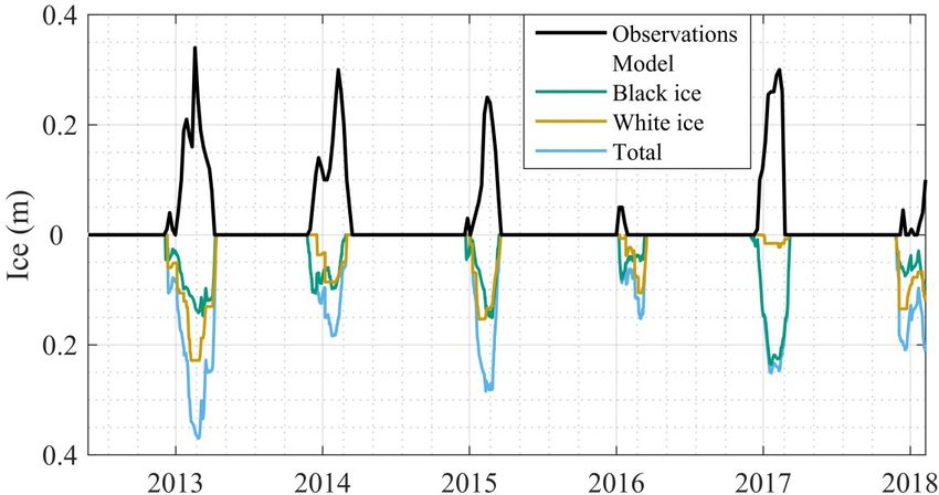
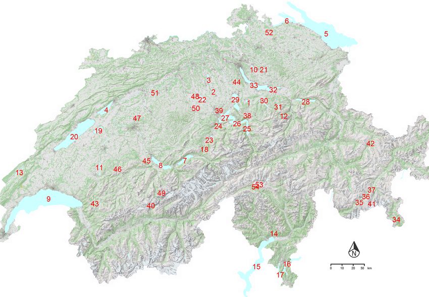
3960                                                                           A. Gaudard et al.: Lake model simstrat.eawag.ch

Figure 2. Illustration of the interactive map displayed on the home page of the online platform: https://simstrat.eawag.ch (last access:
29 August 2019). The locations of the lakes discussed in this paper are also indicated with numbers (see Appendix A). Basemap source:
Federal Office of Topography ©Swisstopo.

riod of 1981–2015, the ascending trend in solar radiation             (p < 0.001). The temperature difference between the inflow
is 5 W m−2 decade−1 , which corresponds to an equilibrium             and the outflow also contributes to the heat budget. While no
temperature increase of about 0.2 ◦ C decade−1 . The warm-            significant change in the yearly total discharge was observed
ing rate at the surface of Lake Brienz is larger than ob-             at the gauging stations of FOEN for the inflows of the Aare
served trends in neighboring lakes with reported increases of         and of the Lütschine rivers for the period 1981–2015, the
+0.46 ◦ C decade−1 for upper Lake Constance (1984–2011;               weighted inflow temperature increased by 0.26 ◦ C decade−1 .
Fink et al., 2014), +0.41 ◦ C decade−1 for lower Lake Zürich          The riverine temperature remains colder than the lake sur-
(1981–2013, Schmid and Köster, 2016; 1955–2013, Living-               face temperature, leading to a yearly average loss of energy
stone, 2003), and +0.55 ◦ C decade−1 for lower Lake Lugano            by throughflow of ∼ −40 W m−2 for 2015. This result is con-
(1972–2013; Lepori and Roberts, 2015). This can be ex-                sistent with the recent observations of Råman Vinnå (2018),
plained by the lower light penetration in Lake Brienz (rang-          suggesting that tributaries significantly affect the thermal re-
ing from ∼ 1 to ∼ 10 m) compared to other lakes, the increase         sponse of lakes with residence time up to 2.7 years (as Lake
in solar radiation being distributed into a shallower layer and       Brienz). The contribution of the river to the heat budget of
thereby warming the lake surface slightly more. This low              Lake Brienz is also ∼ 4 times larger than that previously
light penetration results from upstream hydropower opera-             estimated for upper Lake Constance (Fink et al., 1994), a
tion on the glacier-fed river (Finger et al. 2006).                   lake with a longer residence time. The increasing difference
   The temperature increase was significantly smaller in              over time between the inflow temperature and the outflow
the hypolimnion, with a minimum trend at the lake bot-                temperature (taken as the lake surface temperature) leads
tom of 0.16 ◦ C decade−1 (p < 0.001), leading to a depth-             to a non-negligible cooling contribution from the river of
averaged rate of temperature increase of 0.22 ◦ C decade−1            ∼ 0.14 ◦ C decade−1 (p < 0.05). The temporal change in the

Geosci. Model Dev., 12, 3955–3974, 2019                                                  www.geosci-model-dev.net/12/3955/2019/
A. Gaudard et al.: Lake model simstrat.eawag.ch                                                                                     3961

Figure 3. Performance of the model for the different lakes, as shown by the root mean square error (RMSE) and the correlation coefficient.
Six lakes (with symbol • on the legend) with RMSE > 2 ◦ C are not shown.

discharge and its temperature resulting from climate change            An altitude-dependent decrease of the duration of summer
should therefore be taken into account in studies attempting           stratification is observed, along with a stronger correspond-
to predict the change in lake thermal structure.                       ing increase in the duration of the inverse winter stratifica-
   The vertically heterogeneous warming modeled in Lake                tion from 1200 m a.s.l. This is possibly linked to an altitude
Brienz is consistent with previous observations showing that           dependency of climate-driven warming in Swiss lakes, first
the difference in warming between the surface and the bot-             reported by Livingstone et al. (2005), which may be caused
tom increases the strength and duration of the stratified              by a delay in meltwater runoff (Sadro et al., 2018). Here, this
period (Zhong et al., 2016; Wahl and Peeters, 2014). We                process is not directly resolved but incorporated through the
simulate an earlier onset of the stratification in spring of           calibration procedure spanning all seasons.
−7.5 d decade−1 (p < 0.001) and a later breakdown of the                  In conclusion, the online platform provides all the data to
stratification by +3.7 d decade−1 (p < 0.001) (Fig. 4c). Both          estimate the past warming rate of lakes and evaluate how the
the warming trend and the increase in length of the strat-             different external processes contribute to their heat budgets.
ified period increase the Schmidt stability (Fig. 4d) and              The change in the thermal structure depends mostly on the
heat content (Fig. 4f). Finally, the yearly maximum strat-             change in atmospheric forcing, yet other factors such as the
ification strength (Brunt–Väisälä frequency; Fig. 4e) grad-            changes in discharge and temperature from the tributaries
ual increases over the investigated period with a rate of              and the light absorption into the lake should also be taken
3.3 × 10⁻⁴ s−2 decade−1 . The simulated increase in overall            into account. We specifically show that the warming rate of
stability (Fig. 4d–f) reduces vertical mixing and affects the          the lake surface temperature significantly differs from that
vertical storage of heat with less heat transferred immedi-            of depth-averaged temperature, thereby highlighting the ben-
ately below the thermocline causing a slight decrease in tem-          efit of using either in situ observations resolving the ther-
perature observed in autumn at ∼ 30 m depth (Fig. 4b). This            mal structure over the water column or hydrodynamic model
effect is even more clearly seen in other lakes like Lake              output for assessing climate change impacts on lake thermal
Geneva (https://simstrat.eawag.ch/LakeGeneva, last access:             structure.
29 August 2019) with the surface waters warming strongly
(+1 ◦ C decade−1 in June), resulting in a cooling layer be-            3.2   Event-based evolution of the lake thermal structure
tween 20 and 60 m (−0.2 ◦ C decade−1 ) in late summer. Such
a reduction of vertical exchange is self-strengthening and en-         A major drawback of traditional lake monitoring programs
hances the differential vertical warming.                              in Switzerland is the coarse temporal resolution, with mea-
   Such analyses can be extended to all modeled lakes. An              surements often performed on a monthly basis. This res-
intercomparison of the temporal extent of summer stratifi-             olution only allows to detect long-term trends when mea-
cation and winter ice cover period is illustrated in Fig. 5.           surements are conducted over an extended period typically
                                                                       longer than 30 years. However, traditional monitoring pro-

www.geosci-model-dev.net/12/3955/2019/                                                     Geosci. Model Dev., 12, 3955–3974, 2019
3962 A. Gaudard et al.: Lake model simstrat.eawag.ch
Figure 4. Evolution of several indicators for Lake Brienz over the period 1981–2018; all linear regression have p values
0.001: (a) yearly
mean lake surface temperature (0.69 ◦ C decade−1 ), yearly mean air temperatures (0.49 ◦ C decade−1 ), yearly mean tributary temperatures
(0.26 ◦ C decade−1 ), yearly mean lake temperatures (0.22 ◦ C decade−1 ), and yearly mean bottom temperatures (0.16 ◦ C decade−1 ), with
linear regression, (b) contour plot of the linear temperature trend through depth and month, (c) yearly start (+3.7 d decade−1 ) and end
(−7.5 d decade−1 ) days of summer stratification, with linear regression, (d) yearly mean (line), min, and max (shaded area) Schmidt stability,
with linear regression, (e) yearly maximum Brunt–Väisälä frequency (3.3 × 10⁻⁴ s−2 decade−1 ), with linear regression, (f) yearly mean
(line), min, and max (shaded area) heat content.
grams cannot resolve the impact of short-term events and Here, we demonstrate how high-frequency model output
their consequences for the ecosystem. This is a strength of can be used to study the influence of specific events on the
high-frequency (hourly timescale) lake modeling, which al- thermal dynamics of lakes. As an example, we focus on
lows for simulation and comparison of the effects associated 28 June 2018, when Switzerland experienced a strong but by
with rapid and often severe events such as storms. Based on no means exceptional storm with northeasterly winds mainly
high-frequency observations, Woolway et al. (2018) showed affecting the northwestern part of the country – the mean
the effects of a major storm on Lake Windermere. They ob- wind speed during that day is shown spatially in Fig. 6a.
served a decrease in the strength of the stratification, a deep- The evolution of the stratification strength, illustrated here
ening of the thermocline and the onset of internal waves os- by the Schmidt stability, is given in Fig. 6b for one of the
cillations ultimately upwelling oxygen-depleted cold water most affected lakes, Lake Neuchâtel (https://simstrat.eawag.
into the downstream river. Furthermore, Perga et al. (2018) ch/LakeNeuchatel, last access: 29 August 2019; Fig. 2). This
illustrated how storms could be just as important as gradual lake, with the main axis well aligned to synoptical winds, ex-
long-term trends for changes in light penetration and thermal perienced a ∼ 8 % decrease in the Schmidt stability over this
structure in an alpine lake. half-day event. Yet, the effects were not long-lasting and the
Schmidt stability reverted to its pre-storm value within ∼ 5 d
Geosci. Model Dev., 12, 3955–3974, 2019 www.geosci-model-dev.net/12/3955/2019/A. Gaudard et al.: Lake model simstrat.eawag.ch 3963 Figure 5. Comparison of timing of stratification and ice cover for the considered lakes. The colored areas represent the mean periods of summer stratification (red) and ice cover (blue); the vertical lines represent the last year (here 2017). The transparency for the ice cover indicates the freezing frequency: full transparency means that ice was never modeled, while no transparency means that ice was modeled every winter. Lakes are ordered from left (low elevation) to right (high elevation). The time period of data used is indicated in Appendix A. (Fig. 6b). This also resulted in a total increase of the lake torical forcing reanalysis should be integrated in such web- heat content by ∼ 1.4 × 10¹⁶ J from the start of the storm to based hydrodynamic platforms to assess their roles in modi- the time of recovery. We used the Schmidt stability recovery fying the lake thermal structures and heat storage. duration as a way to assess the short-term effect of the storm on the different modeled lakes. In Fig. 6a, lakes are colored based on the delay in Schmidt stability increase (in days) 4 Conclusion caused by the storm. The impact of the storm was not lim- ited to Lake Neuchâtel but rather showed a regionally vary- The workflow presented in this paper allows openly sharing ing pattern. Particularly small- to medium-sized lakes in the high-frequency, up-to-date and permanently available lake northwestern parts of Switzerland were more affected than model results for multiple users and purposes. We demon- large lakes or lakes located in the southern part of Switzer- strated the benefit of the platform through two simple case land. However, the thermal structure of these lakes quickly studies. First, we showed that the high-frequency modeled reverted to the seasonal early summer warming trend. temperature data allow a complete assessment of the effect of So far, climate-driven warming has been recognized to climate change on the thermal structure of a lake. We specif- cause an overall increase in lake stratification strength and ically show the need to evaluate changes in all atmospheric duration, and a gradual warming of the different layers forcing, in the watershed or throughflow heat energy, and in (Schwefel et al., 2016; Zhong et al., 2016; Wahl and Peeters, light penetration to accurately assess the evolution of the lake 2014). Air temperature trend was the most studied forcing thermal structure. Then, we showed that the high-frequency parameter. Yet, the dynamics of extreme events (such as modeled data can be used to investigate special events such as heat waves, drought spells, storms), including their changes wind storms; there, in situ measurements under current tem- in strength and distribution, has been comparatively over- poral resolution are failing. More generally, these results are looked. Scenario exploration, climate change studies, or his- well suited for the following applications and target groups: www.geosci-model-dev.net/12/3955/2019/ Geosci. Model Dev., 12, 3955–3974, 2019
3964                                                                             A. Gaudard et al.: Lake model simstrat.eawag.ch

                                                                            By promoting a cross exchange of expertise through
                                                                         openly sharing of in situ and model data at high frequency,
                                                                         this open-access data platform is a new path forward for sci-
                                                                         entists and practitioners.

                                                                         Code and data availability. The workflow was developed for
                                                                         Swiss lakes but can be easily extended to other geograph-
                                                                         ical area or at global scale by using other meteorological
                                                                         input data. Simstrat and the Python workflow are avail-
                                                                         able      on     https://github.com/Eawag-AppliedSystemAnalysis/
                                                                         Simstrat/releases/tag/v2.1 (last access: 29 August 2019,
                                                                         https://doi.org/10.5281/zenodo.2600709, Bärenbold et al.,
                                                                         2019) and https://github.com/Eawag-AppliedSystemAnalysis/
                                                                         Simstrat-WorkflowModellingSwissLakes (last access: 29 Au-
                                                                         gust     2019,     https://doi.org/10.5281/zenodo.2607153,   Gau-
                                                                         dard, 2019). Meteorological data are available from Me-
                                                                         teoSwiss      (https://gate.meteoswiss.ch/idaweb/,   last  access:
                                                                         29 August 2019), hydrological data are available from FOEN
                                                                         (https://www.hydrodaten.admin.ch, last access: 29 August 2019),
                                                                         and CTD data were provided by various sources listed here:
                                                                         https://simstrat.eawag.ch/impressum (last access: 29 Au-
                                                                         gust 2019). The calibration software PEST is available on
                                                                         http://www.pesthomepage.org/ (last access: 29 August 2019,
                                                                         Doherty, 2010).

Figure 6. (a) Mean wind field on 28 June 2018 (data source: Me-
teoSwiss, COSMO-1 model, coordinate system CH1903+) and de-
lay in Schmidt stability increase for the modeled lakes: from no
delay (white) to a delay of more than 5 d (red). (b) Schmidt stability
(daily average) in Lake Neuchâtel during the period of the storm.

  – For the public, the platform serves as an informative
    website enabling easy access to broad quantities of re-
    gional scientific results, with the intention of raising in-
    terest about lake ecosystem dynamics.

  – For lake managers, the platform makes relevant infor-
    mation available, such as (i) near-real-time temperature
    and stratification conditions of the lakes and (ii) simple
    statistical analyses such as monthly temperature profiles
    and long-term temperature trends.

  – For researchers, this work can facilitate (i) scenario
    modeling of any of the lakes, as the basic model setup
    is ready to use, (ii) improvement of the lake model
    with addition of previously unresolved processes (e.g.,
    resuspension with changed light properties), (iii) ac-
    cess to variables that were previously not or irregularly
    available (e.g., vertical diffusivity, heat content, strati-
    fication, and heat fluxes), and (iv) specific comparative
    analyses, whereby a given question can be investigated
    simultaneously over many lakes (e.g., the impact of cli-
    mate change or a regional storm).

Geosci. Model Dev., 12, 3955–3974, 2019                                                    www.geosci-model-dev.net/12/3955/2019/
A. Gaudard et al.: Lake model simstrat.eawag.ch 3965
Appendix A: Properties of the modeled lakes
Table A1. This table summarizes the main properties of the 54 lakes we model in this work. The full dataset is available as a JSON file. The
superscript “a” after the lake name indicates that this lake was not calibrated due to the lack of observational data. MeteoSwiss is the (Swiss)
Federal Office of Meteorology and Climatology. FOEN is the (Swiss) Federal Office for the Environment. The superscript “b” indicates lakes
where Secchi disk depths are available. For lakes with clearly defined multiple basins such as Lake Lucerne, Lake Zurich, Lake Constance
and Lake Lugano, each basin is considered as a separated lake connected to the other basins by inflows/outflows.
Max Hydrological Model
Volume Surface depth Retention Elevation Trophic Weather station station IDs time
Lake (km3 ) (km2 ) (m) time (years) (m) state IDs (MeteoSwiss) (FOEN) frame
Lake Aegeri 1 0.36 7.3 83 ∼ 6.8 724 O AEG, SAG, EIN – 2012–2018
689574/
191747
Lake 2 0.174 5.2 66 ∼ 4.2 463 E MOA – 2012–2018
Baldegg
662239/
228077
Lake Hallwil 3 0.285 10.3 48 ∼ 3.9 449 E MOA 2416 2012–2018
658779/
237484
Lake Biel 4 1.12 39.3 74 ∼ 0.16 429 Eb CRM 2085, 2307, 1993–2018
578599/ 2446
214194
Upper Lake 5 47.6 473 251 ∼ 4.3 395 Mb ARH, GUT 2473, 2308, 1981–2018
Constance 2312
749649/
275225
Lower Lake 6 0.8 63 45 ∼ 0.05 395 M STK, HAI, GUT – 1981–2018
Constance
718479/
285390
Lake Brienz 7 5.17 29.8 259 ∼ 2.7 564 Ob INT 2019, 2109 1981–2018
640709/
175275
Lake Thun 8 6.5 48.3 217 ∼ 1.9 558 Ob THU, INT 2457, 2469, 1981–2018
619899/ 2488
172630
Lake Geneva 9 89 580 309 ∼ 11 372 Mb PUY 2009, 2432, 1981–2018
533600/ 2433, 2486,
144624 2493
Greifensee 10 0.15 8.5 32 ∼ 1.1 435 E SMA – 1981–2018
693699/
245032
Lake of 11 0.22 9.6 75 ∼ 0.4 677 NA MAS, GRA 2160, 2412 2011–2018
Gruyère
573990/
168654
www.geosci-model-dev.net/12/3955/2019/ Geosci. Model Dev., 12, 3955–3974, 20193966 A. Gaudard et al.: Lake model simstrat.eawag.ch
Table A1. Continued.
Max Hydrological Model
Volume Surface depth Retention Elevation Trophic Weather station station IDs time
Lake (km3 ) (km2 ) (m) time (years) (m) state IDs (MeteoSwiss) (FOEN) frame
Klöntalersee 12 0.056 3.3 45 ∼ 0.5 848 O GLA – 1981–2018
716984/
209627
Lac de Joux 13 0.145 8.77 32 0.85 1004 M CHB, BIE – 2009–2018
511590/
165965
Lago di 14 0.1 1.68 204 – 470 O OTL 2605 1981–2018
Vogornoa
709279/
118833
Lake 15 37 212 372 ∼4 193 O OTL 2068, 2368 1981–2018
Maggiore
694300/
92576
Upper Lake 16 4.69 27.5 288 ∼ 12.3 271 E LUG 2321 1981–2018
Lugano
721139/
95471
Lower Lake 17 1.14 20.3 95 ∼ 1.4 271 M LUG 2629, 2461 1981–2018
Lugano
714239/
86391
Lake 18 0.065 2 68 ∼ 0.6 688 NA GIH – 2010–2018
Lungern
655099/
183325
Lake Murten 19 0.55 22.8 45 ∼ 1.2 429 Mb NEU 2034 1981–2018
572700/
198094
Lake 20 13.8 218 152 ∼ 8.2 429 Mb NEU 2378, 2369, 1981–2018
Neuchâtel 2480, 2458,
554800/ 2447
194974
Lake 21 0.059 3.3 36 ∼ 2.1 537 M SMA – 1981–2018
Pfäffikon
701604/
245377
Lake 22 0.66 14.5 87 ∼ 16.9 504 M EGO 2608 2010–2018
Sempach
654629/
221355
Lake Sarnen 23 0.239 7.5 51 ∼ 0.8 469 O GIH – 2010–2018
658349/
190767
Geosci. Model Dev., 12, 3955–3974, 2019 www.geosci-model-dev.net/12/3955/2019/A. Gaudard et al.: Lake model simstrat.eawag.ch 3967
Table A1. Continued.
Max Hydrological Model
Volume Surface depth Retention Elevation Trophic Weather station station IDs time
Lake (km3 ) (km2 ) (m) time (years) (m) state IDs (MeteoSwiss) (FOEN) frame
Lake 24 0.1 4.5 35 ∼ 0.3 434 O LUZ 2102, 2436 1981–2018
Lucerne:
Alpnach-
ersee
667144/
202267
Lake 25 3.16 22 200 ∼ 2.0 434 O ALT 2056, 2276 1981–2018
Lucerne:
Urnersee
688649/
200895
Lake 26 4.41 30 214 ∼ 1.6 434 O GES, ALT 2084, 2481 1981–2018
Lucerne:
Gersauer
Becken and
Treibbecken
681659/
203585
Lake 27 4.35 59 151 ∼ 0.7 434 O LUZ – 1981–2018
Lucerne:
Kreuztrichter
and Vitz-
nauerbecken
672049/
208875
Walensee 28 2.5 24.2 151 ∼ 1.4 419 O QUI, LAC, GLA 2372, 2426 1981–2018
735739/
202690
Lake Zug 29 3.2 38.3 197 ∼ 14.7 417 E CHZ, WAE 2477 1981–2018
680049/
216865
Sihlsee 30 0.096 11.3 22 ∼ 0.4 889 O EIN 2300, 2635 2012–2018
701504/
222387
Wägitalerseea 31 0.15 4.18 65 ∼ 1.6 900 O LAC, EIN – 2012–2018
701504/
222387
Upper Lake 32 0.47 20.3 48 ∼ 0.69 406 M WAE 2104 1981–2018
Zurich
707159/
229595
Lower Lake 33 3.36 68.2 136 ∼ 1.4 406 Mb LAC, SCM, WAE – 1981–2018
Zurich
687209/
237715
Lago di 34 0.12 1.98 85 ∼ 0.5 962 O ROB 2078 1981–2018
Poschiavo
804706/
128871
www.geosci-model-dev.net/12/3955/2019/ Geosci. Model Dev., 12, 3955–3974, 20193968 A. Gaudard et al.: Lake model simstrat.eawag.ch
Table A1. Continued.
Max Hydrological Model
Volume Surface depth Retention Elevation Trophic Weather station station IDs time
Lake (km3 ) (km2 ) (m) time (years) (m) state IDs (MeteoSwiss) (FOEN) frame
Lake Sils 35 0.137 4.1 71 ∼ 2.2 1797 O SIA – 2014–2018
776533/
143922
Lake Silva- 36 0.14 2.7 77 ∼ 0.7 1791 O SIA – 2014–2018
plana
780801/
146926
Lake 37 0.02 0.78 44 ∼ 0.1 1768 O SAM 2105 1981–2018
St. Moritz
784870/
152099
Lake Lauerz 38 0.0234 3.07 14 ∼ 0.3 447 M GES, LUZ – 1981–2018
688864/
209546
Rotsee 39 0.00381 0.48 16 ∼ 0.4 419 E LUZ – 1981–2018
666491/
213558
Daubenseea 40 0.64 50 NA 2207 O BLA – 2013–2018
613862/
140026
Lej da 41 0.43 50 NA 2160 O SIA – 2014–2018
Vadreta
785308/
141515
Lake Davosa 42 0.0156 0.59 54 NA 1558 O DAV – 1981–2018
784261/
188317
Lac de 43 0.0532 1.6 105 NA 1250 O CHD – 2012–2018
l’Hongrina
569975/
141537
Türlersee 44 0.00649 0.497 22 ∼2 643 E WAE – 1981–2018
680514/
235858
Amsoldinger- 45 0.00255 0.382 14 NA 641 Eb THU – 2012–2018
see
610534/
174906
Lac Noira 46 0.00252 0.47 10 NA 1045 M PLF – 1989–2018
587970/
168280
Moossee 47 0.00339 0.31 21 NA 521 E BER – 1981–2018
603165/
207928
Mauensee 48 0.55 9 NA 504 E EGO – 2010–2018
648258/
224587
Geosci. Model Dev., 12, 3955–3974, 2019 www.geosci-model-dev.net/12/3955/2019/A. Gaudard et al.: Lake model simstrat.eawag.ch 3969
Table A1. Continued.
Max Hydrological Model
Volume Surface depth Retention Elevation Trophic Weather station station IDs time
Lake (km3 ) (km2 ) (m) time (years) (m) state IDs (MeteoSwiss) (FOEN) frame
Oeschinen 49 0.0402 1.11 56 ∼ 1.6 1578 O ABO – 1983–2018
Lake
622116/
149701
Soppensee 50 0.00286 0.25 27 ∼ 3.1 596 E EGO – 2010–2018
648765/
215720
Inkwilersee 51 0.00094 0.102 6 ∼ 0.1 461 Eb KOP – 2011–2018
617009/
227527
Hüttwilersee 52 0.34 28 NA 434 E HAI – 2010–2018
705538/
274275
Lake 53 0.00242 0.26 21 ∼ 1.5 1921 E PIO – 1981–2018
Cadagno
697683/
156223
Lago Ritoma 54 0.048 1.49 69 NA 1850 O PIO – 1981–2018
695933/
155169
www.geosci-model-dev.net/12/3955/2019/ Geosci. Model Dev., 12, 3955–3974, 20193970 A. Gaudard et al.: Lake model simstrat.eawag.ch
Table A2. Meteorological stations. – melting of snow, white and black ice due to both the
direct heat flux through the atmospheric interface and
Meteorological Altitude Coordinates the absorption of shortwave irradiance.
station Abbreviation (m a.s.l) (CH)
Three layers are used to represent black ice, white ice, and
Oberägeri AEG 724 688728/220956
Sattel SAG 790 690999/215145 snow. An instant supply of water through cracks in the black
Einsiedeln EIN 911 699983/221068 ice is assumed to occur in order to form white ice. The water
Mosen MOA 453 660128/232851 stored in ice and snow is neither withdrawn during ice forma-
Cressier CRM 430 571163/210797 tion nor added during melting to the water balance. Further-
Altenrhein ARH 398 760382/261387
Güttingen GUT 440 738422/273963
more, the effect of liquid water pools on top of or between
Steckborn STK 397 715871/280916 the layers is neglected.
Salen-Reutenen HAI 719 719099/279047
Interlaken INT 577 633023/169092 B1 Below the freezing point (ice formation)
Thun THU 570 611201/177640
Pully PUY 456 540819/151510 The ice module is activated as the water temperature in the
Zürich/ SMA 556 685117/248066 topmost grid cell Tw (◦ C) drops below the freezing temper-
Fluntern
Marsens MAS 715 571758/167317
ature Tf (◦ C). Tf can be set to zero for a vertical grid size
Fribourg/Posieux GRA 651 575184/180076 ≤ 0.5 m; the user can adapt (raise) this value to fit coarser
Les Charbonnières CHB 1045 513821/169387 grids. If temperature is below the freezing point, the energy
Bière BIE 684 515888/153210 incorporated into the change of state Ef is calculated as
Locarno/Monti OTL 367 704172/114342
Lugano LUG 273 717874/95884 Ef = ρw cpw z1 (Tf − Tw ). (B1)
Giswil GIH 471 657322/188976
Neuchâtel NEU 485 563087/205560 Here, ρw (1000 kg m−3 ) is the density of freshwater, cpw the
Egolzwil EGO 522 642913/225541
Luzern LUZ 454 665544/209850
heat capacity of water (4182 J kg−1 ◦ C−1 ), and z1 the height
Altdorf ALT 438 690180/193564 of the topmost grid cell. Ef and the latent heat of freezing
Gersau GES 521 682510/205572 lh (3.34 × 10⁵ J kg−1 ) as well as the density of black ice ρib
Quinten QUI 419 734848/221278 (916.2 kg m−3 ) are used for calculating the initial height of
Laschen/ LAC 468 707637/226334 black ice hib (m) in Eq. (B2); thereafter, Tw is set equal to Tf :
Galgenen
Glarus GLA 517 723756/210568
hib = Ef / (lh ρib ) . (B2)
Cham CHZ 443 677758/226878
Wädenswil WAE 485 693847/230744
If ice cover is present and if the atmospheric temperature
Schmerikon SCM 408 713725/231533
Plaffeien PLF 1042 586825/177407 Ta (◦ C) is smaller than or equal to Tf , the growth of black
Segl-Maria SIA 1804 778575/144977 ice dhib /dt continues as described in Saloranta and Ander-
Blatten, BLA 1538 629564/141084 sen (2007).
Lötschental
Adelboden ABO 1322 609350/149001 dhib p
Piotta PIO 990 695880/152265 = 2ki / (ρib × lh ) × (Tf − Ti ) (B3)
dt
Here, ki (2.22 W K−1 m−1 ) is the thermal conductivity of ice
at 0 ◦ C and Ti (◦ C) the ice temperature calculated as
Appendix B: Ice module P T f + Ta
Ti = (B4)
1+P
The ice and snow module employed is based on the work of
Leppäranta (2014, 2010) and Saloranta and Andersen (2007), ki hs 1
P = max , . (B5)
and includes the following physical processes: ks hib 10hib
– air-temperature-dependent formation and growth of There, ks (0.2 W K−1 m−1 ) is the thermal conductivity of
black ice, including the insulating effect of a snow snow and hs (m) the height of the snow layer. When Ta
cover; is smaller than the snow temperature (default set to 2 ◦ C),
water-equivalent precipitation pr (m h−1 ) is turned into fresh
– snow layer build-up, including the compression effect snow hs_new (m) as
due to the weight of fresh snow;
ρw
hs_new = pr , (B6)
– buoyancy-driven formation of white ice; ρs0
– shortwave irradiance reflection and penetration into the where ρs0 (250 kg m−3 ) is the initial snow density. The exist-
underlying water column; and ing snow cover hs (m) undergoes compression (first terms of
Geosci. Model Dev., 12, 3955–3974, 2019 www.geosci-model-dev.net/12/3955/2019/A. Gaudard et al.: Lake model simstrat.eawag.ch 3971
Eqs. B7 and B8) by the new layer as described in Yen (1981); irradiance through each layer depends on each layer’s thick-
thereafter, the new and existing layers are combined in both ness hx as well as on the layer-specific bulk attenuation co-
height and density (second terms of Eqs. B7 and B8). efficient λx (m−1 ; default λs = 24, λiw = 3, and λib = 2; Lep-
päranta, 2014).
dhs ρs
= −hs 1 − + hs_new (B7)
dt [ρs + dρs ] Hs_s = Is Ap (1 − Ax ) 1 − e(−λs hs ) (B14)
dρs ρs hs + ρs0 hs_new
= ρs C1 ws e−C2 ρs − ρs −
(B8) Hs_iw = Is Ap (1 − Ax ) e(−λs hs ) − e(−λs hs −λiw hiw ) (B15)
dt hs + hs_new
Here, ρs (kg m−3 ) is the snow layer density kept within ρs0 < Hs_ib = Is Ap (1 − Ax ) e(−λs hs −λiw hiw )
ρs < ρsm with the maximum snow density set to 450 kg m−3 ,
C1 (5.8 m−1 h−1 ) and C2 (0.021 m3 kg−1 ) are snow compres- −e(−λs hs −λiw hiw −λib hib ) (B16)
sion constants, and ws (m) is the total weight above the layer
under compression expressed in water-equivalent height. Hs_w = Is Ap (1 − Ax ) 1 − e(−λs hs −λiw hiw −λib hib ) . (B17)
If the snow mass ms (kg m−2 ) becomes heavier than the
There, Hs_w is the radiation penetrating through the ice
upward acting buoyancy force Bi (kg m−2 ), white ice with
cover to the water below and Is (W m−2 ) the incoming short-
height hiw (m) and density ρiw (875 kg m−3 ; Saloranta, 2000)
wave irradiance. We introduce the albedo parameter Ap ,
is formed between the snow and the black ice layers to
which tunes shortwave irradiance in order to match observed
achieve equilibrium between Bi and ms .
water temperatures, thus adjusting the melting and indirectly
Bi = hib (ρw − ρib ) + hiw (ρw − ρiw ) (B9) the duration of the ice cover. Furthermore, depending on
dhiw ms − B i which layer is in contact with the atmosphere, we use a layer-
= (B10) dependent constant albedo Ax (default As = 0.7, Aiw = 0.4,
dt ρs
and Aib = 0.3; Leppäranta, 2014).
In this model, we assume continuous supply of water
through cracks in the black ice to form white ice. The forma- As , hs > 0
tion of white ice takes place instantaneously each time step Ax Aiw , hs = 0 & hiw > 0 (B18)
and we do not consider the influence of pools under the snow
Aib , hs + hiw = 0
for melting or shortwave irradiance penetration.
Calculating Ha requires the longwave emission param-
B2 Above the freezing point (melting) eters ka = 0.68, kb = 0.036 (mbar−1 ), and kc = 0.18 (Lep-
päranta, 2010), atmospheric water vapor pressure ea (mbar),
If ice cover is present and if Ta > Tf , melting starts. Each
cloud cover C, and the Stefan–Boltzmann constant σ (5.67 ×
layer melts from above through the atmospheric interface and
10−8 W m−2 K−4 ). For Eqs. (B19) and (B20), the temper-
by penetrating shortwave radiation:
ature Tx is given in Kelvin. Hw_x is layer dependent for
dhx_upper Hx_y the emissivity Ex with Eiw = Eib = 0.97 and Es (ρs ) from
=− , (B11)
dt (lh + le ) ρx 0.8 at ρs = 250 kg m−3 to Es = 0.9 for ρs = 450 kg m−3 .
Calculating Hk and Hv requires the atmospheric density
where Hx_y (W m−2 ) is the layer-dependent heat flux (in ρa = 1.2 kg m−3 , the heat capacity of air cpa = 1005 J kg−1
the following, subscript x represents the subscript letters “s”, K−1 , the wind speed at 10 m height w10 , the convective
“iw”, or “ib”). The model supports melting through both sub- (bc ) and latent (bl ) bulk exchange coefficients both set to
limation (solid to gas) and non-sublimation (solid to liquid) 0.0015 (Leppäranta, 2010; Gill, 1982), as well as the spe-
with the inclusion/exclusion of the latent heat of evapora- cific humidity of both measured qa (mbar) and at saturation
tion le (J kg−1 ). Non-sublimation melting is default with le q0 . There, qa = 0.622ea /pa , where pa is the air pressure and
set to zero; for sublimation melting, the user can set le to q0 = 0.622 × 6.11/pa at Ta = 0 ◦ C (Leppäranta, 2014).
2265 kJ kg−1 . For the uppermost layer (y = top; Eq. B12),
the heat flux includes layer-dependent uptake of shortwave √ h i
radiation Hs_x , longwave absorption Ha , or layer-dependent Ha = ka + kb ea 1 + kc C 2 σ Ta4 (B19)
emission Hw_x , as well as sensible Hk and latent Hv heat. If
the layer is not in direct contact with the atmosphere, only Hw_x = Ex σ Tf4 (B20)
Hs is used for melting from above (y = under; Eq. B13). Hk = ρa cpa bc (Ta − Tf ) w10 (B21)
Hv = ρa lh bl (qa − q0 ) w10 (B22)
Hx_top = Hs_x + Ha + Hw_x + Hk + Hv (B12)
Hx_under = Hs_x (B13) As Hs_w warms the water under the ice, melting takes
place from underneath with the energy Hbottom (W m−2 ):
Here, we follow Leppäranta (2014, 2010) for determining the
heat flux terms in Eq. (B12). The transmittance of shortwave Hbottom = (Tw − Tf ) cpw ρw z1 . (B23)
www.geosci-model-dev.net/12/3955/2019/ Geosci. Model Dev., 12, 3955–3974, 20193972 A. Gaudard et al.: Lake model simstrat.eawag.ch
After obtaining Hbottom , the temperature of the first cell is
set to Tf and the decrease of ice cover from below becomes
dhx_lower Hbottom
=− . (B24)
dt lm ρx
Equation (B24) is only applied to hib and hiw . In principle,
hs melts completely from above using Eq. (B11) before hib
and hiw reach zero; however, if no ice is present, hs is set to
zero. By combining Eqs. (B11) and (B24), the total melting
of each ice layer is calculated as
dhx dhx_lower dhx_upper
= + . (B25)
dt dt dt Figure B1. Ice model performance in Sihlsee (2012 to 2018) show-
ing modeled white ice (orange), black ice (green), and total ice
When hx < 0 due to melting, the surplus energy is used for cover (white and black ice combined, in blue) against measurements
melting neighboring layers according to the following proce- (black).
dure: if the melting is initiated from above, the surplus energy
is used to melt the layer directly underneath; if the melting is
caused by the water below, the layer directly above receives ϕ is the latitude in radians and H is the hour of the day,
the surplus melting energy; if hibA. Gaudard et al.: Lake model simstrat.eawag.ch 3973
Author contributions. The new version of Simstrat was developed Fink, G., Schmid, M., Wahl, B., Wolf, T., and Wüest, A.: Heat flux
by FB, AG, and LRV. The workflow was developed by AG. The ice modifications related to climate-induced warming of large Euro-
model was developed by LVR. The concept of the workflow was de- pean lakes, Water Resour. Res., 50, 2072–2085, 2014.
fined by DB. All authors contributed to the validation of the model Gaudard, A.: Simstrat-WorkflowModellingSwissLakes (Version
and interpretation of the results. AG and DB wrote the manuscript v1.0), Zenodo, https://doi.org/10.5281/zenodo.2607153, 2019.
with contributions from FB, LVR, and MS. Gaudard, A., Schwefel, R., Vinnå, L. R., Schmid, M., Wüest, A.,
and Bouffard, D.: Optimizing the parameterization of deep mix-
ing and internal seiches in one-dimensional hydrodynamic mod-
Competing interests. The authors declare that they have no conflict els: a case study with Simstrat v1.3, Geosci. Model Dev., 10,
of interest. 3411–3423, https://doi.org/10.5194/gmd-10-3411-2017, 2017.
Gelman, A., Carlin, J., Stern, H., and Rubin, D.: Bayesian Data
Analysis, 3rd edn., Chapman and Hall/CRC, New York, 2013.
Acknowledgements. We thank Davide Vanzo for helping with the Gill, A. E.: Atmosphere-Ocean Dynamics, Academic Press, San
docker and the scripts, and Michael Pantic for helping restructuring Diego, California, USA, ISBN 0-12-283520-4, 1982.
version 2.1 of Simstrat. We finally thank Marie-Elodie Perga for her Goudsmit, G.-H., Burchard, H., Peeters, F., and Wüest, A.: Ap-
comments on a preliminary version of the paper. The full list of ac- plication of k − turbulence models to enclosed basins: The
knowledgements regarding in situ observations can be found here: role of internal seiches, J. Geophys. Res.-Oceans, 107, 3230,
https://simstrat.eawag.ch/impressum (last access: 29 August 2019). https://doi.org/10.1029/2001JC000954, 2002.
Gray, D. K., Hampton, S. E., O’Reilly, C. M., Sharma, S., and
Cohen, R. S.: How do data collection and processing meth-
ods impact the accuracy of long-term trend estimation in lake
Review statement. This paper was edited by Min-Hui Lo and re-
surface-water temperatures?, Limnol. Oceanogr.-Meth., 16, 504–
viewed by three anonymous referees.
515, https://doi.org/10.1002/lom3.10262, 2018.
Hamilton, D. P., Carey, C. C., Arvola, L., Arzberger, P., Brewer,
C., Cole, J. J., Gaiser, E., Hanson, P. C., Ibelings, B. W., Jen-
References nings, E., Kratz, T. K., Lin, F.-P., McBride, C. G., Marques,
M. D. de, Muraoka, K., Nishri, A., Qin, B., Read, J. S., Rose,
Antenucci, J. and Imerito, A.: The CWR dynamic reservoir simula- K. C., Ryder, E., Weathers, K. C., Zhu, G., Trolle, D., and
tion model DYRESM, Science Manual, The University of West- Brookes, J. D.: A Global Lake Ecological Observatory Network
ern Australia, Perth, Australia, 2000. (GLEON) for synthesising high-frequency sensor data for valida-
Bärenbold, F., Gaudard, A., and Raman Vinna, tion of deterministic ecological models, Inland Waters, 5, 49–56,
L.: Simstrat v2.1 (Version v2.1), Zenodo, https://doi.org/10.5268/IW-5.1.566, 2015.
https://doi.org/10.5281/zenodo.2600709, 2019. Hipsey, M. R., Bruce, L. C., and Hamilton, D. P.: GLM – General
Bruce, L. C., Frassl, M. A., Arhonditsis, G. B., Gal, G., Hamil- Lake Model. Model overview and user information, Technical
ton, D. P., Hanson, P. C., Hetherington, A. L., Melack, J. M., Manual, The University of Western Australia, Perth, Australia,
Read, J. S., Rinke, K., Rigosi, A., Trolle, D., Winslow, L., available at: http://swan.science.uwa.edu.au/downloads/AED_
Adrian, R., Ayala, A. I., Bocaniov, S. A., Boehrer, B., Boon, C., GLM_v2_0b0_20141025.pdf (last access: 29 August 2019),
Brookes, J. D., Bueche, T., Busch, B. D., Copetti, D., Cortés, 2014.
A., de Eyto, E., Elliott, J. A., Gallina, N., Gilboa, Y., Guyen- Jennings, E., Eyto, E., Laas, A., Pierson, D., Mircheva, G., Nau-
non, N., Huang, L., Kerimoglu, O., Lenters, J. D., MacIn- moski, A., Clarke, A., Healy, M., Šumberová, K., and Langen-
tyre, S., Makler-Pick, V., McBride, C. G., Moreira, S., Özkun- haun, D.: The NETLAKE Metadatabae – A Tool to Support Au-
dakci, D., Pilotti, M., Rueda, F. J., Rusak, J. A., Samal, N. tomatic Monitoring on Lakes in Europe and Beyond, Limnol.
R., Schmid, M., Shatwell, T., Snorthheim, C., Soulignac, F., Oceanogr., 26, 95–100, https://doi.org/10.1002/lob.10210, 2017.
Valerio, G., van der Linden, L., Vetter, M., Vinçon-Leite, B., Kiefer, I., Odermatt, D., Anneville, O., Wüest, A., and Bouf-
Wang, J., Weber, M., Wickramaratne, C., Woolway, R. I., Yao, fard, D.: Application of remote sensing for the optimization
H., and Hipsey, M. R.: A multi-lake comparative analysis of of in-situ sampling for monitoring of phytoplankton abun-
the General Lake Model (GLM): Stress-testing across a global dance in a large lake, Sci. Total Environ., 527–528, 493–506,
observatory network, Environ. Model. Softw., 102, 274–291, https://doi.org/10.1016/j.scitotenv.2015.05.011, 2015.
https://doi.org/10.1016/j.envsoft.2017.11.016, 2018. Lepori, F., and Roberts, J. J.: Past and future warming of a deep
Burchard, H., Bolding, K., and Villarreal, M. R.: GOTM, a general European lake (Lake Lugano): What are the climatic drivers?, J.
ocean turbulence model: theory, implementation and test cases, Great Lakes Res., 41, 973–981, 2015.
Space Applications Institute, 1999. Leppäranta, M.: Modelling the Formation and Decay of Lake Ice,
Carlson, R. E.: A trophic state index for lakes, Limnol. Oceanogr., in: The Impact of Climate Change on European Lakes, edited by:
22, 361–369, 1977. George, G., Springer Netherlands, Dordrecht, 63–83, 2010.
Doherty, J.: PEST, Model-independent parameter estimation – Leppäranta, M.: Freezing of lakes and the evolution of their ice
User manual (5th edn., with slight additions): Brisbane, Aus- cover, Springer, New York, 2014.
tralia, Watermark Numerical Computing, available at: http:// Livingstone, D. M.: Impact of secular climate change on the ther-
www.pesthomepage.org/ (last access: 29 August 2019), 2010. mal structure of a large temperate central European lake, Clim.
Doherty, J.: PEST: Model-Independent Parameter Estimation, 6th Change, 57, 205–225, 2003.
edn., Watermark Numerical Computing, Australia, 2016.
www.geosci-model-dev.net/12/3955/2019/ Geosci. Model Dev., 12, 3955–3974, 2019You can also read