The presence and stability of DNA mini-hairpins - Hana Bu ˇšková MASTER THESIS
←
→
Page content transcription
If your browser does not render page correctly, please read the page content below
MASTER THESIS

                    Hana Buš̌ková

The presence and stability of DNA
          mini-hairpins

            Department of Low-Temperature Physics

 Supervisor of the master thesis: Mgr. Václav Římal, Ph.D.
             Study programme: Biophysics and Chemical Physics
                 Study branch: Biophysics

                          Prague 2021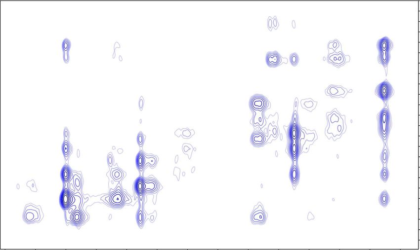
I declare that I carried out this master thesis independently, and only with the
cited sources, literature and other professional sources. It has not been used to
obtain another or the same degree.
I understand that my work relates to the rights and obligations under the Act
No. 121/2000 Sb., the Copyright Act, as amended, in particular the fact that the
Charles University has the right to conclude a license agreement on the use of this
work as a school work pursuant to Section 60 subsection 1 of the Copyright Act.

In Prague, 22nd of July, 2021                .....................................
                                                       Author’s signature

                                         i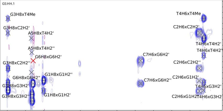
I would like to express my gratitude to my supervisor, Mgr. Václav Římal, PhD.,
for his enormous patience, and to my consultant doc. RNDr. Jan Lang, Ph.D.
for providing valuable feedback. I would also like to thank my family, for giving
me a helping hand, head, and ear, even when I didn’t know I needed it.

                                       ii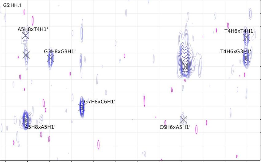
Title: The presence and stability of DNA mini-hairpins

Author: Hana Buš̌ková

Department: Department of Low-Temperature Physics

Supervisor: Mgr. Václav Římal, Ph.D., Department of Low-Temperature Physics

Abstract: The secondary structure of DNA is variable and depends on the se-
quence of nucleotides in a strand. While DNA can form duplexes, formations of
three, four, or even a single strand have been observed in vivo and in vitro as well.
In this thesis, we study the effect of small changes of oligonucleotide sequences on
the stability of hairpins formed by DNA heptamers by 1 H nuclear magnetic reso-
nance (NMR) spectroscopy. Suitable DNA sequences were selected based on sym-
metry rules and stability prediction by nearest neighbor model. Two-dimensional
1
  H -1 H NOESY spectra were used to assign the 1 H resonances of aromatic hydro-
gens. Variable-temperature 1D spectra served for obtaining melting curves, from
which the thermodynamic properties of the hairpins were determined. The pres-
ence of hairpins in the solutions was confirmed by the character of the NOESY
spectra, independence of melting temperature on oligonucleotide concentration,
and comparison of competing melting-curve models of duplex and hairpin. Our
results point out the importance of the order of the stem base pairs and contribute
to the description of the extraordinary stability of DNA mini-hairpins.

Keywords: NMR spectroscopy, DNA, hairpins

                                         iii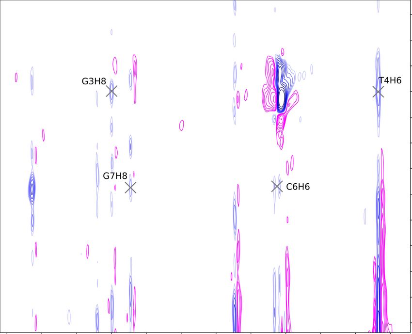
Contents
Introduction                                                                                                               3

1 Deoxyribonucleic acid                                                                                                    4
  1.1 Conformations of nucleotides    .   .   .   .   .   .   .   .   .   .   .   .   .   .   .   .   .   .   .   .   .    4
  1.2 Secondary structure . . . . .   .   .   .   .   .   .   .   .   .   .   .   .   .   .   .   .   .   .   .   .   .    7
  1.3 DNA duplex . . . . . . . . .    .   .   .   .   .   .   .   .   .   .   .   .   .   .   .   .   .   .   .   .   .    7
  1.4 Hairpin formation . . . . . .   .   .   .   .   .   .   .   .   .   .   .   .   .   .   .   .   .   .   .   .   .    8

2 Thermodynamics of processes in an aqueous solution                                                                      9
  2.1 General reaction in an aqueous solution . . . . . . . . .                                   . . . . . .             9
  2.2 Two-state system with hairpin
      and single strand . . . . . . . . . . . . . . . . . . . . .                                 . . . . . .              9
  2.3 Two-state system with duplex
      and single strand . . . . . . . . . . . . . . . . . . . . .                                 . . . . . .             10
  2.4 Three-state system with duplex, hairpin,
      and single strand . . . . . . . . . . . . . . . . . . . . .                                 . . . . . .             11
  2.5 Nearest-neighbor model . . . . . . . . . . . . . . . . .                                    . . . . . .             12

3 Nuclear Magnetic Resonance                                                                                              13
  3.1 Bloch equations . . . . . . . . . . . . . . .                   .   .   .   .   .   .   .   .   .   .   .   .   .   13
  3.2 Free induction decay . . . . . . . . . . . .                    .   .   .   .   .   .   .   .   .   .   .   .   .   14
  3.3 Chemical shift . . . . . . . . . . . . . . . .                  .   .   .   .   .   .   .   .   .   .   .   .   .   14
  3.4 Dipole-dipole interaction . . . . . . . . . .                   .   .   .   .   .   .   .   .   .   .   .   .   .   15
      3.4.1 Nuclear Overhauser effect . . . . .                       .   .   .   .   .   .   .   .   .   .   .   .   .   15
      3.4.2 2D NOESY . . . . . . . . . . . . .                        .   .   .   .   .   .   .   .   .   .   .   .   .   15
  3.5 Chemical exchange . . . . . . . . . . . . .                     .   .   .   .   .   .   .   .   .   .   .   .   .   16
  3.6 Spin echo . . . . . . . . . . . . . . . . . .                   .   .   .   .   .   .   .   .   .   .   .   .   .   17
  3.7 Decoupling . . . . . . . . . . . . . . . . .                    .   .   .   .   .   .   .   .   .   .   .   .   .   18
  3.8 Solvent suppression . . . . . . . . . . . . .                   .   .   .   .   .   .   .   .   .   .   .   .   .   18
      3.8.1 Presaturation . . . . . . . . . . . .                     .   .   .   .   .   .   .   .   .   .   .   .   .   18
      3.8.2 Excitation sculpting with gradients                       .   .   .   .   .   .   .   .   .   .   .   .   .   18

4 Materials and Methods                                                                                                   21
  4.1 Sample preparation . . . . . . . . . . . . . . . . . . . . . . . . . .                                              21
  4.2 NMR spectroscopy . . . . . . . . . . . . . . . . . . . . . . . . . .                                                21
      4.2.1 Water suppression optimization . . . . . . . . . . . . . . .                                                  21
      4.2.2 Determination of concentration by 31 P NMR . . . . . . . .                                                    21
      4.2.3 Peak assignment strategy of the aromatic region of spectra
             with NOESY . . . . . . . . . . . . . . . . . . . . . . . . .                                                 22
      4.2.4 Temperature-dependent 1 H spectra . . . . . . . . . . . . .                                                   23

5 Results                                                                                                                 25
  5.1 Water suppression sequences . . . . . . . . . . . .                             .   .   .   .   .   .   .   .   .   25
  5.2 Selection of DNA sequences as hairpin candidates                                .   .   .   .   .   .   .   .   .   25
  5.3 Resonance assignment . . . . . . . . . . . . . . .                              .   .   .   .   .   .   .   .   .   28
  5.4 Temperature dependent spectra . . . . . . . . . .                               .   .   .   .   .   .   .   .   .   32

                                          1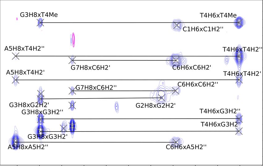
5.5   Thermodynamic properties . . . . . . . . . . . . . . . . . . . . . .   34

6 Discussion                                                                    39
  6.1 The formation of secondary structures . . . . . . . . . . . . . . .       39
  6.2 Comparison of stability with the nearest-neighbor model . . . . .         41
  6.3 Comparison with Tm from previous experimental results . . . . .           41

Conclusion                                                                      43

Bibliography                                                                    44

List of Figures                                                                 47

List of Tables                                                                  50

List of Abbreviations                                                           51

                                        2
Introduction
Nucleic acids in nature achieve a high variety of secondary structures with up
to four strands. Our interest lies in the single-stranded hairpins. Some sequences
create highly stable hairpins with a strong dependence on nucleic base sequences.
Perhaps that is why hairpins are a fairly common pattern in viral RNA[1][2].
The procaryotic replication bubble starts by the spontaneous cruciform for-
mation (or, in other words, the formation of two hairpins) in the procaryotic
replication bubble[3]. Likewise, in transcription, the ends of coding sequences
in procaryotes often form hairpins, which cause the newly-formed RNA strand
to fall off the RNA polymerase.
In humans, hairpin-forming sequences have been found to drive mutation
in triple-repeat error prone regions of the DNA[4]. The presence of hairpins in
the GGGCTA variant of proximal regions of telomeres[5] seems to be behind
some instability of G4 quadruplexes. While we have found plenty of proof for
the formation of hairpins in human DNA, they all seem to have disruptive effect
that harms the organism more often than not. While there have been attempts
to describe the rules by which the stability of a secondary structure is determined,
they provide an estimate, rather than an accurate prediction.
Nuclear magnetic resonance (NMR) experiments are a useful method in this
endeavor. The principle of NMR is vastly different from other spectral methods
used in biophysics, and temperature varied experiments allow a glimpse into
the melting process and thermodynamics of secondary DNA structures. NMR
has its use especially in the realm of short oligonucleotides, where it allows us to
calculate separate thermodynamic parameters for each nucleotide with precision.
The main goal of this thesis is to predict which seven bases long oligonu-
cleotide sequences form stable hairpins, and to assign chemical shifts in selected
DNA strands. Temperature varied NMR experiments will then describe the ther-
modynamic stability of the chosen samples, and we will use those to determine
whether or not do the candidate strands indeed form the predicted hairpins.
31. Deoxyribonucleic acid
The primary structure of deoxyribonucleic acid (DNA) consists of three com-
ponents. The phosphate backbone holds the chain together, the deoxyribose
molecule in each nucleotide is responsible partially for conformation and par-
tially for connecting the backbone and the nitrous base, and the base itself is
the carrier of genetic information. The four major DNA bases, adenine, guanine,
thymine and cytosine, are pictured in Fig. 1.1.
The numbering convention dictates that deoxyribose is labeled with primes
(C1’, C2’, etc.), the nitrous bases are numbered as depicted in Fig. 1.1, and
the nucleotides in a chain are indexed from 5’ end to the 3’ end. The nitrogen
atoms in position 1 in pyrimidines and 9 in purines form a glycosidic bond with
deoxyribose C1’. Each of the bases has 3 exposed edges for hydrogen bonding: the
Watson–Crick edge (named after its role in canonical base pairing), the Hoogsteen
edge (playing its role in an alternative base pairing), and the sugar edge (which
is often sterically blocked from any pairings by the deoxyribose). Fig. 1.1 shows
not only the convention for atom numbering, but also the naming of the edges.
1.1 Conformations of nucleotides
The degrees of freedom in a nucleotide are highlighted by the arrows drawn in
Fig. 1.2. The glycosidic torsion angle χ has its energetic minima in the syn
and anti conformations, with the base either above, or away from the deoxyri-
bose, respectively[6]. These two distinct conformations expose different edges for
potential hydrogen bonding.
The most common sugar puckers of the deoxyribose are 3’-endo, 3’-endo
2’-exo, 2’-endo 3’-exo, and finally, 2’-endo, where the endo carbons appear to
be above the plane of the deoxyribose, and the exo below. The last are rotations
around the bonds of the backbone, denoted by Greek letters α to ζ. All five
dihedral angles of these bonds can rotate and influence the overall shape of the
molecule, although free rotation is sterically blocked by the molecule.
Ab initio calculations on deoxynucleotides[6] have shown that even without
a solvent, a single pyrimidine monophosphate has the lowest energy in the 3’-endo
with the base in syn conformation.The energy difference favouring syn over anti
conformation is even more pronounced in purine monophosphates due to steric
blocking by the phosphate.
4Figure 1.1: The four major bases of DNA. The C-H edge in pyrimidine bases is
sometimes called Hoogsteen edge for the sake of consistency.
5Figure 1.2: A schematic of a mononucleotide with degrees of freedom highlighted
in blue.
Figure 1.3: Watson–Crick canonical base pairing between complementary bases
A·T and C·G
61.2 Secondary structure
The bases of two (or more) strands of DNA form hydrogen bonds, which hold
the strands together. Those bonds usually form along the Watson-Crick edges
(shown in Fig. 1.3), where cytosine pairs with guanine by three hydrogen bonds
and adenine pairs with thymine by two bonds.
Pairs along other edges are common, and even more so in RNA. A nomencla-
ture for the description of non-canonical base-pairing in RNA has been described
by Leontis et al.[7][8], and lends itself well to DNA applications, too.
Another feature that stabilizes the overall secondary and tertiary structure of
DNA is the stacking interaction among the aromatic rings of the bases. This even
further ensures the stability of the resulting structure, as the most energetically
favorable position for a base lies parallel and slightly off-axis to the aromatic ring
of another one.
The secondary structure of the DNA molecule, or a complex of molecules,
depends on the sequence of bases. Double helices, triple helices[9], guanine
quadruplexes[10], hairpins, kissing complexes, and Holliday junctions[11], are just
some of the tertiary structures that appear in nature, each with its own role in
replication, recombination, or the regulation of gene expression.
1.3 DNA duplex
The most common in vivo secondary structure of DNA is B-DNA. Two molecules
running in an anti-parallel direction form a double helix, connected by Watson-
Crick pairing of the hydrophobic bases, protected from the outside environment
by the phosphate backbone. The bases are in anti angle from the deoxyribose,
which has the 3’-endo pucker. While B-DNA is the most common way the nucleic
acid arranges itself in eucaryotic condensed chromatin, the crystalline A-DNA was
the one first observed by Franklin[12]. Z-DNA, the only left-handed double helix,
serves to relieve tension from untwisting DNA undergoing transcription further
along the strand.
7Figure 1.4: Simplified diagram of a 7-member minihairpin. The three bases 3, 4
and 5 form the loop, while the rest forms the base pairs N1·N7 and N2·N6.
1.4 Hairpin formation
Harpins (also stem-loops or hairpin loops) form by intramolecular hydrogen bond-
ing between two regions of the same strand, forming a double-helical stem, and a
loop. The hairpin may be of any length, but the shortest stable observed hairpins
consist of a three bases long loop, and a stable stem from two base pairs. There
is no upper limit to the length of the stem or the loop, provided the stem is stable
enough to support the loop. Even 12 bases long sequences with 3 base pairs in
the stem and 6 bases in the stem can form stable stem-loops[13][14]. An example
hairpin is pictured in Fig. 1.4.
The spontaneous formation of hairpins at the end of the mRNA strand is the
underlying mechanism for termination of transcription in procaryotes. In eucary-
otic DNA, they play a role in triplet expansion mutations[15][16] by increasing
slippage during replication.
Specific seven bases long oligomers have even been reported on. For exam-
ple, the CGGTACG oligomer is the most common sequence on the 21st and
22nd chromosome in humans[17], and has been compared in molecular dynam-
ics experiments with its close relative, GCGTAGC[18]. GCGTACG[19][20] and
GCGAACG[21]have both been reported to form a duplex. Other sequences aid
transcription in some way, one being AGGAACT at the start of a promoter
for a transcription factor[22], and another, AGGCACG, engaging as part of the
TATA box[23].
82. Thermodynamics of processes
in an aqueous solution
2.1 General reaction in an aqueous solution
The general form of a reversible reaction in a dilute aqueous solution is
k
1
aA + bB −
−
↽⇀
−− cC + dD (2.1)
k−1
where capital letters denote the reactants A, B, and the products C, D, and the
miniscule letters denote their respective stoichiometric coefficients. The equilib-
rium constant for such a reaction is then given as
[C]c [D]d
K= (2.2)
[A]a [B]b
the dimension of which depends on the stoichiometric coefficients, and takes the
general form of concentration to the power of a rational number. The temperature
dependence of K is connected to the Gibbs free energy ∆G by the equation
∆G = ∆H − T ∆S (2.3)
where ∆H and ∆S denote the change of enthalpy and entropy, respectively,
and T is absolute temperature.
2.2 Two-state system with hairpin
and single strand
A reaction between a denatured strand S and a hairpin H takes the form of
S−
−H
⇀
↽ (2.4)
where the equilibrium constant follows to be
cH
K= (2.5)
cS
Concentrations can be converted to dimensionless populations, which have
their sum normalized to one. Populations, rather than concentrations, are more
appropriate for the description of chemical exchange in NMR. The total concen-
tration and population of the oligonucleotide in the solution is the sum of the
concentrations (or populations) on both sides,
c0 = cS + cH (2.6)
1 = p0 = pS + pH (2.7)
9The population of the hairpin will then depend on the equilibrium constant,
which itself is dependent on temperature:
K
pH = (2.8)
1+K
To obtain the melting temperature, we will require the van’t Hoff equation
∆G = −RT ln K (2.9)
The melting temperature of a reversible system is defined as a temperature
where half the molecules is in the product state and half in the reactant state,
meaning that K = 1, and the Gibbs free energy ∆G = 0. The melting tempera-
ture Tm of hairpins does not depend on concentration, but only on the enthalpy
∆H and the enthropy ∆S of the reaction:
∆H
Tm = (2.10)
∆S
2.3 Two-state system with duplex
and single strand
For the formation of a duplex D from identical strands S,
2S ⇌ D (2.11)
the equilibrium constant derived from Eq. 2.1 follows to be
cD
K= (2.12)
c2S
Here, the population approach is more useful than the concentration approach.
While the total concentration of oligonucleotide c0 stays the same, the sum of con-
centrations cS and cD no longer equals c0 for any cD > 0. However, populations
always sum up to one. The population approach highlights the fraction of total
molecules, rather than the concentration. The relationships between concentra-
tions and populations are:
cS
pS = (2.13)
c0
cD
pD = 2 (2.14)
c0
The van’t Hoff equation is slightly different from 2.9:
∆G = −RT ln(cref K) (2.15)
The reference concentration cref may be arbitrarily chosen. In this thesis, we
choose 1 M. R represents the universal gas constant. The van’t Hoff equation
linear in ∆H, ∆S is derived from the equations 2.3 and 2.15 as
1 ∆H ∆S
(︃ )︃
ln K = − + (2.16)
cref RT R
10The population of duplexes pD can be calculated from the equations 2.16,
2.12, 2.13,2.14 and 2.15 as
√
1 + κ − 1 + 2κ
pD = , (2.17)
2κ
4c0 −∆G
(︃ )︃
κ= exp (2.18)
cref RT
And finally, the melting temperature can be calculated as
∆H
Tm = (2.19)
∆S − R ln ccref0
2.4 Three-state system with duplex, hairpin,
and single strand
A system which can form both hairpins and duplexes would have the following
set of chemical equations,
2S ⇌ D and S ⇌ H (2.20)
The populations still sum up to one, with their relationship to the concentra-
tions as follows:
cD cS cH
pD = 2 pS = pH = (2.21)
c0 c0 c0
c0 = 2cD + cS + cH (2.22)
1 = pD + pS + pH (2.23)
cD cS cH
1=2 + + (2.24)
c0 c0 c0
The equilibrium constants for this set of equations are then
cD
K1 = (2.25)
c2S
cH
K2 = (2.26)
cS
Together, the equations 2.23, 2.25 and 2.26 with the use of substitutions 2.21
give us the following populations, dependent only on the equilibrium constants
(which themselves depend on the temperature)[24].
√︂
(K2 + 1)2 + 8c0 K1 cref − K2 − 1
pS = (2.27)
4K1 c0 cref
pD = 2K1 c0 p2S (2.28)
pH = p S K 2 (2.29)
11Not only do the thermodynamic parameters give us the required energies that
can be used for further analysis of the processes of replication, transcription and
DNA repair, but the melting temperature calculated can be used to distinguish
among multiple possible secondary structures: the fit of the melting curve and
the change of the melting temperature (or lack of thereof) with c0 are a definitive
proof of the formation of hairpins in the sample.
2.5 Nearest-neighbor model
Prediction of the aforementioned thermodynamic parameters has been attempted
by multiple approaches. The most comprehensive one is the nearest neighbor
model[25] which lies at the core of the DINAMelt[26] web server tool, which
serves to predict the secondary structure of nucleic acids and their properties.
The values for 10 possible variations of nearest neighbors are tabulated. The
Gibbs free energy estimate is calculated as a sum of all nearest neighbor terms
forming a pair, plus penalty for the ending base pair, among other terms. The
nearest neighbor model serves as a good estimate of oligonucleotide secondary
structure stability.
123. Nuclear Magnetic Resonance
Each atomic nucleus has a spin I and posesses a magnetic moment, µ, which
relate to each other through the gyromagnetic ratio γ as
µ = γI. (3.1)
The gyromagnetic ratio is a characteristic value tabulated for every isotope in
its ground state. Examples of some nuclei used in biochemical applications of
magnetic resonance are shown in Table 3.1. Note that the 12 C isotope has been
omitted due to its spin 0.
The spin I has properties of a quantum angular momentum. Each particle
with a spin has 2I + 1 degenerate energy levels. This degeneration is removed by
the presence of a magnetic field, B0 by Zeeman effect. Let us assume a homoge-
nous B0 = (0, 0, B0 ). The difference between two adjacent energy levels in this
magnetic field can be expressed as
∆E = γB0 ℏ. (3.2)
At equilibrium, nuclei within the field B0 are distributed on energy levels
according to the Boltzmann distribution. The sum of magnetic moments of N
nuclei in a given sample, nuclear magnetization M0 , follows from Curie’s law and
the Boltzmann distribution as
N I(I + 1)ℏ2 γ 2
M0 = B0 . (3.3)
3kT
3.1 Bloch equations
The macroscopic nuclear magnetization M interacts with the magnetic field ac-
cording to the Bloch equations:
dMx Mx
= γ(M × B)x − (3.4)
dt T2
dMy My
= γ(M × B)y − (3.5)
dt T2
dMz Mz − M0
= γ(M × B)z − (3.6)
dt T1
where T1 denotes the longitudinal relaxation time, T2 the transversal relaxation
time, and M0 is the equilibrium nuclear magnetization.
Table 3.1: Example isotopes and their respective gyromagnetic ratios[27]
Isotope Spin I γ [106 rads−1 T−1 ] Natural abundance [%]
1
H 1/2 257.522 99.972
2
H 1 41.066 0.015
13
C 1/2 67.273 1.1
14
N 1 19.338 99.6
15
N 1/2 -27.126 0.37
31
P 1/2 108.394 100
133.2 Free induction decay
The simplest pulse-NMR experiment is a hard pulse along the x-axis, which
turns the magnetization vector M by 90◦ from (0, 0, M0 ) to (0, −M0 , 0). After
the pulse, the magnetization vector precesses while relaxing back into M0 . As
the system relaxes back into equilibrium, the longitudal magnetization M∥ builds
back up
− Tt
M∥ = Mz = M0 (1 − e 1 ) (3.7)
and the transverse magnetic relaxation is detected by coil as FID with Larmor
frequency ω0 :
− Tt
M⊥ = M0 e−iω0 t+ϕ e 2 (3.8)
The term eiω0 t in M⊥ (t) in Eq. 3.8 describes precession of the magnetization
around the z axis. If only the static field B0 = (0, 0, B0 ) is present, each of the
nuclei individually undergoes free precession with Larmor frequency, also known
as frequency of the free precession of magnetization. It follows from the Bloch
equations and depends on the magnetic field B0 and the gyromagnetic ratio of
the nucleus,
ω0 = −γB0 (3.9)
The Fourier transform of Eq. 3.8 is the complex spectrum, S(ω), with its
real and imaginary parts being the absorption and the dispersion Lorentz curves,
respectively. The full width at half-maximum for an ideal spectral line is equal to
2/T2 . Faster relaxation therefore leads to line broadening. The following equation
describes the complex lorentzian[27]:
1
L(ω; ω0 , T2 ) = (3.10)
1/T2 + i(ω − ω0 )
Its real part, the absorption lorentzian, follows:
λ
A= (3.11)
(1/T2 )2 + (ω − ω0 )2
All of the above implies that the magnetic field B0 is perfectly homogenous,
which of course cannot be the case. Spectral lines are subject to broadening due
to field gradients. Their T2∗ is shorter than T2 according to the following equation:
1 1
∗
= + γ∆B0 (3.12)
T2 T2
where ∆B0 denotes the difference in the magnetic field strength.
3.3 Chemical shift
The total magnetic field B influencing the Larmor frequency of the nucleus com-
prises from the external field B0 and the shielding by surrounding electrons, which
14is generally a tensor, σij . In liquid samples of low viscosity, only the isotropic
shielding σ determines the spectral shape:
1
σ = Tr(σ). (3.13)
3
The angular resonance frequency of a nucleus with the shielding effect changes
by γσB0 , to
ω = γ(1 − σ)B0 . (3.14)
As the usual difference in 1 H spectra of diamagnetic compounds is in the range
of 10−6 of the original frequency, chemical shift δ is expressed as units of ppm
(parts per million), relative to the frequency of a standard ωs :
ω − ωs
δ= (3.15)
ωs
3.4 Dipole-dipole interaction
The direct dipole-dipole interaction is due to the direct interaction between the
magnetic moments of two nuclei. In isotropic liquids, the rotation of molecules
during experiments time-averages the contribution of dipole-dipole interaction to
zero.
Indirect dipole-dipole interaction, or J-interaction, is propagated by electron
orbitals, introducing the requirement of chemical bonds. This causes a splitting
of a single peak into a multiplet of n + 1 peaks with binomial ratios in case
of n equivalent J-couplings. The number of peaks in the multiplet is equal to
the number of equivalent coupled nuclei plus one, with integrals of said peaks in
binomial ratios to each other. Three-bond J-coupling for 1 H in organic molecules
is approximately 7 Hz.
Both the chemical shift and the multiplicity of a signal from a nucleus can
help in determining its position in a given molecule.
3.4.1 Nuclear Overhauser effect
The Nuclear Overhauser Effect (NOE) is related to the spin-lattice relaxation.
Cross-relaxation between two nuclei is induced by their direct dipole-dipole in-
teraction.
Among other uses, a NOESY experiment with optimal signal build-up can be
used to distinguish between trans and cis isomers of simple organic molecules, or
measurement of inter-proton distances.
NOE does have other applications (most notably, using 1 H cross-relaxation
to enhance peaks in 13 C spectra[27]), but we are most interested in its ability to
show cross-relaxation between two spatially close 1 H nuclei.
3.4.2 2D NOESY
The NOESY sequence, consisting of three 90◦ pulses, the evolution time t1 , and
the mixing time tm , is depicted on Fig. 3.1. A second dimension is introduced
into NMR spectra through the change of a parameter in a set of 1D experiments.
151
H – 1 H NOESY (Nuclear Overhauser Effect SpectroscopY) varies the evolution
time t1 . By applying Fourier transform on the t2 dimension on the resulting free
induction decays (FIDs) we obtain a set of 1D spectra. Transforming these fur-
ther across the t1 dimension results in a 2D spectrum. Off-diagonal crosspeaks at
coordinates (δ1 , δ2 ) can appear for nuclei with chemical shifts δ1 and δ2 , if they
are coupled by a direct spin-spin interaction. Therefore, spatial proximity of two
atoms can be identified. Following up the NOESY sequence with water sup-
pression techniques allows us to obtain 2D spectra with nearly negligible solvent
signal.
90° 90° 90°
t1 tm t2
AQ.
Figure 3.1: NOESY sequence diagram
3.5 Chemical exchange
NMR spectroscopy can be used to observe processes the sample may undergo.
A chemical reaction, or even a conformational change may inadvertently cause
a change in the chemical shift of a particular nucleus. These two different frequen-
cies, ΩA and ΩB result in two distinct spectral lines if the rate constant k of the
process is significantly smaller than their difference Ω∆ , but these spectral lines
draw closer to each other as the system approaches the intermediate exchange
regime at k ≈ Ω∆ , and coalesce to a broad spectral line with high T2∗ . With in-
creasing rate constant (typically from changes in temperature, concentration, or
amount of available enzyme), the process enters the fast exchange regime, result-
ing in a narrow spectral line (Fig. 3.2). The new spectral line has the frequency
of the weighted mean
Ω = Ω A pA + Ω B pB (3.16)
where pA and pB are the populations of the two species.
An S ⇌ H system, as outlined in section 2.2, is an example of chemical
exchange. Assuming that chemical shifts of nuclei in both hairpin and unfolded
state follow linear dependence on temperature, the general form of the dependence
of chemical shift on temperarure under fast chemical exchange can be expressed
as
δ = (aT + b)pH + (cT + d)(1 − pH ). (3.17)
16Figure 3.2: Two-site chemical exchange lineshape is dependent on the rate con-
stant k relative to the angular frequency difference Ω∆ . Reproduction from [27].
Figure 3.3: A demonstration of a generalized sigmoid curve calculated from
Eq. 3.17, with asymptotes (red and yellow) that are not necessarily parallel.
The asymptotes show the chemical shift of the two species if the system did not
undergo chemical exchange.
Note that the 1 − pH term here is equal to pS , as the sum of populations is
always equal to one. An example of such generalized sigmoid curve is provided
in Fig. 3.3.
In a fast chemical exchange of the system in Eq. 2.20, the chemical shifts’
behavior is analogous to the one outlined for hairpins in Eq. 3.17.
δ = (aD T + bD )pD + (aS T + bS )pS + (aH T + bH )pH (3.18)
3.6 Spin echo
If after excitation and a τ /2 delay, 180◦ inversion pulse is applied, the spins
rephase back and a spin–echo signal is observed after a further τ /2 delay. The
echo signal has amplitude multiplied by e−τ /T2 compared to a FID taken right
after the excitation pulse. Spin echo has its use in the refocusing of chemical shift
17Figure 3.4: Comparison of decoupled and undecoupled NMR spectra of 31 P nuclei
of 1.15 mM d(GCGTAGC) at 298 K.
in composite NMR sequences.
3.7 Decoupling
Suppressing the effect of J-coupling can be achieved by continuous irradiation,
or more often composite pulse decoupling, of the coupled nuclei. The result is
a spectrum similar to the non-decoupled spectrum, but with multiplets replaced
by single peaks. Fig. 3.4 demonstrates a comparison between the spectra.
3.8 Solvent suppression
Suppressing the signal of solvent may be desirable in experiments with low solute
concentrations.
3.8.1 Presaturation
In presaturation, the 1 H solvent Larmor frequency is continuously irradiated,
equalizing the populations of its energy levels.
Presaturation also has the effect of completely eliminating the signal of ex-
changeable protons from the NMR spectrum.
3.8.2 Excitation sculpting with gradients
This method, first outlined in 1995[28] as part of the WATERGATE (WATER
suppression by GrAdient Tailored Excitation) family[29], uses a pair of gradient
pulses at the frequency of the solvent 1 H nuclei. The first gradient pulse dephases
the spectrum. It is then followed by a set of pulses that are equivalent to 180◦
pulse for the rest of the sample, but not for the solvent. As a result, the second
gradient pulse refocuses all the spins, except for the solvent.
The equivalent 180◦ pulse is usually done in two ways, represented by the
zgesgp, and zggpw5 sequences on Fig. 3.5. The first is a Gauss pulse tuned to
the suppressed frequency, followed by a hard 180◦ pulse. The second achieves the
same goal with a binomial train of hard pulses, which again sum up to 180◦ . The
other nuclei undergo the same process as they would do in a spin echo, but the
water signal is dephased and suppressed.
18While there are other techniques of solvent suppression, the shortest WATER-
GATE class sequences can achieve that task in a short timespan: that means the
exchangeable protons (in -OH and -NH groups) have lower likelihood of being
exchanged with the solvent in the time between excitation and measurement.
Their signal may be visible with this technique, even if it is completely suppressed
in others.
19Figure 3.5: NMR sequences of interest from Bruker sequence catalog[30]
204. Materials and Methods
4.1 Sample preparation
We prepared two different solutions, which were mixed to achieve pH = 7: one
solution contained Na2 HPO4 , while the second was prepared with NaH2 PO4 .
Solutions included NaCl, so that the concentrations of Na+ would be equal in
both. The resulting buffer solution consisted of 25 mM PO4 3- and 200 mM Na+
in 10% D2 O and 90% H2 O. The NMR standard used was DSS with the IUPAC
name 3-(trimethylsilyl)propane-1-sulfonate. Fully deuterated 0.8µM EDTA was
added to ensure chelation of any unwanted polydentate metal ions.
The DNA oligonucleotides were purchased from the Faculty of Science of
Masaryk University, Brno, Czech Republic, where they were prepared on an Ex-
pedite Nucleic Acid Synthesis System. They were HPLC purified and five times
lyophilized by the producer. These samples were dissolved in the buffer solution
specified above.
Two sequences of DNA which differ by the order of the first two base pairs,
CGGTACG (referred to as Charlie) and GCGTAGC (henceforth referred to as
George) were each dissolved in 0.6 ml of the buffer solution, resulting in approxi-
mately 1 mM solutions of each. The exact concentrations may be found in table
4.1.
4.2 NMR spectroscopy
All spectra were measured on the spectrometer Bruker Avance III HD, with mag-
netic field 11.7 T, which corresponds to the 1 H resonance frequency 500.13 MHz.
The experiments were undertaken with the BBFO probe, a broadband probe
capable of automatic shimming, as well as tuning and matching.
4.2.1 Water suppression optimization
The spectra were measured on a 2.5 mM sample of CTTm5 CGAAG, with pH = 7
buffer solution of 75 mM PO4 3- and 200 mM Na+ with 10% D2 O solvent and
DSS as an internal standard. No EDTA was used in this case. Three pulse
experiment families were investigated: presaturation (zgpr, zggppr, zgcpgppr),
WATERGATE with a single pair of gradients (p3919gp), and WATERGATE
with two pairs of gradients (zgesgp, zggpw5). All experiments were done with
4 scans preceded by 4 dummy scans. The presaturation relaxation delay (D1)
was 3 seconds, and WATERGATE D1 was 1 second.
31
4.2.2 Determination of concentration by P NMR
The concentration was determined from a zg experiment on the 31 P nuclei. 1000
scans (NS) and no dummy scans were taken, each with 2 seconds of acquisition
tome over 16384 points of the time domain (TD). Relaxation delay (D1) was
60 seconds between measurements.
2125.0000
6.8862
2 0 - 2 [ppm]
Figure 4.1: Concentration determination in the George sample from known con-
centration of inorganic phosphate. The oligonucleotide contains 6 phosphates in
its backbone.
Table 4.1: Samples used
sample name DNA sequence concentration
Charlie CGGTACG 1.66 mM
Charlie 0.2 CGGTACG 0.28 mM
George GCGTAGC 1.15 mM
The concentration was then calculated from the ratios of the sum of the area
under phosphate peaks in the DNA backbone, and the inorganic phosphate. A
George 31 P spectrum is shown on Fig. 4.1. The concentrations of the samples
are in the table 4.1
4.2.3 Peak assignment strategy of the aromatic region of
spectra with NOESY
The sequence used for the NOESY spectra, composed of NOESY and water
suppression by excitation sculpting with gradients, can be seen on Fig. 4.2.
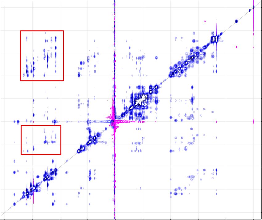
A typical 1 H NOESY spectrum is shown in Fig. 4.3. Two regions, highlighted
here by red rectangles, are of interest. Both of these regions contain crosspeaks
between sugar 1 H nuclei and aromatic 1 H nuclei. The area around 2 ppm is
a region of H2’ and H2” chemical shifts, while the space around 6 ppm contains
mostly H1’. Each of the peaks in the 1D spectrum in the aromatic region (7-
8.5 ppm) of B-DNA, except for the one belonging to the first residue, should
22tm
AQ.
Figure 4.2: Pulse sequence used in peak assignment, noesyesgpph.
have 1 intraresidual H1’ cross-peak and 1 interresidual H1’ cross-peak. The same
applies to H2’ and H2” cross-peaks[31].
The task of assigning the aromatic signals becomes simpler in samples that
have one very distinct nucleus. This is our case in both sequences, where thymine
is represented exactly once. As thymine H6 has a chemical shift between 7.4 and
7.2 ppm, it is alternatively possible to trace in both directions from it, rather than
having to search for the beginning or the ending aromatic atom. The assignment
of the thymine is further supported by crosspeaks to its methyl group, and weak
J-coupling to methyl hydrogens in well-resolved spectra. Moreover, cytosine H6
signals can be easily distinguished from other aromatic atoms, because they form
doublets due to their J-coupling with H6 protons. Adenine H2 signals can be
identified by their missing crosspeaks with deoxyribose in NOESY spectra. As we
didn’t use oligonucleotides with multiple adenines, it wasn’t necessary to develop
a method of discerning among different adenine H2 signals.
4.2.4 Temperature-dependent 1 H spectra
Variable temperature NMR experiments allow us to extract the information about
the stability of the samples. 47 spectra were measured for each sample for the
temperature range 274-366 K, with a step of 2 K. We have used the shortest
possible pulse sequence, namely p3919gp, in order to achieve higher intensity of
broad 1 H signals.
The spectra were obtained at 300 l/h flush gas flow through the probe, and
1200 l/h gas flow through the shim circuit in all temperatures of the sample to
prevent variation. Between measurements at different temperatures, 15 minute
waiting period was inserted to equalize temperature across the sample. Tuning,
matching and shimming were done by automatic procedures right before the
measurements were taken. NS 1024, TD 65536, and D1 1 second for George and
Charlie samples. For the Charlie 02 sample, the NS was increased to 2048.
23Figure 4.3: Charlie at 278 K, an example of a NOESY spectrum of DNA with
suppressed aqueous solvent.
245. Results
5.1 Water suppression sequences
Six pulse sequences in total were examined. The p3919gp (with a full example
spectrum shown on Fig. 5.1) was ultimately chosen due to being an optimal com-
promise between water suppression, amplitude distortion in the water region (Fig.
5.3), and suppression of exchangeable hydrogens (visible on Fig. 5.3 and 5.4).
Furthermore, the short echo time allows superior resolution of hydrogens with
broad signal, such as the one pictured on Fig. 5.2. The trade-off of poor phasing
of the residual water peak in the p3919gp experiment was deemed acceptable, as
we gained the signals of nuclei invisible to slower methods.
5.2 Selection of DNA sequences as hairpin can-
didates
Only oligonucleotides with seven bases, the smallest possible hairpin, were consid-
ered in this thesis. Out of those, the search had to be narrowed even further. The
sequences were chosen according to the following criteria based on canonical base
pairing, in order to minimize the probability of encountering other, undesirable
secondary structures.
• The 1st and 2nd base must be complementary to the 7th and 6th, respec-
tively. That narrows the search to five unique base combinations, resulting
in 45 =1024 possibilities.
• Out of the 1024, 32 candidates (for example, GGATCCC or GGGATCC)
had to be removed from the experiments, as they ran the risk of creating
staggered duplexes instead of the desired hairpin structure.
• 256 sequences with complementary bases in positions 3 and 5 were removed
because they could form stable duplexes with a single mismatch pair.
Figure 5.1: Representative 1D spectrum of an oligonucleotide, taken from the
water suppression experiments with the CTTm5 CGAAG sequence. The amino
hydrogens are distinguished by the change of chemical shift with temperature,
rather than by the region of the shift itself.
25Figure 5.2: The aromatic range of the model 1 H NMR spectrum. While most
peaks far away from water are comparable in all sequences, zgesgp performs worst
in the C1H6 peak at 7.8 ppm. The exchangeable peak at 6.6 ppm is best visible
in the p3919gp sequence.
Figure 5.3: The water region of the NMR 1 H spectra of chosen water suppression
sequences. zgesgp gives us highest sensitivity in the region to the left of the water
peak, all pictured sequences are comparable on the right shoulder of the water
peak. zgcpgppr has the biggest residual water peak.
26Figure 5.4: A significant loss of signal is present in the zgesgp NMR sequence
here: the peak at 2.6 ppm is smaller than in any other sequence class pictured,
and the echo has introduced an antiphase contribution which distorts the baseline
in multiplets.
Even though it fits our criteria, one of the candi-
date sequences, GCGTAGC, has been shown[20] to
form both hairpins and duplexes, showing that the
method is not foolproof. These conditions narrow
the search for suitable candidates down from 1024
to 744. The candidate structures were run through
Figure 5.5: Pairing
the DINAMelt package[26], which revealed that only
between the guanine
31 of them can form stable hairpins above the triple
Watson-Crick edge and
point of water. Judging from the melting tempera-
adenine Hoogsteen edge
tures calculated by the package, the rest is unstable
because an A·T pair in the positions 2 and 6, with its
two hydrogen bonds, doesn’t provide enough structural integrity.
Our goal is not only to predict which 7-member oligonucleotides will form hair-
pins, but also the dependence of their thermodynamic properties on the sequence.
One study[19] scanned through the space of 64 GCNNNGC oligonucleotides by
plotting their resistance towards DNA polymerase against their mobility on poly-
acrylamide gel during electrophoresis, and found that only the ones with GNA
central motif formed stable hairpins.
Structures with the A3-G5 (but not G5-A3) pair were selected against. Pairing
between adenine and guanine would create only a single hydrogen bond, whereas
the pairing between guanine and adenine creates two as per Fig. 5.5. Molecular
dynamics[32] have shown that the bend in the GNA triplet is realized by stacking
of the center nucleotide on guanine.
DINAMelt was unable to calculate the differences in the fourth position in the
oligonucleotide, but it did show a mild preference for purine-pyrimidine stacking.
Experiments on longer sequences[33], however, show preference for hairpins with
the central motive GYA (GCA or CTA), and for duplexes with GRA (GGA,
GAA). Overall, a GNA triplet is a necessary condition for short hairpins.
27Table 5.1: A complete list of heptanucleotides capable of forming hairpins
AGGAACT TGGAACA CCGAAGG GGGAACC
AGGGACT TGGGACA CCGGAGG GGGGACC
AGGCACT TGGCACA CCGCAGG GGGCACC
AGGTACT TGGTACA CCGTAGG
ACGAAGT TCGAAGA CGGAACG GCGAAGC
ACGGAGT TCGGAGA CGGGACG GCGGAGC
ACGCAGT TCGCAGA CGGCACG GCGCAGC
ACGTAGT TCGTAGA CGGTACG GCGTAGC
This results in the 31 candidate structures in table 5.1. Note that the sequence
GGGTACC is omitted, because it can form a staggered duplex.
In the end, we selected two sequences with the central GTA loop, with the
closing base pairs C·G due to their high predicted stabily. The two sequences,
CGGTACG and GCGTAGC, used in this work allow the study of the effect of
the stem on the overall hairpin properties.
5.3 Resonance assignment
We measured NOESY spectra for both samples at 288 K. This was sufficient
for peak assignment in the aromatic region of the George sample. Fig. 5.6
depicts the assignment in the H1’ region, and Fig. 5.7 depicts the assignment in
the H2’/H2” that was done to fill in the gaps and help with the assignment of
guanine aromatics.
However, the 288 K NOESY alone wasn’t sufficient for clear assignment in
the Charlie oligonucleotide. Fig. 5.8 shows the presence of too many crosspeaks,
hinting at a second structure and obscuring the NOESY spectrum of the desired
hairpin. Two more NOESY experiments were needed for unambiguous assign-
ment: a spectrum at 298 K (depicted on Figs. 5.9 and 5.10) provided most
crosspeaks, but left some uncertainty in cytosines, which weren’t resolved enough
at that temperature. A 316 K spectrum didn’t have many peaks remaining, but
it ultimately helped resolve the difference between cytosine aromatic nuclei C1H6
and C6H6 (Fig. 5.11).
It can be shown in the NOESY spectra that the secondary structures are more
likely hairpins than B-DNA duplexes. The crosspeaks between A5H8 and T4H1’,
T4H2’, and T4H2” for both Georgeand Charlieare weaker than other crosspeaks
between an aromatic hydrogen and the deoxyribose from the previous residue. In
B-DNA, the same part of the molecule would be much more rigid, and the same
peaks more clearly resolved.
Now we have a complete aromatic assignment for both oligonucleotides that
we will use further in the melting analysis.
28Figure 5.6: George (GCGTAGC) NOESY at 288 K. Note the missing A5H1’
crosspeaks with A5H8 and G6H8: their chemical shifts are too close to each
other at this temperature for any decisive crosspeaks.
Figure 5.7: George NOESY at 288 K in the H2’ and H2” region. Lines connecting
crosspeaks with the same shift in one dimension have been omitted for clarity.
The missing crosspeaks between the A5 and the G6 residue are a consequence of
the close chemical shifts of the aromatic nuclei.
29Figure 5.8: Charlie (CGGTACG) NOESY at 278 K in the H2’ and H2” region.
16 groups of signals along the aromatic x axis show that there is slow exchange
between hairpin, and another secondary structure with broad peaks.
Figure 5.9: Charlie NOESY at 298 K in the H2’ and H2” region with assignments.
The C1H6 and the C6H6 peaks overlap.
30Figure 5.10: Charlie (CGGTACG) NOESY at 298 K in the H1’ region. The
missing broad peaks of G2H8, and the overlap of C1H6 and C6H6 aromatic shifts
limit the possibility of assignments from this region of the NOESY spectrum.
Figure 5.11: Charlie NOESY at 316 K in the H1’ region, used to differentiate
between the C6H6 and the C1H6 chemical shifts.
31Figure 5.12: Temperature series for the George sample in the aromatic region of
the NMR spectra
5.4 Temperature dependent spectra
The George sample was measured at a single concentration of 1.15 mM. Its tem-
perature series is pictured in Fig. 5.12. Each of the 47 spectra was fitted to
a linear combination of Lorentz curves. The Charlie sample was initially mea-
sured at a concentration of 1.66 mM (Fig. 5.13). This variable temperature series
achieved slow chemical exchange between a hairpin and an unknown secondary
structure up until 292 K. To differentiate the effect of the hairpins from the effect
of possible complexes of multiple molecules, a second series of NMR experiments
at a concentration of 0.28 mM was also included (Fig. 5.14). The tracing of
the fast exchange peaks was therefore done separately for each of the two sets of
peaks. The hairpin and the other set of peaks (that was assumed to be a duplex)
could be distinguished both by the continuity of the tracing of the peaks across
the spectra, and the lower amplitude and broader peaks of the complex. The
result was fitted to a sum of Lorentz peaks with the help of the Asymexfit[34]
package.
32Figure 5.13: Temperature series for the Charlie sample in the aromatic region of
the NMR spectra
Figure 5.14: Temperature series for the Charlie 0.2 sample in the aromatic region
of the NMR spectra
33Table 5.2: Thermodynamic parameters for each nucleus
∆H ∆S ∆G310K Tm
kJ · mol −1
J · mol · K
−1 −1 kJ · mol−1 K
Charlie - CGGTACG at 1.66 mM
C1H6 -57 ± 32 -193 ± 55 3 ± 36 294 ± 162
G2H8 -90 ± 4 -283 ± 10 -2 ± 5 317 ± 2
G3H8 -87 ± 3 -275 ± 10 -2 ± 5 316 ± 2
T4H6 -90 ± 9 -285 ± 29 -2 ± 13 316 ± 2
A5H2 -88 ± 14 -286 ± 37 1 ± 18 307 ± 13
A5H8 -92 ± 9 -291 ± 26 -2 ± 12 318 ± 2
C6H6 -83 ± 7 -262 ± 22 -2 ± 10 316 ± 2
G7H8 -102 ± 142 -326 ± 472 -1 ± 204 312 ± 27
Charlie 02 - CGGTACG at 0.25 mM
C1H6 -84 ± 47 -261 ± 143 -3 ± 65 321 ± 7
G2H8 -89 ±4 -281 ± 12 -2 ± 6 316 ± 2
G3H8 -81 ±4 -256 ± 12 -2 ± 5 319 ± 1
T4H6 -84 ± 23 -269 ± 68 -1 ± 31 313 ± 7
A5H2 -31 ± 126 -107 ± 353 2 ± 167 289 ± 234
A5H8 -91 ± 12 -289 ± 34 -2 ± 16 315 ± 3
C6H6 -76 ± 16 -241 ± 49 -1 ± 22 315 ± 5
G7H8 -38 ± 76 -110 ± 182 -4 ± 95 343 ± 484
George - GCGTAGC at 1.15 mM
G1H8 -52 ± 4 -150 ± 13 -6 ± 6 358 ± 15
C2H6 -100 ± 1 -292 ± 5 -9 ± 2 341 ± 0
G3H8 -103 ± 3 -303 ± 8 -9 ± 4 341 ± 1
T4H6 -100 ± 3 -294 ± 10 -9 ± 5 341 ± 1
A5H2 -94 ± 7 -276 ± 22 -8 ± 10 340 ± 1
A5H8 -97 ± 3 -284 ± 8 -9 ± 4 341 ± 1
G6H8 -67 ± 3 -195 ± 11 -7 ± 5 346 ± 3
C7H6 -115 ± 3 -338 ± 10 -10 ± 5 341 ± 1
5.5 Thermodynamic properties
The chemical shifts of aromatic protons with respect to temperature, obtained in
the previous part, were then fitted by the melting curve according to Eq. 3.17.
Linewidths served as error estimates of the shifts and were used in the fit as
weights. The results are shown in Figs. 5.15, 5.16, and 5.17. Thanks to that
we obtained a set of thermodynamic parameters ∆H, ∆S, ∆G, Tm in Table
5.2 and their errors, for each nucleus. Judged separately, they seem arbitrary.
Together, they show us a picture of the melting process. Graphs 5.19 and 5.18
reveal that the melting temperatures do not vary significantly along the length
of our hairpins.
34(a) G1H8 (b) C2H6
(c) G3H8 (d) T4H6
(e) A5H2 (f) A5H8
(g) G6H8 (h) C7H6
Figure 5.15: Plots of chemical shift against temperature for the aromatic 1 H
nuclei in the George sample, together with a fit curve for each.
35(a) C1H6 (b) G2H8
(c) G3H8 (d) T4H6
(e) A5H2 (f) A5H8
(g) C6H6 (h) G7H8
Figure 5.16: Plots of chemical shift against temperature for the aromatic 1 H
nuclei in the Charlie sample, together with a fit curve for each.
36(a) C1H6 (b) G2H8
(c) G3H8 (d) T4H6
(e) A5H2 (f) A5H8
(g) C6H6 (h) G7H8
Figure 5.17: Plots of chemical shift against temperature for the aromatic 1 H
nuclei in the Charlie 0.2 sample, together with a fit curve for each.
37Figure 5.18: Melting temperatures obtained for each aromatic 1 H nucleus in the
George sample. The nuclei where the fit wasn’t possible are not included.
Figure 5.19: Melting temperatures obtained for each aromatic 1 H nucleus in the
Charlie sample for both concentrations. The nuclei where the fit wasn’t possible
are not included.
386. Discussion
6.1 The formation of secondary structures
The Charlie oligonucleotide was measured at two different concentrations. At
each of these concentrations, the melting temperature Tm was determined for
each nucleus from variable temperature NMR. The consensus melting tempera-
ture is 44 ◦ C in both concentrations, with a uniform melting profile along the
strand. Because the melting temperature doesn’t depend on concentration, the
secondary structure is unimolecular. A comparison between the melting curves
of two example nuclei in both concentration is provided in Fig. 6.1. Comparison
of χ2 for a hairpin model and a duplex model favors the hairpin. A plot of fit
residues is shown in Fig. 6.4.
The Charlie strand has been observed by us to also form a secondary struc-
ture, as shown by the presence of 16 distinct peaks up until 288 K. One such
spectrum is pictured in Fig. 6.2. This secondary structure might be a duplex,
with a drastically lower Tm , as it entirely disappears at lower concentrations. As
was the case in the previous oligonucleotide, chi2 favors the hairpin over duplex.
We measured the George sample at a single concentration, which alone was
sufficient in determining the formation of hairpin with a uniform melting tem-
perature of 68◦ C along the whole strand. A second most likely option was the
formation of duplexes, which was disproven by obtaining thermodynamic param-
eters with an assumption of a duplex (Fig. 6.3). Comparison of χ2 for the duplex
model and for the hairpin model favors the hairpin.
Literature reports a duplex formation within the George strand[20] in 5.7
mM solution. No reference to hairpin and duplex formation was found for the
Charlie oligonucleotide sequence. We haven’t observed George duplex due to the
abnormal stability of its hairpin, and the apparent higher concentrations required
for duplex formation.
Therefore, Charlie and George both form stable hairpins.
Figure 6.1: Comparison of the melting curves of two different nuclei in both
concentrations measured for the Charlie sample. The melting temperature Tm
remains unchanged, because the structure observed is a hairpin.
39Figure 6.2: The aromatic segment of a Charlie NMR spectrum at 278 K. The
broad signals of the duplex are easily discernible from the peaks of the hairpin.
Figure 6.3: Comparison of melting curve fit residues in a model that assumes
the formation of a hairpin (blue) and the formation of a duplex (orange) in the
George sequence.
Figure 6.4: Comparison of melting curve fit residues in a model that assumes
the formation of a hairpin (blue) and the formation of a duplex (orange) in the
Charlie sequence.
406.2 Comparison of stability with the nearest-
neighbor model
Both our measurements and the nearest-neighbor model agree that the melt-
ing temperature of Charlie is lower than the melting temperature of George.
The model’s parameters[25] and the experimental evidence[35] point towards the
stacking of alternating purines and pyrimidines (such as the GCG motif of George)
resulting in more stable structures than stacking without alternating (as is the
case in the Charlie sequence with its CGG stem motif). The nearest-neighbor
energy difference for the 5A-6G in George and 5A-6C in Charlie is smaller than
the difference between 2C-3G (Charlie) and 2G-3G (George), which is why the
second term is a more decisive factor in the stability of the hairpin, and the
Charlie strand melts at lower temperatures than the Georgestrand.
The nearest-neighbor model[26] predicts a 54◦ C melting temperature for Char-
lie (instead of the 44 ◦ C measured) and 58◦ C for George (instead of 68◦ C). The
experiments have successfully shown that the existing models provide qualitative
prediction for the creation of hairpins. The accuracy of these melting temper-
atures, however, is only 10 Kelvin. As the model predicts the same melting
temperatures for oligonucleotides which differ by the central nucleotide in the
loop, the discrepancy can be expected to be even larger for more stable hairpin
loops than the GTA triplet in Charlie and George.
The difference between the model and the experiment can be explained by
the limitations of the nearest neighbor model outlined in 1998[25], which only
accounts for hydrogen bonded pairs, and assigns a flat penalty for unbound bases.
Terms for stacking of the unbound nucleotides with bound ones are not included
in the nearest-neighbor model.
6.3 Comparison with Tm from previous experi-
mental results
While they were not involved in the experimental part of this thesis, other, similar
oligonucleotides are part of the broader scope of understanding of the formation
of hairpins. Table 6.1 depicts results of two teams with the GCGNAGC[36][19]
family of oligonucleotides. It shows an 8◦ C difference between the least stable
chain and the most stable one. While they are consistent with each other, there is
a small difference between their Tm and ours, likely arising from a different buffer
formula. However, it hints at a trend that could be present in all NNGNANN
hairpin candidates. As no melting temperature data for other minihairpins than
the ones mentioned in Table 6.1 is available, this area remains mostly unexplored.
41Table 6.1: Comparison of relevant oligonucleotides Tm .
Rosemeyer, 2004[36] Yoshizawa, 1997[19] this thesis
GCGAAGC 72 72.3
GCGGAGC 71 70.5
GCGCAGC 67 67
GCGTAGC 66 66.3 68
CGGTACG 43
42Conclusion
The aim of this thesis was to evaluate the formation of stable mini-hairpins by
NMR variable temperature experiments. This was done by assessing the candi-
date mini-hairpin sequences by a nearest-neighbor theoretical model, and com-
paring the prediction with experimentally obtained thermodynamic parameters.
• 31 DNA strands forming stable minihairpins were selected with the aid of
the nearest-neighbor model out of a pool of 1024 possible candidates.
• Two sequences, CGGTACG (referred to as Charlie in the thesis) and GCG-
TAGC (referred to as George) which differ only by the order of the first two
base pairs were chosen for measurement.
• We measured NOESY spectra of these two speciments for signal assignment.
• Once assigned, the peaks in the aromatic region were measured across
a range of temperatures from 274 K to 266 K.
• Melting curves were obtained from the 1D spectra by extracting data about
chemical shifts and spectral line widths from the temperature series.
• The thermodynamic parameters of the aromatic nuclei were obtained, giv-
ing us information about the stability and melting temperatures.
We have been able to show that the two selected candidate structures, George
and Charlie, do indeed form stable hairpins. As per the theoretical prediction,
their melting temperatures Tm are vastly different from each other due to the
stabilizing effect of stacking alternating purine and pyrimidine bases in George
(in the form of the GCGNNGC motif), resulting in a 25 K melting temperature
difference between the two. The melting temperature is uniform along the whole
strand for both hairpins. The obtained Tm differ from the model in opposite
directions, suggesting that some other interactions, not included in the nearest
neighbor model, are at play.
43Bibliography
[1] A Roulston, P Beauparlant, N Rice, and J Hiscott. Chronic human immun-
odeficiency virus type 1 infection stimulates distinct NF-kappa B/rel DNA
binding activities in myelomonoblastic cells. Journal of Virology, 67(9), 1993.
[2] Hasan Uludağ, Kylie Parent, Hamidreza Montazeri Aliabadi, and Azita Had-
dadi. Prospects for RNAi Therapy of COVID-19, 2020.
[3] David Bikard, Céline Loot, Zeynep Baharoglu, and Didier Mazel. Folded
DNA in Action: Hairpin Formation and Biological Functions in Prokaryotes.
Microbiology and Molecular Biology Reviews, 74(4):570–588, 2010.
[4] Libuše Trnková, Irena Postbieglová, and Miroslav Holik. Electroanalytical
determination of d(GCGAAGC) hairpin. Bioelectrochemistry, 63(1-2):25–30,
jun 2004.
[5] Jean Chatain, Alain Blond, Anh Tuân Phan, Carole Saintomé, and Patrizia
Alberti. GGGCTA repeats can fold into hairpins poorly unfolded by repli-
cation protein A: a possible origin of the length-dependent instability of
GGGCTA variant repeats in human telomeres. Nucleic Acids Research, jul
2021.
[6] Nicolas Foloppe, Brigitte Hartmann, Lennart Nilsson, and Alexander D.
MacKerell. Intrinsic conformational energetics associated with the glyco-
syl torsion in DNA: A quantum mechanical study. Biophysical Journal,
82(3):1554–1569, mar 2002.
[7] Neocles B. Leontis and Eric Westhof. Geometric nomenclature and classifi-
cation of rna base pairs. RNA, 7(4):499–512, 2001.
[8] Neocles B. Leontis, Jesse Stombaugh, and Eric Westhof. The non-
Watson–Crick base pairs and their associated isostericity matrices. Nucleic
Acids Research, 30(16):3497–3531, 08 2002.
[9] V. Kumar, V. Kesavan, and K. V. Gothelf. Highly stable triple helix for-
mation by homopyrimidine (l)-acyclic threoninol nucleic acids with single
stranded DNA and RNA". Organic & Biomolecular Chemistry, 13(8):2366–
2374, 2015.
[10] Wesley I. Sundquist and Aaron Klug. Telomeric DNA dimerizes by formation
of guanine tetrads between hairpin loops. Nature, 342(6251), 1989.
[11] D. M.J. Lilley. Structures of helical junctions in nucleic acids, may 2000.
[12] R. E. Franklin and R. G. Gosling. The structure of sodium thymonucleate
fibres. I. The influence of water content. Acta Crystallographica, 6(8–9):673–
677, 1953.
[13] O. Socha. Charakterizase strukturních vlastností a stability DNA vlásenek
pomocí NMR spektroskopie. Diploma thesis, Charles University, 2016.
44You can also read