Winners and losers in industrial policy 2.0 - WIDER Working Paper 2020/21 Mohamed Ali Marouani1 and Michelle Marshalian2 - unu-wider
←
→
Page content transcription
If your browser does not render page correctly, please read the page content below
WIDER Working Paper 2020/21

Winners and losers in industrial policy 2.0

Mohamed Ali Marouani1 and Michelle Marshalian2

March 2020
Abstract: Large-scale business subsidies tied to national industrial development promotion
programmes are notoriously difficult to study and are often inseparable from the political
economy of large government programmes. We use the Tunisian national firm registry panel
database, data on treated firms, and a perceptions survey administered by the National Research
Institute to measure the impact of Tunisia’s Industrial Upgrading Program. Using inverse
propensity score re-weighted differences-in-differences regressions, we find that small treated
firms hire more and higher-skilled labour. In small firms, wages increase 10–17 per cent, with
growth in employment and net job creation. However, in larger firms the programme does not
support labour and wages fall, suggesting that there are no benefits to labour when funds go to
large firms.
Key words: firm subsidies, fiscal policy, industrial policy, firm size, impact analysis, labour
JEL classification: H2, O1, L2, O2
Acknowledgements: We would like to thank Leila Bagdadi, Stijn Broecke, Philippe DeVreyer,
Ishac Diwan, Stefan Hertog, Adeel Malik, El Mouhoub Mouhoud, Daniela Scur, Bob Rijkers,
Steve Bond, Julien Gourdon, and Phuong Le Minh for feedback and reviews; workshop inputs
and funding from the Economic Research Forum, Cairo, Egypt; participants at the 2019 Centre
for Studies of African Economies (CSAE) Conference, Oxford; participants at the UNU-
WIDER Development Economics conference in Bangkok (2019); participants at the
ASSA/MEEA meetings in San Diego (2019); Hassen Arouri, Rim Chabbeh, and Mohamed
Hammami, Institut Nationale de la Statisique (INS-Tunisia); Zouhair Elkadhi, Director General,
Institut Tunisien de la Competitivité et des études Quantitatives (ITCEQ). This work was
supported by the Economic Research Forum, in Cairo. A previous version of this paper has
been published in the working paper series of the Economic Research Forum (Marouani and
Marshalian 2019). All opinions and errors are our own.

1 UMR Développement et sociétés, IRD, Paris, France; Paris 1 Pantheon-Sorbonne University, Paris, France; Economic

Research Forum, Tunis, Tunisia; 2 University of Paris, Dauphine (PSL), Paris, France; Paris 1 Pantheon-Sorbonne University,
Paris, France; DIAL, Paris, France; corresponding author: Michelle-lisa.Marshalian@univ-paris1.fr
This study has been prepared within the UNU-WIDER project Varieties of structural transformation.
Copyright © The Authors 2020
Information and requests: publications@wider.unu.edu
ISSN 1798-7237 ISBN 978-92-9256-778-1
https://doi.org/10.35188/UNU-WIDER/2020/778-1
Typescript prepared by Gary Smith.
The United Nations University World Institute for Development Economics Research provides economic analysis and policy
advice with the aim of promoting sustainable and equitable development. The Institute began operations in 1985 in Helsinki,
Finland, as the first research and training centre of the United Nations University. Today it is a unique blend of think tank,
research institute, and UN agency—providing a range of services from policy advice to governments as well as freely available
original research.
The Institute is funded through income from an endowment fund with additional contributions to its work programme from
Finland, Sweden, and the United Kingdom as well as earmarked contributions for specific projects from a variety of donors.
Katajanokanlaituri 6 B, 00160 Helsinki, Finland
The views expressed in this paper are those of the author(s), and do not necessarily reflect the views of the Institute or the
United Nations University, nor the programme/project donors.

1          Introduction

Industrial policy has long lost favour in light of difficulties regarding the effectiveness and political
economy of structural adjustment programmes. The unpopularity of industrial policy grew from its
capacity to produce and exacerbate market distortions, as well as the fear of political capture of subsidies
in developing countries (Rodrik 2008). However, little differentiates the failures of these types of policies
from the failures in long-entrenched and accepted ‘horizontal’ policies, such as those that subsidize
education or health services.1

Despite concerns and common pitfalls, industrial policy remains a common intervention for govern-
ments. Initiatives targeting industrial development2 are often used to stimulate growth and employment.
At the same time, they have unrevealed political economy ramifications, particularly in authoritarian
regimes where the emergence of a robust private sector is considered a threat to state power and control
of rents (Cammett 2007; Malik and Awadallah 2013; Rougier 2016). The state guarantees its clients a
non-competitive environment and endogenous regulation protecting their interests (Rijkers et al. 2017).
An example of one such policy is the Tunisian Industrial Upgrading Program (IUP) implemented in the
1990s to facilitate the country’s integration into the world economy.

The literature on firm subsidies suggests that this type of industrial policy can have a positive impact
on jobs and output (Bernini et al. 2017; Criscuolo et al. 2019; Einiö 2014), even if this is not always
the case for all types of subsidies (Wallsten 2000). Other studies find evidence that positive change in
total factor productivity is only captured in the long run, if at all (Bernini et al. 2017; Criscuolo et al.
2019; Einiö 2014). According to Wallsten (2000), firm-level investment subsidies crowd-out self-raised
investments. On the other hand, Einiö (2014) finds no evidence of crowding out, and McKenzie et al.
(2017) find a positive impact on capital investments and innovations. Furthermore, most studies report
finding an anticipation effect before treatment, changes in behaviour during the treatment period, and
varying impacts by the type of subsidy received (Bernini et al. 2017; Criscuolo et al. 2019; Hottenrott
et al. 2017; Wallsten 2000). The objective of this paper is to contribute to this literature through two
main avenues. First, we investigate how firm subsidies impact labour and wages over time in large-scale
programmes with staggered treatments. Second, we explore whether the effects are heterogeneous by
firm size.

This paper is the first impact evaluation of a large-scale industrial programme in the Middle East and
North Africa, and a rare example in developing countries. The size and coverage of these programmes
often involve a roll-out of programme implementation over time (De Janvry and Sadoulet 2015). Our
identification strategy is based on non-perfect identifiers, similar to the identification strategy used by
Criscuolo et al. (2019).3 Once we identify firms, we use a weighted propensity score matching method to
create control groups and extended the analysis with a fixed effects differences-in-differences regression

1 ‘Horizontal’ policies can impact all sectors, and do not necessarily have a sector-specific component. Nevertheless, they can
impact some sectors differently than others. For example, the protection of business and labour interest groups, or education,
training, or health-related policies, are ‘horizontal’ industrial policies. However, ‘horizontal’ policies such as training and
education are not ‘sector-blind’. They are economy-wide but impact some sectors more than others. For example, focusing
on technical computer skills training will not help manufacturing production lines as much as it will provide skilled labour
for services. On the other hand, ‘Vertical’ industrial policies have a sector- or firm-specific component and can target entire
sectors or firms within sectors. Vertical industrial policies can include, for example, policies specifically for tradable sectors
or business subsidies or interest rate reductions targeting one type of sector or economic activity. In the context of developing
countries, political capture occurs as frequently in the basic social welfare, or ‘horizontal’ policies, as in business subsidies
and ‘vertical’ policies.
2   We focus here on firm subsidy programmes as one type of major industrial policy.
3 In this paper we provide an additional robustness test on the credibility of our identification strategy, and restrict the analysis
to where we have a higher level of sureness in our identification strategy.

                                                                 1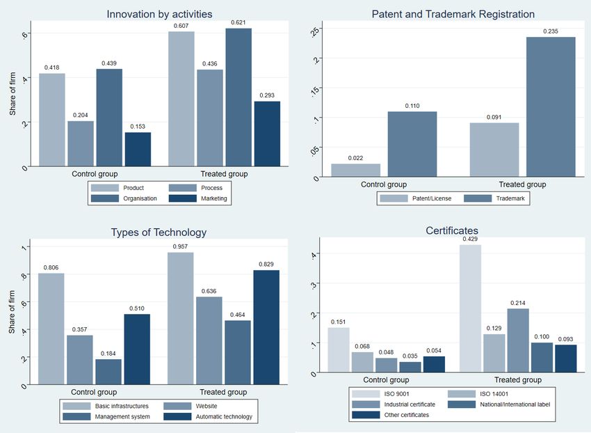
analysis (Cadot et al. 2015; Hirano et al. 2003). Similar multiple treatment studies use basic matching
techniques or more aggregate synthetic control group methods. This approach is analytically similar to
the synthetic control group method with a differences-in-differences regression, except by following the
Hirano et al. (2003) approach, we keep the possibility of firm-level analysis.

As a first result, the fixed effects ordinary least squares (OLS) estimates suggest that the programme
increased overall employment and wages. However, the effect on employment was not robust to the
inclusion of controls and regression readjustment, suggesting that on an aggregate level, the programme
did not increase employment, and that this positive impact was due to selection bias. On a more dis-
aggregate level, employment and wages grew in small firms. In our full model, we observed increases in
net job creation in smaller firms. The estimates suggest that in small firms workers retained some of the
benefits of this programme because they gained in jobs and job quality. Inversely, there is little evidence
of wage growth in large firms, but more often significant drops in wages. The decrease in wages is
observed jointly with the losses in employment. This observation on wages and employment suggests
that, in large firms, there was a substitution of labour. This finding suggests that it is likely that capital
owners retained the benefits from the programme. We conclude that this programme’s political purpose
is welfare-enhancing in small firms, but clientelism in larger firms.

The rest of the paper (1) describes the Tunisian upgrading programme; (2) provides a data description;
(3) proposes an identification strategy and econometric approach; (4) discusses the descriptive analysis,
regression results, and robustness and sensitivity tests; and finally (5) discusses the results within the
political-economy context of Tunisia.

2        The Tunisian Industrial Upgrading Program

The Tunisian IUP, implemented in anticipation of full entry into the free trade agreement with the Eu-
ropean Union, initially aimed at bringing the competitiveness of firms to a comparable level after the
Multi-Fiber Arrangement for textiles and before the EU free trade agreements (Cammett 2007). At the
time of entering the free trade agreement, Tunisia requested additional time and financial assistance to
support structural adjustment and competitiveness.

The IUP was initially limited to the manufacturing sector. However, in 1997, services with strong
links to manufacturing were added to the list of beneficiary sectors. More than 5,000 grants have been
distributed in the last 20 years, corresponding to a total amount of TND1,260 million (Tunisian dinars;
around US$500 million). Two-thirds of the amount was spent on material purchases and the rest on
immaterial acquisitions (Ben Khalifa 2017).4 The bureau of the IUP prioritized material investment
initiatives that improved product conception, research and development, and laboratory equipment, and
immaterial investments that improved productivity and quality of products, the development of new
products, and costs related to hiring higher-educated managers (Amara 2016).5

4 Material investments included technical equipment for management, research and development, and quality-control pur-
poses. These could be targeted at modernizing production equipment, adopting new technologies, diversifying the production
of goods, integration of new processes in the production cycle, maintenance, and installation of basic utilities (for example,
production chemicals, electricity). Immaterial investments included computer programs and technical assistance (in the up-
grading of the productivity within the production process), consulting services, financial advisory, technology transfer, and
support in the acquisition of patents and licences.
5 Like in the Yemeni firm subsidy matching initiative (McKenzie et al. 2017), when the IUP provided material investment
support, it required at least some cost matching by firms, and subsidized up to 70 per cent of immaterial expenses up to a
ceiling.

                                                              2
The qualification conditions for the IUP are rather straightforward. Firms need at least two years of for-
mal registration (incorporation) and, critically, they need to belong to eligible industries, which include
the following: agriculture and food; construction; ceramics and glass; chemicals; textiles, clothing, and
leather; mechanical, metal, and electrical work; and diverse industries such as services related to these
activities. Inherently, it also required firms to be in the formal market, and that firm fiscal accounts were
up to date and legible by the selection committee. According to Murphy (2006), firms wishing to benefit
from the programme made an initial application that responded to a set of principles and objectives,
rather than a standard application form.6 If accepted, firms are asked to provide a strategic and financial
diagnostic. Technical support was then provided by either technical centres, the Agence de Promotion
de l’Industrie for public–private partnerships, or private firms.7
Most firms that applied received funding.8 The average funds per applicant9 was higher in the north-
eastern region (Figure 1, Panel A). However, in the last 20 years (1996 to mid-2017), the distribution of
total funds for the IUP has been primarily concentrated in the northern coastal regions (Figure 1, Panel
B and Appendix Figure A1). Over the entire period of funding, 17 per cent of total funds for the IUP
went to the region of Ben Arous. The region of Nabeul received 13 per cent of all funds, and the regions
of Monastir, Sfax, and Sousse each received 11 per cent of the total funding pool. The relatively higher
approval-to-applicant ratio in the north and eastern coasts (Figure A1, Panel D) was also reflected in the
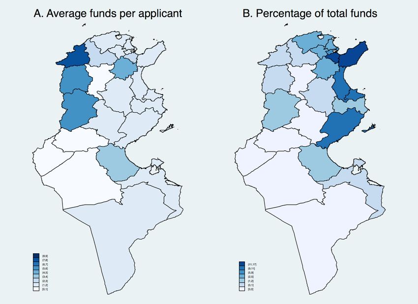
fact that fewer firms applied in those regions (Figure A1, Panel B).10
Figure 1: Distribution of IUP funds by region
Note: Rates are weighed by total applicants per region. Total and average funds are in current millions of TND.
Source: Authors’ compilation, based on data from the Bureau de Mise à Niveau.
6 This was also the case in the firm matching subsidy programme in Yemen (McKenzie et al. 2017).
7 Further information on the decision to select firms was unfortunately not available for this research.
8 The fact that firms had to apply to receive funding also means that there is implicit selection bias before firms applied. Firms
that applied likely have different observable and non-observable characteristics from those that did not.
9 Average funds per applicant are weighed by total applicants per region.
10 This was weighted by total applicants per region.
3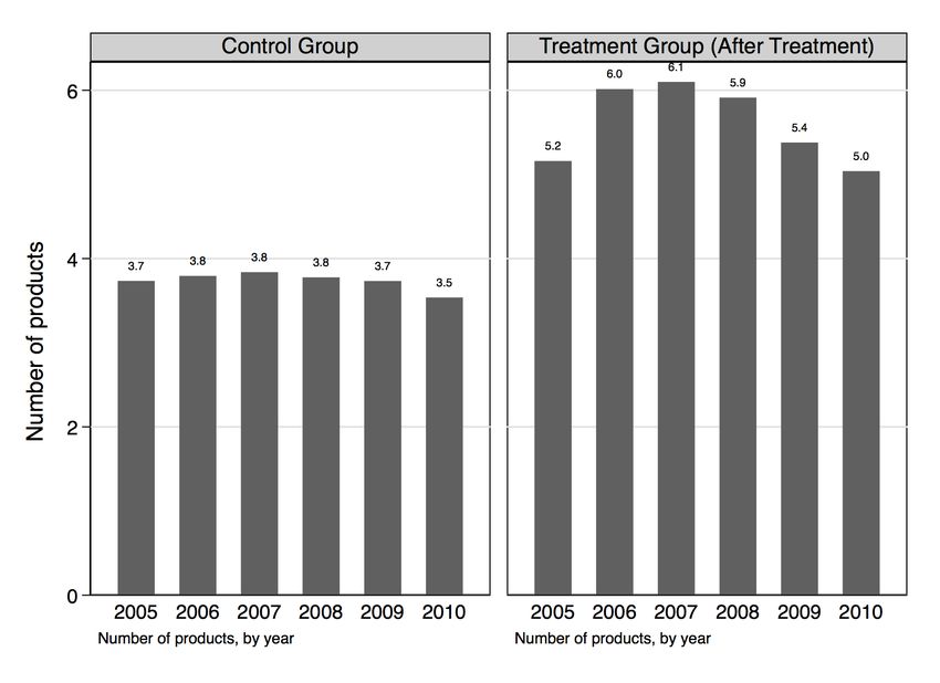
3         Data description

The primary source of our paper is from the national firm-level enterprise registry (Répertoire nationale
des entreprises, RNE) administered by the National Statistical Institute (l’Institut national de la statis-
tique, INS). It includes data for all formal firms for 18 years, from 2000 to 2017, with close to four
million observations. This resource is the most exhaustive source for firm-level data in Tunisia. The
database is linked with business turnover, profits, and firm-level employment data from the Ministry
of Finance. It was also possible to link the data directly with the national export–import customs
database, including export values and volumes on the HS6 product level and by country (for years
2005 to 2010).

For our analytical purposes, we use a sub-sample of firms that had six or more employees in at least
one period in the database. The use of this sub-sample means that firms with fewer than six employees
at time t may exist as long as the firm had at least six employees at some point in the 18 years of data
available in the RNE. The reason for the restriction on the size of firms is two-fold. First, the quality of
the data collected for firms with fewer than six employees is low. Second, and more importantly, only
firms with six or more employees are required to file taxes and can therefore benefit from government
subsidies and tax breaks. Firms with fewer than six employees are often informal and do not benefit from
the same financial incentives as firms with more than five employees. These two reasons make firms that
never had more than six employees incomparable with the former. In firm-level research papers, it is
common practice to limit the analysis of firm-level initiatives to firms with more than five employees.
This subset, therefore, implicitly reduces differences in observables and non-observables by restraining
the subset of firms to those with six or more employees. Furthermore, in the same line of thought, we
only apply the analysis to firms that officially qualify to receive funding in the following two ways: (1)
by belonging to the eligible manufacturing and services sectors; and (2) who at some year during the
panel were at least two years old. Once we identified our treated firms, we used a random sample of
firms to draw from as the control group.

In order to identify treated firms, we gathered a database with information on treated firms that included
the firm identification number, year of treatment, sector of activity, number of workers, location, and
exporter status of firms from 2005 to 2011. Because of administrative barriers and because individual
firm identifiers were not always reliable, we used firm characteristics available in the treated data to
identify treated firms rather than firm IDs.11 In the sensitivity analysis section, we discuss how we
tested the strength of this treatment identification strategy.

Although financed by the government budget and many donors, a quantitative assessment of this pro-
gramme incorporating key economic performance data was never undertaken, but as in the case of most
evaluations of industrial policies, a qualitative perceptions survey was administered (Ben Khalifa 2017).
The raw data of the perceptions survey were made available by the institute of economic studies of the
Ministry of Development (Institut tunisien de la compétitivité et des études quantitatives, ITCEQ) after
our request for research purposes. The questionnaire provides qualitative descriptive, perception-based
information. The identification of selected firms within the treatment and control groups was conducted
internally in the ITCEQ offices.12 It includes information from 140 treated firms and 98 non-treated
firms that were matched using inverse-propensity score matching on observable firm criteria. The sur-
vey is descriptively interesting but limited in its application to rigorous impact evaluation. One limitation
of the perceptions survey is that treated firms are firms that were treated in any year before the year of

11 This is similar to the method used by Criscuolo et al. (2019), who also faced issues related to the reliability of identification
of treated firms.
12 The survey was administered to a sample of treated firms using the same stratification methods as the data collected from
the INS. It gathered perceptions of the impact of the IUP on firms for one year.

                                                                 4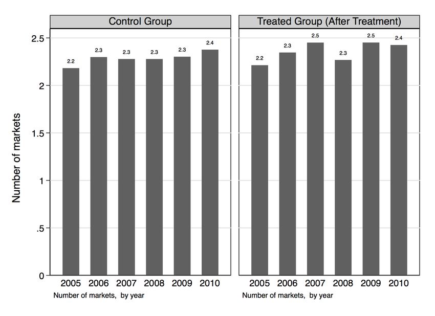
the survey: 2014. We do not have further information on the year of treatment for the perceptions sur-
vey.13 . Second, ITCEQ reported difficulties in following up with some firms, and therefore there is a
slight attrition bias.14 The perceptions survey is therefore only used descriptively and is not the main
basis of the analytical work.

4          Identification strategy and econometric approach

4.1        Identification of treated firms

We faced administrative barriers in matching firm ID numbers to the national business registry data
and reliability issues related to the quality of firm IDs. Therefore, part of the barriers to conducting a
direct matching was administrative, while others were technical. To address these concerns, we took an
approach that most closely resembles an intention-to-treat design that identifies firms that were likely
treated, but among whom compliers are unknown.

To identify firms, we merged firm-level treatment identifiers containing information on firm characteris-
tics such as size, sector, locality, and exporter status. Critically, this information was available for firms
treated each year from 2005 to 2011. Therefore, our analysis is only on firms treated between these
years, with outcomes 1–3 years after treatment. In terms of treatment information, the year of treatment
reflects the first year of treatment, but no information is known about subsequent treatments, nor the
length of treatment.15 While not a perfect approach, this method is associated with a downward attenu-
ation bias of our point estimates. All results reported here, therefore, are lower-bound estimates.

In practice, this is similar to the steps taken in the recent paper by Criscuolo et al. (2019), who also faced
difficulties on direct firm identification by firm ID numbers when evaluating a large-scale firm-subsidy
programme. We can consider the resulting outcome as intention-to-treat effects and a lower bound of
the average treatment effect since there is a percentage of firms in the treatment group that may not
have been treated in reality and some who may have been treated but misplaced into the control group
(Chakravarty et al. 2019). We discuss how we test our identification strategy further in the sensitivity
analysis in Section 5.3.

4.2        Econometric approach

This paper’s econometric approach has multiple steps. As a first step, the paper reports OLS panel fixed
effects outcomes with and without controls. Because there is a selection bias to get treatment from the
IUP, in the casual inference framework a simple OLS will be biased. One method for overcoming this
bias is to find similar control groups that, at least observably, have similar characteristics to those in the
treated group. In practice, the matching literature following the seminal work of Rosenbaum and Rubin
(1983) is a first step in trying to find comparable firms. In the process, we compared matching algorithms

13 This   is different from the source where we identify treated firms, where we do have the year of treatment
14 Theattrition bias is less than 10 per cent in the data, as reported from the ITCEQ report. Unfortunately, it was not possible
to combine this perceptions survey with the RNE due to administrative barriers and authorization requirements.
15 In total, the treatment identifiers contained 128 sectors, ranging from small to large firms with different export activities
totalling 2500 such combinations across the span of years 2005–11. The ‘strata’ of identified treated firms that is a result of
the imperfect identification limitation captures firms that are highly likely to be treated in reality. This strategy is synonymous
with a theoretical intention-to-treat model in which there are compliers and non-compliers. The treated groups are weighed
by the number of treatments and the number of treated firms within the universe of each stratum. For example, if two firms
had the same characteristics and were identified as one treated firm, their group was assigned a weight of 0.5 to account for
potential bias in the identification step. More information on the testing of this identification is presented in Section 5.3.

                                                                5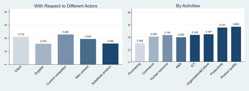
using different calipers and adjustments through bootstrapping, double-robust methods, and a dynamic
panel matching model.16 There were no substantial differences in the estimates, and a marginal change
in standard errors.17 We decided on a distance caliper of 0.001 that reduced the number of firms in our
comparison group, but left enough firms in the regression to allow us to use various time-invariant and
time-variant controls.

Next, we generated the inverse propensity scores within the common support range and included them
in a weighed differences-in-differences regression (IPWDID) as in Hirano et al. (2003), Imbens and
Wooldridge (2009), and Cadot et al. (2015). Imbens and Wooldridge (2009) argue that, asymptotically,
the use of estimated propensities leads to a more efficient estimator as compared to true propensities.
Furthermore, they find that after estimating propensities, the weights given to observations are unbiased.
However, one caveat of this method is that very small and very large propensity scores can lead to
problems. The intuition behind this problem is that weights will be either too heavy or too weak at the
extremes of the distribution and can lead to imprecise estimations. Nevertheless, this issue is less severe
in the IPW estimator than a non-weighted regression because the IPW estimator at least reflects the
uncertainty of the estimation.18 In addition to the standardized IPW process, we also include additional
weighting to address the issue of non-compliers in our identification strategy, as discussed in the previous
section.

Our full econometric specification model is as follows:
                                                           n=3
              yi,t =β0 + β1 Treated ∗ A f teri,t + β2 ∑ Treated ∗ A f teri,t+n + β3 TreatmentGroupi +
                                                           t+n
                                                   n
                                                                                                                            (1)
                     β4 Anticipationi,t−1 + β5    ∑    Treated ∗ A f ter ∗Yeari,t + β6 Xi,t0 γ   + τt + λ i + ζi + εi
                                                   t

where the main variable of interest, yi,t , is firm-level outcome. Depending on the regression, the main
outcome variable will be (the log of) employment, (the log of) average wages per worker, and (the log
of) net job creation.19 A description of all variables is available in Table A1.20 β1 captures the interaction
term of the treatment in the year of treatment. This interaction term is our main variable of interest. β2
is a series of time-specific treatment effects that capture the impact of the programme 1–3 years after
treatment. β3 captures the change of the main outcome variable associated with belonging to the treated
group. This variable is dropped in the fixed effects panel model but retained in the IPW individual fixed
effects model with clustering at the firm level. β4 estimates the anticipation effect of the programme,
one year before treatment. β5 is a year-specific treatment effect that controls for interactions that the
treatment has in each specific year of treatment. β6 captures the impact of a series of control variables,
including age, age-squared, size, distance to ports, and lagged and growth components of the production
function. The lagged and growth components control for non-linear time trends before treatment. They
include the second lags plus averages of the past 2–4 years of the log of employment, average wages,
net job creation, profit, sales, and exports. In the final specifications, we also control for time trends in

16 Double-robust post-estimation regression-adjustment is an additional procedure that corrects bias in the standard errors when

either the propensity score model or the regression model is incorrectly specified.
17
 There were no substantial differences and the analysis with bootstrapping, double-robust estimations, and dynamic panel
models requires more computing power than available in the computers in the INS.
18 More recent proposals for the use of inverse propensity weighting in dynamic treatment models and their applications are
being presented by van den Berg and Vikström (2019).
19 All   estimates are in TND deflated for world prices.
20 While we would have liked to calculate productivity, the database is missing key investment and intermediate input variables.

                                                                 6
the treatment variables with time-treatment fixed effects. Finally, we apply year (τt ), regional (λ i ), and
sector (ζi ) individual fixed effects.21
5 Descriptive analysis and regression results
5.1 The perception survey and descriptive findings from the national firm registry
Only one qualitative evaluation of the IUP has been carried out in recent years. The ITCEQ survey ad-
ministered to IUP recipients collected data on the perceptions of treated and a random set of non-treated
firms with retrospective information from 2014 and 2015.22 The survey found that in the past, treated
firms (treated at any point in time) were underperforming against non-treated firms. In comparison to
non-treated firms, treated firms less often reported increases in revenue, and less often reported increases
in revenue from exports, and employment (Figure 2 and see Figure A2 in the Appendix). If there is no
heterogeneity in financial reporting between firms that were treated and those that were not, this sug-
gests that firms were not selected for treatment based on pre-existing performances. On the other hand,
a higher share of treated firms had expectations of growth in revenues and employment for the next three
years.If this is the case, we should be able observe this empirically.23
However, how do these qualitative descriptive findings compare when we evaluate similar outcome
variables using registered data on firms (RNE)? To gather similar data from the RNE, we need to create
two groups to reflect the groups in the ITCEQ survey, a treatment group (without specifying which
year they were treated), and one that includes a comparable set of firms. Descriptive statistics from
the national firm registry show only level differences between the treated and control groups, but no
difference in growth trends. After treatment, average employment is higher in treated firms, but treated
firms pay lower average wages (Figure 3). Interestingly, average revenue per worker is lower after
treatment for firms in the treated group than in the control group.
21 When this combination over-identifies the desired estimation, we use fewer controls and describe it in the table.
22 The ITCEQ asked firms to report sales, employment, and exports for previous years.
23 In addition to better future revenue and employment expectations, a higher share of treated firms expected to increase
investments after treatment as compared to control firms. The type of investments expected by treated firms differs from
those in the control group (Figure A3). Firms belonging to control groups expected higher material investment, whereas more
treated firms expected to have more immaterial investments. (While it is not possible to decompose total investment by origin
within the ITCEQ survey, the channelling of programme funds to increase immaterial investment suggests that the IUP could
have had a substitution effect rather than a complementary effect on firm investments as we saw in the crowding-out effect
reported by Wallsten (2000). Unfortunately, without further information on capital and investment on a firm level, we cannot
investigate this trend.) Third, treated firms believed that they were more competitive after treatment. They reported having
observed the most improvements in product quality. Treated firms increased productivity, organization and culture, ICT, and
human resources (Figure A4 in the Appendix), as well as used more innovative technology, communications infrastructure,
and automated technologies in the workplace (Figures A5 and A6 in the Appendix). For treated firms, the most considerable
innovations were innovations in the process and the product, to a lesser degree in innovations in firm organization, and to the
lowest degree in marketing. In terms of tangible aspects of innovation, 10 per cent more treated firms reported registering
trademarks and filing patents or licences. Remarkably, there were approximately 30 per cent more treated firms that reported
filing for ISO 9001 certificates—an international standard that measures the quality of products—than firms in control groups.
7Figure 2: Reported increases in employment, revenue, and export outcomes (perceptions survey)
Note: The figure reports the percentage of firms reporting any type of increase of each outcome.
Source: Authors’ calculations based on ITCEQ survey.
Figure 3: Employment, revenue, and wages, 2000–17 (registered data)
Note: To make a comparison with the ITCEQ survey, the figure compares firms that were ever treated after treatment, and
firms that were never treated.
Source: Authors’ calculations based on RNE.
8It is likely that the differences in employment, wages, and revenues between the perceptions survey
and the registered data are due to the Hawthorne effect—differences are purely due to the perception
that outcomes will be better because of treatment.24 While most evaluations of industrial policies are
conducted using perception-based surveys, this comparison shows that perception-based surveys are not
an optimal tool for understanding the impact of such programmes. As with other perceptions-based
surveys and studies, there are strong incentives for reporting managers to provide overly optimistic
responses and be affected by the pure effect of being in the treatment group. The differences between
the perceptions survey and the analysis using registered data illustrates why impact assessments linking
programme treatment with outcomes for firms are essential.
5.2 Regression analysis
Generating propensity scores to adjust regression analysis
The first step of our analysis involves the estimation of propensity scores. We use a simple logit model
to estimate the propensity to be treated. Variables were matched on firm characteristics, including size,
restrictiveness, firm origin (foreign or national), firm type (public or private), year, sector, age, age-
squared, and coastal (regions by the coast).25 Like Cadot et al. (2015), the matching criteria also included
two-year lags and the average of the 2-4 year lags of employment, total wages, profits, and turnover
that accounts for previous trends and avoids direct temporal endogeneity. To control for export ease,
we calculated the average distance to the closest two ports using the territorial distance from the city
centre where the firm was located to the ports.26 A summary table of the sample differences between the
matched treatment and control group is available in Table A2.27 The resulting propensity score measured
the average treatment effects of the intention-to-treat group and dropped observations that did not fit in
the common support range of propensity scores.28
The graphical results of the matching procedure based on several outcomes are presented in Figures 4
and 5. Graphically assessing the matching quality of covariates in treated and control groups suggests
that the distribution of each of the variables is very similar in both groups (Figure 4) and that they both
follow a normal distribution. The bias reduction associated with this process is depicted in Figure 5,
24 Thisis why placebo tests were introduced to perception-based experiments in physical sciences. Alternatively, they may be
due to misreporting in registered data. For misreporting to have a net effect, all treated firms would have to similarly misreport,
such that the outcome shows no systematic difference between the growth rates of the two groups. We believe this is not
credible.
25The coastal variable captured trends associated to being located on the coast of Tunisia rather than inland. Much of the
economic activity lies in the coastal regions.
26 Distance-to-ports variables were estimated using geographical distances from GPS coordinates of the city where firms were
located to the GPS coordinate of all current ports in Tunisia. Using the average of two ports establishes some degree of stability
of access to ports and other markets in case of recent developments in port expansions.
27 Inthe process of estimating the propensity scores, we applied several matching methods starting with the simplest matching
algorithm and extending it to tighter restrictions. Following this, we tested whether the performance of the matching improved
using Rosenbaum tests, and observed the density plots of propensity scores for treated and control groups. Among the meth-
ods used, we applied a strict dynamic Mahalanobis matching, one-to-one nearest-neighbour matching, and kernel-matching
procedures with various sizes of calipers. Observing covariate matching and analysis of Rosenbaum bounds on matching esti-
mators guided the selection of matching procedures. In consideration of the marginal changes and the limited improvements
of matching using more complicated procedures, we pursued a matching algorithm with a caliper of 0.001, restricted to the
common support area, that uses the Abadie and Imbens (2006) standard errors with conditional covariances calculated using
two neighbours. Computational limitations on-site and time access controls limited how many variations of the algorithm we
were able to appropriately assess using our final specifications, but in practice not much changed between different matching
options. The initial matching procedure with different calipers and a full Mahalanobis-metric matching reduced matching bias
in approximately the same amount, but was heavier in computational power.
28 We decided against using a dynamic replacement model both because of computational limitations and because we want to
prioritize consistently estimating the closest matching propensities within the regressions.
9which consists of a list of all matching covariates, and graphically illustrates the gains in comparability
resulting from the removal of observations outside the common support and further away from the
propensity values of the treated variables.
Figure 4: Matching performance: kernel density of employment and wages
Source: Authors’ calculations based on RNE.
Figure 5: Matching performance: variable bias reduction
Source: Authors’ calculations based on RNE.
After the removal of firms outside the common support, there were approximately 2,000 treated ob-
servations, and approximately 68,000 observations in the control group. These numbers were similar
when we ran matching algorithms separately for employment and wages. While the matching perfor-
mance looks promising, there are still caveats. We argue, however, that regression adjustment methods
such as the IPW builds on a simple OLS. The limitations to the use of the propensity score method are
well-known (Caliendo and Kopeinig 2008; Dehejia and Wahba 2002; King and Nielsen 2019).
In the literature, there are, in general, two types of issues that occur when using propensity scores in
estimation procedures. The first involves how the researcher uses the method, and the second involves
its econometric limitations. To avoid the first type of issue, we started from the most stringent model,
based on the empirical literature that uses this method. One-by-one, we relaxed conditions until we
found a combination that brought us the closest to finding matched pairs using both visual propensity
score plots and bias reduction summary statistics after matching. We pursued the model on which we
were able to include a reasonable amount of controls in the final IPW regression without losing so many
observations that our regressions with standard controls were over-fitted.
10The second issue is addressed in how we defined our matching algorithm and used it in the next step.
We matched on pre-trends and reintroduced controls in the regression adjusted model that incorporated
propensity scores. We controlled for lagged trends, current individual fixed effects, and average time
trends. The variable that caused the most difficulty was matching on lagged 2–4 years. While this in-
creased the credibility of our matching process, it also limited the availability of years for our regression,
as each observation would now need at least four prior years of data and three years of data after the year
of treatment. This automatically limited our analysis to firms that had at least seven years of continuous
information.
The use of the propensity score matching method is only an initial step in our analysis. The propensity
scores are then integrated as weights into our differences-in-differences analysis, which theoretically
reduces our bias and improves our estimations from our original OLS differences-in-differences model
(Imbens and Wooldridge 2009). While ignorability of matched assignments given observable character-
istics may still be a concern, our matching outcomes are not the final results of our estimation strategy.
With the IPWDID we have the opportunity to apply additional control variables in a second stage that
attempts to control for selection on observed growth and time-trend variables.
Regression results on wages
Results for the impact of the programme on wages and employment are reported in Tables 1 (wages)
and 3 (employment). We report the basic OLS results of treatment with and without controls in columns
(1)–(3). In column (1) of Table 1 with only year and sector controls, we see that there is no statistically
significant impact of this programme on wages. However, there is a positive anticipation effect the year
before treatment. Wages increase by 3 per cent the year before treatment. This is consistent with a story
that suggests that firms may anticipate demand for higher-waged workers, or rearrange the occupation
composition of workers towards workers in higher-paid occupations. We then add further controls for
size groups of firms, the age of firms (age and age-squared), the origin of the firm (foreign or local), the
type of firm (public or private), whether the firm is geographically in the coastal regions, whether the
firm is only an exporting firm (or also sells locally), the distance to the nearest port, and various controls
for growth.29 . Column (2) reports estimates after the inclusion of these additional control variables. The
estimated effect of the programme on wages is still not statistically different than 0. However, there is
growth in wages in the three years following treatment that is consistently close to 2 per cent. When
including additional controls, the anticipation effect is reduced by one-third of its original estimate.
Lastly, in column (3), if we include controls for the year-specific treatment effect,30 the impact of the
programme on wages is positive, although small, but significant at the 5 per cent level in the year of
treatment, and the three years following treatment. A treated firm has, on average, 1.3 per cent higher
average wages, and the impact doubles to close to 2 per cent in the following years.
29 This includes growth of employment, wages, net job growth, sales, and export value from the previous year; the lag of the
values of the same variables, and the 2–4 year lag of values of those same variables.
30 This is an interaction between when the firm is treated and the fact that it is treated in a specific year.
Its purpose is to control
for time-specific treatment effects that may vary from year to year. This includes individual controls for treatment in 2000,
2001, and so on.
11Table 1: Impact of the IUP on average wages, 2000–17
Log of OLS fixed effects models Reg. adj. models
ave. wages (1) (2) (3) (4) (5)
PSM IPW
Treatment –0.003 0.007 0.013** –0.070*** 0.023**
[–0.447] [1.208] [2.081] [–5.134] [2.249]
One year after 0.004 0.018*** 0.021*** –0.006
[0.579] [3.621] [3.646] [–0.486]
Two years after 0.007 0.020*** 0.020*** –0.012
[1.118] [3.625] [3.249] [–1.133]
Three years after 0.003 0.019*** 0.017*** –0.008
[0.430] [3.126] [2.605] [–0.672]
Anticipation 0.030*** 0.011** 0.022*** –0.008
[4.654] [2.052] [3.687] [–0.637]
Treat * year No No Yes No Yes
Age controls No Yes Yes Yes Yes
Growth and lags No Yes Yes Yes Yes
Type and origin No Yes Yes Yes Yes
Coastal and port No Yes Yes Yes Yes
Year and sector Yes Yes Yes Yes Yes
Observations 327,234 195,501 195,501 69,077 69,077
R-squared 0.347 0.458 0.458 0.0004 0.693
Method FE FE FE PSM IPW
Note: Robust t-statistics in brackets. *** p < 0.01, ** p < 0.05, * p < 0.1. IPW estimates are double weighted. The first weight
corresponds with a logit propensity that weights control and treated groups by their propensity to be treated. The second
weight is a correction weight from the identification strategy. The number of firms in the OLS model is 34,559 for column (1)
and 28,336 for columns (2) and (3). The differences between the models are due to a lack of historical information for 2–4
years prior to when the firms appear in the database.
Source: Authors’ compilation based on RNE.
Nevertheless, selection bias due to the firm application procedure, the selection procedure, and the type
of treatment they received would imply that treatment and control groups are not comparable. To get a
more credible estimate, it would be best to compare similar groups that at least have similar observable
characteristics. As previously discussed, our method to address this issue is to estimate the probability
of treatment in the year t (propensity score) and integrate this into an inverse weighted differences-in-
differences model. Column (4) of Table 1 provides an estimate of the average treatment effect when
matching on observable covariates, without the interacted year and treatment effects.31 The estimation
of the average treatment effect is counter-intuitively –7 per cent. However, the estimation’s power is very
low (R-squared is 0.0004). When we use the propensity score from this logistical regression and include
time-specific treatment effects, our estimated impact of the programme on wages is +2.3 per cent in the
year of treatment and not significantly different from 0 in the years thereafter. The explanatory power of
this IPW model in column (5) suggests that there is less variance in the error terms in this specification.
The difference between the OLS and the IPW model suggests that a simple OLS was indeed suffering
from selection bias. If this was not the case, we would have expected the OLS results to look similar to
the IPW results that measure differences between observationally similar firms.
Not all firms experienced the impact of the IUP in the same way (Table 2). The most substantial pos-
itive impact on wages—in order of strength in magnitude—is in small firms (5–9 employees), small
to medium firms (10–19), and medium firms (20–49). Small firms increased wages by close to 18 per
cent one year after treatment. Wages in firms with 10–19 employees were more volatile but were net
positive 2–3 years after treatment. Lastly, medium-sized firms with 20–49 employees showed a 9 per
31 With these included, the logistical regression to estimate the propensity for treatment was over-identified.
12cent increase in wages in the year of treatment. This increase was followed by a 5 per cent and a 4.5 per
cent growth in average wages 2–3 years after treatment.
Table 2: Impact of the IUP on average wages, by size
Log of wages (1) (2) (3) (4) (5) (6)
Small Sm-Med Medium Med-Lge Large Very lge
[5, 9] [10, 19] [20, 49] [50, 99] [100, 199] [200, 999]
Treatment –0.004 0.015 0.091*** 0.049*** 0.019 0.059***
[–0.082] [0.528] [4.594] [3.256] [0.918] [3.985]
One year after 0.177*** –0.0003 0.050* –0.021 –0.063*** –0.019
[4.735] [–0.009] [1.759] [–1.319] [–3.048] [–1.065]
Two years after 0.219 –0.090** 0.030 –0.031* –0.048** –0.031
[0.861] [–2.294] [1.240] [–1.944] [–2.353] [–1.568]
Three years after –0.134 0.119** 0.045** –0.015 –0.036 –0.009
[–1.578] [2.116] [2.047] [–0.900] [–1.503] [–0.504]
Anticipation –0.024 –0.043 –0.002 –0.066*** –0.005 –0.030
[–0.302] [–1.333] [–0.085] [–4.196] [–0.190] [–1.566]
Observations 31,203 12,108 11,314 6,496 4,344 3,354
R-squared 0.783 0.771 0.768 0.745 0.647 0.795
Method IPW IPW IPW IPW IPW IPW
Note: Robust t-statistics are in brackets. *** p < 0.01, ** p < 0.05, * p < 0.1. Controls includes fixed treatment group effect,
year, treatment and year interaction effects, sector controls, growth and lags of only wage variables. Because of a more limited
number of observations, we could not include other controls. The method is IPW with standard errors clustered at the firm level.
Source: Authors’ compilation based on RNE.
There was some impact on medium to large (50–99), large (100–199), and very large firms (200–999),
but the results do not suggest that the changes due to the IUP were as strongly in favour of higher wages
as they were in small firms. Wages grew in the first year for medium to large firms (50–99) and very
large firms (200–999), but the growth in wages was to a lesser degree than the growth observed for
smaller firms. Furthermore, wages in these two types of firms dropped again 2–3 years later. Medium
to large firms may have had positive increases in wages the year of treatment, but the increases were
anticipated with a drop in wages the year prior to treatment. These estimates suggests that, in the year
prior to receiving treatment, firms either dismissed high-wage workers without replacement or that low-
wage workers replaced high-wage workers. Therefore, the growth in wages in the first year of treatment
may have either been firms re-hiring high-wage workers or temporarily augmenting salaries. But this
growth does not last and even shows signs on a net decrease two years later. Lastly, large firms with
100–199 employees showed a decrease in average wages 2–3 years after having received treatment from
the IUP. For large firms, average wages dropped by 6.3 per cent in the second year after treatment, and
4.8 per cent in the third year after treatment. As we will see in the employment section in Table 4, this
drop in wages was accompanied by a 3 per cent growth in employment in the third year. Jointly, this
suggests that the programme was not effective for jobs creation and quality in large firms, but it is likely
that the employment strategy in large firms changed after IUP treatment to one with more low-wage
labour.
Regression results on employment
On the aggregate level, we observe a sizeable impact on employment in the first year of treatment
and every year thereafter when we only control for year and sector fixed effects (column (1) in Table
3). There is also a relatively large and strong anticipation effect one year before treatment. However,
including additional controls diminishes the impact of the programme sharply (down to 1–2 per cent)
and the anticipation effect becomes statistically insignificant (column (2) in Table 3). These estimates
suggest that most of the initially observed growth in employment is explained by the characteristics of
the firms rather than the treatment.
13Table 3: Impact of the IUP on employment
Log of OLS fixed effects models Reg. adj. models
employment (1) (2) (3) (4) (5)
PSM IPW
Treatment 0.260*** 0.016*** 0.011* 1.545*** 0.001
[19.282] [2.745] [1.658] [52.40] [0.162]
One year after 0.133*** 0.021*** 0.015** 0.005
[10.221] [3.804] [2.411] [0.612]
Two years after 0.093*** 0.020*** 0.017*** 0.001
[6.996] [3.507] [2.792] [0.115]
Three years after 0.099*** 0.013* 0.014** 0.012
[6.177] [1.940] [2.010] [1.166]
Anticipation 0.169*** 0.009 0.003 –0.016
[12.415] [1.570] [0.433] [–1.549]
Treat * year No No Yes No Yes
Age controls No Yes Yes Yes Yes
Growth and lags No Yes Yes Yes Yes
Type and origin No Yes Yes Yes Yes
Coastal and port No Yes Yes Yes Yes
Year and sector Yes Yes Yes Yes Yes
Observations 328,536 195,501 195,501 69,077 69,077
R-squared 0.010 0.606 0.606 0.038 0.949
Method FE FE FE PSM IPW
Note: t-statistics are in brackets. *** p < 0.01, ** p < 0.05, * p < 0.1. IPW estimates are double weighted. The first weight
corresponds with a logit propensity that weights control and treated groups by their propensity to be treated. The second
weight is a correction weight from the identification strategy. The number of firms in the OLS model is 34,234 for column (1)
and 28,336 for columns (2) and (3). The differences between the models are due to a lack of historical information for 2–4
years prior to when the firms appear in the database.
Source: Authors’ compilation based on RNE.
Table 4: Impact of the IUP on employment, by size
Log of employment (1) (2) (3) (4) (5) (6)
Small Sm-Med Medium Med-Lge Large Very lge
[5, 9] [10, 19] [20, 49] [50, 99] [100, 199] [200, 999]
Treatment 0.518*** –0.031 0.010 –0.005 0.019* –0.082***
[12.203] [–1.577] [0.689] [–0.502] [1.712] [–3.981]
One year after 0.135 0.076* 0.047** 0.033** –0.013 –0.047**
[1.465] [1.910] [2.225] [2.481] [–1.064] [–2.298]
Two years after 0.127* 0.110** 0.012 0.012 0.014 0.003
[1.719] [2.530] [0.456] [0.868] [1.037] [0.116]
Three years after –0.095 –0.064 0.097*** 0.002 0.037** –0.023
[–0.846] [–1.620] [3.506] [0.098] [2.426] [–0.794]
Anticipation 0.173*** 0.013 0.023 –0.025** 0.014 –0.074***
[3.039] [0.398] [1.108] [–2.008] [0.936] [–3.013]
Observations 31,203 12,108 11,314 6,496 4,344 3,354
R-squared 0.269 0.103 0.149 0.135 0.131 0.362
Method IPW IPW IPW IPW IPW IPW
Note: Robust t-statistics are in brackets. *** p < 0.01, ** p < 0.05, * p < 0.1. Controls includes fixed treatment group effect,
year, treatment and year interaction effects, sector controls, and growth and lags of only employment variables. Because of a
more limited number of observations, we could not include other controls. The method is IPW with standard errors clustered at
the firm level.
Source: Authors’ compilation based on RNE.
As in the previous regression analysis, there are still significant differences between the treatment and
control groups that are due to selection bias, making a direct comparison between the two groups im-
possible. To address this, we integrated propensity scores in regressions, adjusted to include propensity
weights. The average treatment effect from the simple matching exercise in column (4) of Table 3
14shows that employment increased substantially, as do the OLS models with fixed effects in columns
(1–3). However, the treatment explained very little of why employment increased (R-squared of 0.038,
as compared to 0.606 in the OLS panel fixed effects model). When we integrate the probability of be-
ing in the treated group in our differences-in-differences model, our estimates are no longer significant.
The inverted propensity score difference-in-differences regression has a rather high explanatory power,
with an R-squared of close to 1. The explanatory strength of this specification suggests that changes in
employment were not likely due to the IUP treatment.
Nevertheless, these results were not homogeneous for all firms. In the year of treatment, small firms
(5–9 employees) grew by close to 50 per cent and continued to grow two years after treatment. They
increased employment the year before treatment. Small to medium-sized firms (10–19) grew in the first
and second years after treatment. Medium-sized firms (20–49) grew in the first and third years after
treatment. At least in small firms, firms increased employment in anticipation of treatment.
There was some measurable impact on employment in firms with over 50 employees, but positive im-
pacts were smaller in magnitude, and in some cases the impact was negative. For example, in medium
to large firms (50–99) there was a 3 per cent growth in employment the year after treatment, but this
growth was smaller than other groups and was preceded by a similarly sized decrease in employment in
anticipation of the treatment. Large firms (100–199) saw a 3.7 per cent increase in employment the third
year after treatment, but this coincided with two previous years of drops in wages (from Table 2). Most
strikingly, the programme was the least supportive of labour in very large firms (200–999). In very large
firms, the programme had a negative impact on employment (8 per cent) in the year of treatment and
a 4.7 per cent decrease in the first year after treatment. For these firms, the large drop in employment
coincided with the year of a large drop in wages. This fall in employment and wages suggests that large
firms adopted strategies not very beneficial for labour (such as restructuring).
Trends in net job creation32 provide additional support for the findings on employment by looking at the
churning patterns of firms within each size group (Table 5). Our decision to include this is to address
the concern that stronger growth in smaller firms could only be due to composition effects. In columns
(1)–(3), firms in the small to medium-sized groups all show an increase in net job creation in the year of
treatment, even if there were some anticipation effects in the small to medium and medium categories.
There are almost no measurable results of the programme on net job creation in larger firms. While
medium to large firms (50–99) may have some growth in net job creation, it is in the third year, and
smaller than the growth in the smaller firms. There is a negative (but not very significant) impact of the
program on net job creation in very large firms (200–999).
Size and industrial policies
On an aggregate level, the IUP marginally improved wages (2.3 per cent in the year of treatment column
(5) of Table 1), but there is less convincing evidence that the IUP was good for employment. Taken at
face value, the global picture shows that the programme increased wages for workers, but did not change
the number of workers employed. This finding is in line with the overarching goals of the IUP.
The heterogeneous estimates of the IUP on wages and employment depict a different story. These re-
sults suggest that the IUP was successful both in terms of employment and wages in smaller firms in the
Tunisian economy. If the strategy of a firm is to increase competitiveness through more qualified work-
ers, then we should observe an increase in wages per worker. If more qualified workers do not crowd
out other types of workers, then we should also see a growth in net job creation, and to a lesser degree
in employment. In smaller firms, we observe both an increase in wages and a growth in employment
32As a reminder, net job creation is an increase in the number of individuals employed, minus the losses in the number of
individuals employed.
15You can also read