Investors and Housing Affordability. y - Carlos Garrigaz, Pedro Getex, Athena Tsouderou December 2019 - American Economic ...
←
→
Page content transcription
If your browser does not render page correctly, please read the page content below
y
                Investors and Housing A¤ordability.

                   Carlos Garrigaz, Pedro Getex, Athena Tsouderou{

                                        December 2019

                                             Abstract

         This paper studies the impact of housing investors on the dynamics of housing a¤ord-
     ability, after the Global Financial Crisis. Using an instrumental variable approach, we
     …nd that the investors’ purchases in the U.S. MSAs, increase the price-to-income ratio,
     especially in the bottom price-tier of the market, and in areas with large supply restric-
     tions. However, these e¤ects are short-lived. Investors cause a signi…cant supply response,
     as they increase granting of new building permits. In the medium-term, investors’ pur-
     chases lead to reductions in prices and improved a¤ordability. These …ndings should be
     considered when designing policy regulations.

         Keywords: Investors, Housing Prices, A¤ordability, Homeownership, Real Estate
     Investment.

     We thank Itzhak Ben-David, Henning Bohn, Daniel Cooper, Stefano Corradin, Morris Davis,
Ignacio De la Torre, Anthony DeFusco, David Echeverry, Michael Ehrmann, Daniel Fernández Kranz,
Andra Ghent, Juan-Pedro Gomez, Pere Gomis-Porqueras, Deeksha Gupta, Jonathan Halket, Lu Han,
Marie Hoerova, Ivan Jaccard, Dirk Jenter, Nina Karnaukh, Daniel Kelly, Finn Kydland, Agnese
Leonello, Jose Maria Liberti, David Ling, Haoyang Liu, David Marques, Clara Martinez-Toledano,
Brian Melzer, Erwan Morellec, Charles Nathanson, Alex Popov, Michael Pries, Lev Ratnovski, Michael
Reher, Rafael Repullo, Stephen L. Ross, Gerhard Runstler, Vahid Saadi, Glenn Schepens, Martin
Schneider, Jean-David Sigaux, Jirka Slacalek, Alejandro Van der Ghote, Randal Verbrugge, Je¤rey
Zabel, Fernando Zapatero, and seminar participants at Durham, ECB, NEOMA, Notre Dame, IE,
Ohio State, and 2018 UEA, 2019 HULM, 2019 AREUEA International, 2019 AEFIN Finance Forum,
and 2019 SED Conferences.
   y
     The views expressed herein do not necessarily re‡ect those of the Federal Reserve Bank of St.
Louis or the Federal Reserve System. The results and opinions are those of the authors and do
not re‡ect the position of Zillow Group. Research reported in this paper was partially funded by
the Spanish Ministry of Economy and Competitiveness (MCIU), State Research Agency (AEI) and
European Regional Development Fund (ERDF) Grant No. PGC2018-101745-A-I00.
   z
     Federal Reserve Bank of St. Louis. carlos.garriga@stls.frb.org.
   x
     IE Business School, IE University. pedro.gete@ie.edu.
   {
     IE Business School, IE University. athena.tsouderou@student.ie.edu.

                                                 1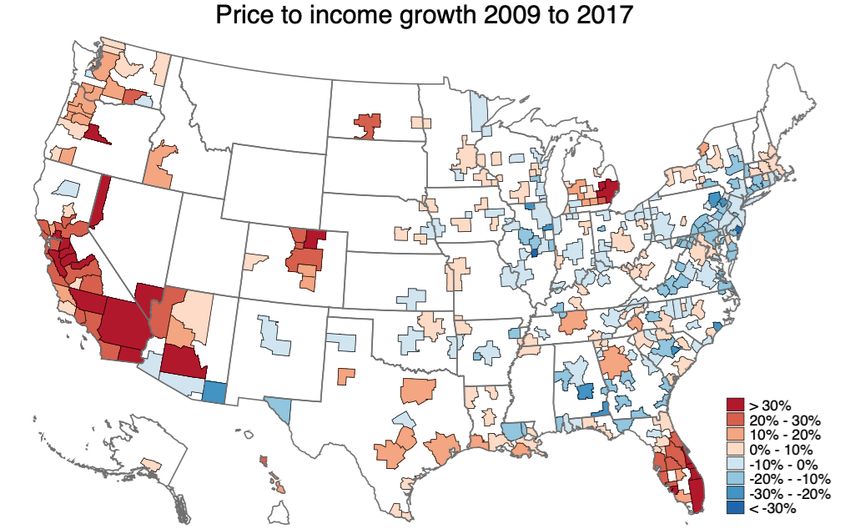
Introduction
Housing a¤ordability is one of the most critical policy challenges for most cities in the
world (Favilukis, Mabille and Van Nieuwerburgh 2019). For example, in 2019, in more than
55% of the U.S. MSAs the median household needs at least three times their annual income
to buy a median-priced home. Figure 1 shows that this level of a¤ordability resembles the
situation during the large housing boom of the 2000s.
Interestingly, it has become common to link a¤ordability problems to the explosive growth
of institutional investors in housing markets (see for example ACCE Institute 2018; the Wall
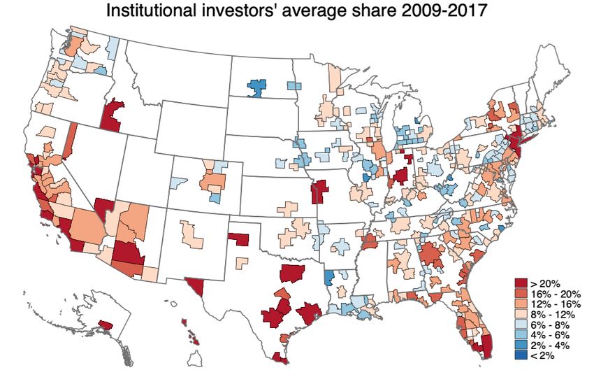
Street Journal 2017; or the Guardian 2019). These concerns are supported by …gures, as Figure
2, which shows that the MSAs that experienced the highest increase in the price-to-income
ratio also had a corresponding contemporaneous increase in the market share of institutional
investors. O¢ cials in several cities have enacted or are discussing policies to block investors.
For example, New York and California, where presence of institutional investors has reached
unprecedented highs, recently approved statewide rent controls (Business Insider 2019). Am-
sterdam wants to directly ban investors from buying and renting properties. Spain recently
imposed a set of measures to penalize them. Berlin is considering to expropriate large, private,
pro…t-seeking landlords (The Wall Street Journal 2019).
This paper contributes to the debate, whether housing investment is good or bad for a¤ord-
ability. Using a rich database covering the whole U.S. from 2009 to 2017, we quantify the e¤ects
of institutional investors in housing markets post-…nancial crisis. We exploit variation across
MSAs in the presence of institutional investors, and perform various analyses, …rstly in the
cross-section and secondly dynamic using panel data.1 Our results show causal evidence that
the presence of institutional investors has been a signi…cant driver of the housing price recovery
since the …nancial crisis. However, our paper also shows an equilibrium response of supply:
investors increase the supply of housing and eventually reverse the price growth. Investors
eventually contribute to making houses more a¤ordable to purchase.
Our identi…cation strategy exploits heterogeneity across the U.S. MSAs in the market share
of housing purchases by institutional investors. The challenge for our identi…cation is to isolate
shocks to investment in the housing market from shocks that drive both housing variables
and the share of housing purchases by institutional investors. For example, an ordinary least
squares (OLS) regression of price growth on investors’market share would be biased downwards
1
We de…ne institutional investors as legal entities who purchase homes, that is, they purchase under the
name of an LLC, LP, Trust, REIT, etc.
2
if investors were attracted to areas where prices collapsed during the crisis.2

    We use an instrumental variable approach to overcome the previous challenge. Beginning
in December 2008, the Fed’s Quantitative Easing (QE) reduced the supply of safe assets in the
market. The federal funds rate and the returns on certi…cates of deposits and other safe assets
fell close to zero. In such a scenario, investors who would traditionally invest in safe assets
switch their money to riskier assets. Large amounts are invested in housing. In particular,
knowledgeable investors searching for a stable yield, are more likely to consider buying prop-
erties and renting them out, which would give them a stable rental yield. Consistent with this
“search-for-yield” theory, Daniel, Garlappi and Xiao (2018) …nd that a low-interest-rate mon-
etary policy increases investors’ demand for high-dividend stocks, which is more pronounced
among investors who fund consumption using dividend income. As rents are mostly stable,
housing becomes an investment asset and a close substitute to safe yield-earning investments.

    The QE produced a national shock to the risk-free rates. Our instrument exploits hetero-
geneity across MSAs in exposure to this shock, by measuring the MSAs’exposure to “invest-
ment attitude”, in other words, high-earning, sophisticated, risk-seeking residents. The idea is
to identify whether a particular MSA has a large share business income earned by the MSA
residents, as a proxy for a large propensity to invest and or understand investments. Facing
more attractive terms for investment in housing after 2008, investment-prone high-earning in-
dividuals are likely to direct more capital to the housing market, through new or existing legal
entities. Our analysis of the institutional investors’investment strategy is in line with the view
that investors were searching for yield.

    Our instrument is the average share of value of business income over total income of high
earners in 2007 in each MSA, calculated using tax returns from the IRS. We show that MSAs
with greater exposure to business income of high earners experienced larger share of housing
purchases by institutional investors after 2008. To create the panel version of this instrument we
multiply the 2007 business income share by the certi…cate of deposits rate growth, which we use
to quantify the e¤ects of QE. Since the business income share of each MSA is determined prior
to the QE, there is minimal risk of reverse causality. That is, it is unlikely that housing price
growth during 2009-2017 a¤ected the share of business income in 2007. Our key identi…cation
assumption is that, once we control for an array of factors and …xed e¤ects, exposure to business
income in 2007 is uncorrelated with other drivers of housing markets over 2009-2017.

    We rigorously assess the validity of the instrumental variable. First, we control thoroughly
for an array of local activity shocks, trends during the previous housing boom and bust, and local
  2
   The national housing price index shows that average prices in the U.S. were falling from 2007 to
2012.

                                                3
factors, making it unlikely that the error term re‡ects common movers of both investors and
housing market variables. Second, we provide extensive evidence that in the pre-QE period the
instrument does not correlate with either higher price growth, rent growth, new construction, or
with other factors that drive the housing markets. For example, before 2008 patterns between
MSAs with the highest and lowest exposure to the share of business income are parallel. Third,
placebo tests con…rm that the instrument only captures post-crisis shocks to investment in the
housing markets. Fourth, an alternative instrument from Gete and Reher (2018) that operates
through credit constraints to households, gives us similar results.

    In the cross-section, we …nd that institutional investors signi…cantly increase housing prices
and price-to-income ratios over the 2009-2017 period. One standard deviation larger share
of investors that the mean, increases price growth by eighty to ninety percent of the cross-
sectional standard deviation. It also increases the price-to-income ratio by up to two standard
deviations. The largest e¤ects happen on the bottom price-tier of the market relative to the
top-tier. During this period, the investors increase the supply of housing through a rise in new
construction. The investors also bring more liquidity to the housing market, by reducing the
share of houses that stay vacant.

    To study the dynamic e¤ects of investors, we estimate the response of housing prices and
quantities to the institutional investors’purchases over time, by employing the methodology of
Jordà (2005). This allows for separation of the dynamic adjustment in markets where the short-
run supply elasticity is relatively inelastic. The results indicate that on impact the investors’
purchases have a positive e¤ect on house price growth lasting two years. Between the second
and third year the impact on the growth rate becomes zero, and negative thereafter. The hump-
shaped response of construction, combined with the relatively inelastic short-run housing supply
rationalizes the observed patterns. As investors trigger new construction, the supply of housing
increases and houses become cheaper and more a¤ordable in the areas where investors hold
a larger share of the market. Consistent with our theory, the ‡uctuations in prices are much
larger in areas with low price elasticity of supply.

    This paper contributes to the literature on housing a¤ordability. Housing a¤ordability is
one of the most critical policy issues for most large cities in the world, and more research is
required to inform policy (Deng, Qin and Wu 2019). In their in‡uential paper, Gyourko, Mayer
and Todd (2013) suggest that the inelastic supply of land along with an increasing number of
high-income households at the national level in the U.S., leads to persistent high house prices
in large MSAs and crowds out lower-income households. The e¤ectiveness of various policies
aimed at improving housing a¤ordability is at the core of the recent literature. For example,
Favilukis, Mabille and Van Nieuwerburgh (2019) study the welfare gains of di¤erent key policy

                                                4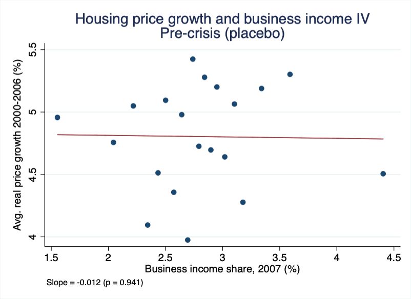
levers. Relative to this literature, our paper explores and provides evidence for a pro-market
approach. By letting markets come to an equilibrium, the response of supply may restore the
a¤ordability levels in the medium-term.

    Our paper also contributes to a new literature that focuses on the emergence of institutional
investors in housing markets after the global …nancial crisis. Garriga, Gete and Tsouderou
(2019), analyzing residential deeds in all U.S. MSAs, show that post-crisis institutional investors
replaced the individual speculators that ‡ooded the U.S. housing market during the previous
housing boom. The authors show that the new institutional investors are mainly small and
local, and their investment strategy is driven by search for yields. In a thorough analysis
of institutional investors, using deeds data from a di¤erent source, Lambie-Hanson, Li and
Slonkosky (2019) …nd that single-family institutional buyers contributed to an increase in price
and rent growth. Their identi…cation is based on the First Look program, a program that gave
households and non-pro…ts an opportunity to bid on real estate owned properties before they
became available to investors.3 Verbrugge and Gallin (2019) …nd that multi-unit landlords,
when renegotiating rent contracts, set rent increases that exceed the in‡ation rate, aided by the
law of large numbers and exploiting tenant moving costs. Graham (2019) …nds that during the
latest housing bust investors substitute for falling homeowner demand, and thereby dampen
declines in housing prices.4

    The rest of the papers in this literature have focused on single-family housing in speci…c
areas in the U.S. For example, Gay (2015) documents that purchases and sales of single-family
houses by institutional investors were four times more in the years 2012 and 2013 compared
to 2011. He …nds that institutional investors buy more properties in lower income areas of
the Chicago Metro Area and sell them at a premium after renovations, which is related to low
a¤ordability of buying a house in those areas. Brunson (2019) …nds that institutional investors
paid a discount of about 8% to 11% per transaction in the Charlotte region post-crisis. Allen,
Rutherford, Rutherford and Yavas (2017) focusing on the Miami-Dade County in Florida, …nd
that an increase in the share of houses purchased by investors in a census block is related to an
increase in house prices. Raymond et al. (2018) …nd that large institutional owners of single-
family rentals …le more frequently eviction notices compared to small landlords in Fulton County
in Atlanta. Mills, Molloy and Zarutskie (2019) show that prices increased in neighborhoods
where large buy-to-rent investors are concentrated. The previous papers however do not use
causal identi…cation.
  3
    The …ndings are also included in a nontechnical report (Lambie-Hanson, Li and Slonkosky (2018)).
  4
    A more established literature has studied foreign and out-of-town investment in the housing mar-
kets. See for example recent papers by Cvijanovic and Spaenjers (2018), Davids and Georg (2019),
and Favilukis and Van Nieuwerburgh (2018).

                                                 5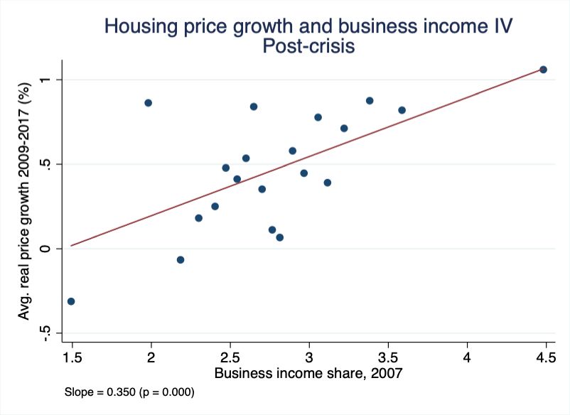
Relative to the previous literature, our paper provides novel insights into the dynamic
e¤ects of institutional investment in housing markets. To the best of our knowledge this paper
is the …rst to study the housing a¤ordability dynamics in response to institutional investors,
and the equilibrium response of supply. Moreover, by introducing and thoroughly defending a
novel instrumental variable based on local “investment attitude” in all U.S. MSAs, our paper
quanti…es the contribution of investors to real e¤ects in the housing markets, and di¤erential
e¤ects for the di¤erent market segments.

    The rest of the paper is organized as follows: Section 1 describes our data. Section 2 presents
our cross-sectional analysis. Section 3 presents our dynamic analysis. Section 4 rigorously as-
sesses the validity of our instrument. Section 5 concludes. The Appendix has extra information
about the variables and more robustness tests.

1     Data

     Data on investors in the U.S. housing market come from the Zillow Transaction and As-
sessment Dataset (ZTRAX), a new database provided by Zillow (2017). The database covers all
property ownership transfers in the U.S., as recorded by the counties’deeds. We focus on own-
ership transfers of residential properties, including multi-family and single-family, in the period
from January 1st, 2000 to December 31st, 2017. Our …nal sample, from which we construct the
investors’purchases variable, consists of 85 million transactions nationally.

    We use a rigorous methodology to identify investors. First we distinguish between individual
and non-individual buyers based on the buyer name. Second, we …lter out buyers that are relo-
cation companies, non pro…t organizations, construction companies and national and regional
authorities, as well as banks, Ginnie Mae, Fannie Mae, Freddie Mac and other mortgage loan
companies and credit unions, and the state taking ownership of foreclosed properties.

    We use the dollar value of purchases by investors instead of the number of purchases to cal-
culate the investors’market share, since the number of purchases would underestimate presence
in the apartments market. For example the number of purchases would equate a purchase of one
condominium to the purchase of one apartment building of 100 apartments. The dollar value of
purchases re‡ects more accurately the presence of individuals and institutional investors in the
single-family and multi-family markets. Our variable of investors’presence is the share of the
dollar value of purchases by investors over the dollar value of all purchases, that is, by investors
and households. The total local market value accounts for economic shocks in each location
that a¤ect residential purchases.

                                                 6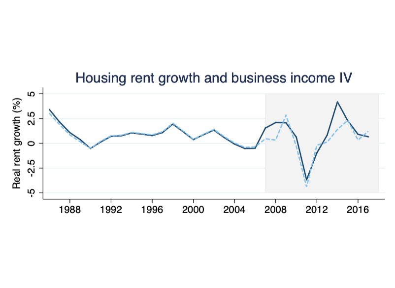
In our robustness checks we use alternative measures of the presence’ of investors based
on the number of properties or the number of units purchased. For example a purchase of a
10-unit apartment building counts as 10 units. The number of units is coded by Zillow. The
online appendix A describes our coding of this variable when there are missing or incomplete
data in ZTRAX.

    The main data source to construct our instrument is the Internal Revenue Services (IRS), in
particular, the Statistics of Income (SOI). This dataset provides zip code data on administrative
records of individual tax returns. Our instrument approximates the average individual’s tax
returns by the zip code returns of a speci…c income group. Since the dataset does not provide
returns at the individual level, the zip code income group level is the closest approximation to
the average individual of each group within the zip code. We speci…cally focus on the returns
of the top earnings groups, which include people with annual adjusted gross income above
$100,000, and we perform robustness for this cut-o¤. Our instrument is the average share of
business income over total income of high earners, in each MSA in 2007. We weight by the
total income of high-earners to aggregate to MSA level. To construct the panel version of the
instrument, we retrieve the average one-year certi…cate of deposits (CD) rate from Bankrate, a
consumer …nancial services company.

    The housing variables come from Zillow. Housing prices come from the Zillow Home Value
Index, a dollar-denominated, smoothed, seasonally adjusted measure of the median estimated
home value across a given region and housing type. This index is constructed using estimated
monthly sale prices not just for the homes that sold, but for all homes even if they didn’t sell
in that time period, which addresses the bias created by the changing group of properties that
sell in di¤erent periods of time.

    Speci…cally, we use the Zillow Home Value Index for all homes, single-family homes, top-
tier homes and bottom-tier homes at the MSA level. The bottom-tier segment of the market
is the bottom third of the housing price distribution in each MSA. The bottom-tier price is
the median price of the segment, that is, the bottom 17th percentile of the prices of the total
market within an MSA. In a symmetrical way, the top-tier segment of the market is the top
third of the price distribution in each MSA, and the top-tier price is the top 83rd percentile of
prices within an MSA. Housing rents come from the Zillow Rent Index for all homes, which is
constructed using a similar methodology to the Zillow Home Value Index.

    To calculate the price-to-income (rent-to-income) ratio, we divide the median housing price
(annual rent) by the median household income from Zillow in each MSA-year. To calculate the
price-to-income ratio for di¤erent market segments, we use instead the individual adjusted gross

                                               7
income from the SOI. The bottom-tier price-to-income ratio is the ratio of the 17th percentile
of housing prices from Zillow over the 17th percentile of individual adjusted gross income from
the SOI. The median price-to-income ratio is the ratio of the median housing price over the
median individual adjusted gross income. The top-tier price-to-income ratio is the ratio of the
83rd percentile of housing prices over the 83rd percentile of individual adjusted gross income.

   We collect the number of new construction permits from the Census Bureau’s annual Build-
ing Permits Survey. The permits distinguish among single-family, two-family, three- or four-
family, and …ve-or-more family buildings. Finally, we collect MSA-year level controls, which are
population from the U.S. Census Bureau, unemployment rate from the U.S. Bureau of Labor
Statistics, and median household income from Zillow.

   A more detailed description of the data sources is included in the online appendix A. To
summarize, there are 332 MSAs with the full set of average housing variables and investors’
market share for the years 2009-2017, control variables beginning in 2000, and tax-returns for
the year 2007. There are 317 MSAs in our MSA-year balanced panel, in terms of housing prices
and investors’ market share. Table 1 contains summary statistics of the key variables in our
study.

2    Investors and A¤ordability in the Cross-Section

     The evidence presented in previous section is suggestive that the growth in the market
share of purchases of institutional investors could have been an important driver in the growth
of housing prices after the …nancial crisis. To measure the contribution of institutional investors
to housing outcomes, we exploit the regional variation across MSAs in the share of investors,
using a speci…cation that exploits the cross-sectional di¤erences. The idea is to identify similar
areas where the di¤erential e¤ect in housing outcomes comes from the impact of institutional
investors. Formally, the initial speci…cation in the cross-section takes the form of:

                        ym;09   17   =   0   +   1 Instm;09 17   + Cm +   s   + um ;           (1)

where ym;09 17 denotes the relevant housing variables for a given MSA indexed by m and for
the period 2009-2017. The housing variables we study are the average annual real housing price
growth rate, the average log number of building permits, and the average log vacancy rate.
Instm;09 17 is the average share of institutional investors’ dollar value of purchases over the
total purchases in MSA m over the same period. The speci…cation has two di¤erent types
of controls. The term Cm summarizes the MSA-speci…c controls, which include the more

                                                       8
recent experience in terms of the housing boom and bust and the standard e¤ects in terms
of population, income and unemployment. More speci…cally, these controls are the population
growth, income growth, unemployment rate change and real housing price growth over the
periods 2000-2006 and 2006-2007. We also control for the log number of building permits in
2007, to account for new supply. The term s in the speci…cation includes state dummies to
account for the time-invariant state-speci…c in‡uences, i.e. sunbelt states versus Midwest.
A direct OLS estimation of the speci…cation (1) using investors as an exogenous variable
is likely to generate biased estimates. This is because the estimates might capture “reverse
causality”: investors might target MSAs where prices fell more after the crisis and were slow to
pick up, which would potentially give them higher capital gains. As a result, the OLS estimate
for housing price growth would be biased downward. Estimates might also su¤er from “omitted
variable bias”: local economic shocks can drive both housing market dynamics and the share of
investors. A positive shock to an MSA’s economic activity would increase amenities and thus
price growth, while raising the attractiveness of the houses as investment opportunities. In this
case the OLS estimate for housing price growth would be biased upward. Regardless of the
direction of the bias, we aim to overcome it by using an instrument for the investors’market
share of purchases.
2.1 The instrumental variable: Attitude towards investing
Our instrument for the investors’market share measures the exposure of an MSA to vari-
ation of nationwide risk-free investments. Towards the end of 2008 the Fed’s QE reduced the
supply of safe assets in the market, reduced risk-free rates and consequently the amounts al-
located in safe investments. In theory, we expect that investors facing lower risk-free rates
increase their demand for alternative higher-yield investments, such as investment in housing.
Investors are looking for a stable yield, measured in terms of housing rents (Jordà et al. 2019).
The instrument measures investment attitudes in the population living in a particular MSA.
The idea is to establish whether a particular MSA has a large share business income earned
by the MSA residents, as a proxy for a large propensity to invest and or understand invest-
ments. Facing more attractive terms for investment in housing after 2008, investment-prone
high-earning individuals directed more capital to the housing market. Formally, this instru-
ment is the average share of value of business income over total income of the top earners in an
MSA for the year 2007. Top earners are residents that …le total income larger than $100,000 in
their tax returns.5 The instrument captures an MSA’s exposure to high earners with attitude
5
As robustness tests, we have also constructed instruments using the average share of busness
income in the MSA and di¤erent moments of the distribution. The results, not reported here, hold
9towards investments, where the exposure is measured with predetermined variables unrelated
to the factors the literature has identi…ed as drivers of housing variables.
Table A3 assesses the relevance of the instrument, showing the results of the …rst stage of
the 2-stage least squares (2SLS) regression based on the speci…cation (1). After controlling for
the relevant MSA-level controls, and state dummies, our instrument is signi…cantly correlated
with the investors’purchases. We reject that the instrument is weak using the rule of thumb
that the Kleibergen and Paap (2006) Wald F statistic should be larger than ten.
In Section 4 we discuss multiple tests that all suggest that the instrument satis…es the
exclusion restriction for our housing dependent variables. Our key identi…cation assumption is
that, once we control for an array of factors and …xed e¤ects, exposure to business income in
2007 is uncorrelated with other drivers of housing markets over 2009-2017.
2.2 Cross-sectional results
We use the cross-sectional speci…cation(1) as the baseline, essentially to perform the tests
of exclusion restriction for our instrumental variable, since the variation comes from the cross-
section of the MSAs. We also build on the cross-sectional results to then calculate the dynamic
e¤ects of investors in the next section.
Table 2 summarizes the contribution of institutional investors to the housing price growth
and the price-to-income ratio, by price tier, over the period 2009-2017.6 The …rst column,
showing the IV estimation of the e¤ects on the bottom-tier real price growth, shows a signi…cant
coe¢ cient of the share of investors of 0.29. This means, one percentage point increase in
the average market value share of institutional investors’purchases lead to an increase in the
average annual bottom-tier real housing price growth of 0.29 percentage points. To put this into
perspective, one standard deviation higher share of housing purchases by institutional investors
than the national mean, lead to 2.3% higher annual bottom-tier real housing price growth
over the period 2009-2017. This increase corresponds to 91% of the cross-sectional standard
deviation of the bottom-tier real price growth over this period. The lower part of Table 2 shows
the results for the standardized share of investors and standardized dependent variables, for
easier comparison and derivation of the economic signi…cance of the results.
for di¤erent versions of the instrumental variable.
6
For comparison purposes, we restrict the sample of all regressions in Table 2to the MSAs for which
we have Zillow housing prices for all price-tiers.
10The second and third columns of Table 2 show that investors had signi…cant and positive
e¤ects on the price growth of the median and top price-tier segments of the market. However,
the largest e¤ects were on the bottom price tier of the market. One standard deviation higher
share of housing purchases by institutional investors than the national mean, lead to an increase
of 83% of the cross-sectional standard deviation of the median price growth and 77% of the
top-tier price growth over 2009 to 2017.
The fourth column of Table 2 shows the e¤ects of the investors’share of purchases on the
bottom-tier price-to-income ratio. One percentage point increase in the average market value
share of institutional investors’purchases lead to an increase in the average bottom-tier price-
to-income ratio of 1.5. To put this into perspective, one standard deviation higher share of
housing purchases by institutional investors than the national mean, lead to an increase of
2.1 cross-sectional standard deviations of the bottom-tier price-to-income ratio over 2009 to
2017. The two last columns show that the corresponding increases for the median and top-tier
price-to-income ratios are 1.7 and 1.9 standard deviations.
Overall, investors increase price growth and price-to-income ratio for all price segments.
The e¤ects are larger for the bottom price-tier of the market.
Table A1 shows the results of the estimation of (1) for the median housing price growth
using OLS. The OLS estimation in the …rst column gives a coe¢ cient of 0.03, signi…cant at the
5% level. In the second column we estimate (1) using our instrumental variable for the share
of investors and for the full sample of MSAs where we have median housing prices from Zillow.
After accounting for biases, the coe¢ cient of the share of investors becomes 0.24, signi…cant at
the 1% level. The smaller coe¢ cient of the OLS estimation is consistent with downward bias
of the OLS, since the prices were falling signi…cantly up to 2012, and investors were likely to
select areas were prices collapsed.
Table A2 shows that the institutional investors have a positive e¤ect on quantities by in-
creasing the number of new building permits. Investors also reduce the vacancy rates for both
owner-occupied houses and rentals, which indicates that they bring more liquidity to the hous-
ing market.
3 Dynamic Real E¤ects of Investors
The cross-sectional analysis in the previous section shows evidence that institutional in-
vestors increase housing demand and prices, however, they also stimulate supply. The results
11have shown that MSAs with higher share of investors’purchases experience higher housing price
growth and authorize a higher number of new building permits over the period 2009-2017. In
theory, however, the increase in supply would be expected to lead to a drop in prices in longer
horizons.
This section studies how the response of housing prices and quantities to the institutional
investors’purchases change over time. Jordà (2005) introduces a projection method that esti-
mates impulse response functions directly, without specifying or estimating the unknown true
multivariate process. This method estimates local projections based on sequential regressions
of the dependent variable shifted forward.7
We estimate the dynamic real e¤ects of investors with the following speci…cation:
(i)
ym;t+i = 0 + 1 Instm;t 1 + 2 ym;t 1 + Cm;t 1 + m + bt + um;t ; (2)
where t indexes years and m MSAs. ym;t denotes our housing variables: real housing price
growth rate from year t 1 to year t, real housing price growth rate speci…cally for top tier
and bottom tier houses, single-family and single-unit properties, the price-to-rent ratio growth
rate from year t 1 to year t, and the log number of new construction permits. Instm;t is the
institutional investors’ share of dollar value of purchases over the total market value for the
year t in MSA m. Cm;t summarizes the time-varying MSA-speci…c controls that include the
population growth rate, the median income growth rate, and the unemployment rate change,
from year t 1 to year t. These controls capture local variations that can a¤ect the housing
market and also in‡uence the decisions of investors to select a speci…c location. We include these
controls lagged for one year, since they are likely to be themselves outcomes of the investors’
presence. The location …xed e¤ects m hold constant the time-invariant MSA-speci…c in‡uences,
and the time …xed e¤ects bt account for the time-varying factors common to all MSAs. Since
the speci…cation includes a lagged dependent variable ym;t 1 , the growth response is allowed to
be temporary.
The local projections of the response of the housing variables to the investors’share over
(i)
time are given by the vector of estimates { 1 g, where i = 0, 1, ..., 6 is the time horizon of the
(i)
response, that is, the number of years after the investors’purchases. Each 1 corresponds to
the e¤ect of investors’share of purchases at horizon i. When i = 0, this gives the usual panel
speci…cation. We estimate (2) for the full panel data from 2009 to 2017. In our estimation
7
Mian, Su… and Verner (2017) and Favara and Imbs (2015) apply this method.
12we cluster standard errors by MSA to allow for within-MSA correlation throughout the sample
period.8
To overcome potential bias in an OLS estimation, in addition to using the usual controls
related to the housing market and location and time …xed e¤ects, we use the panel version of
our instrumental variable to instrument investors’share. The instrument is based on the 2007
share of business income in each MSA. MSAs with higher exposure to business income would
experience higher investment in housing over time as the CD rate drops. For the reasons we
explained earlier, as the CD rate drops, investors have incentives to switch their …xed income
investments to the housing markets. To construct the instrument we multiply the 2007 local
exposure to business income by the CD rate growth. The QE triggered a national shock to the
CD rate, which is equal for all locations and it is not driven by local factors. The exposure
of each location to the national shock is also unrelated to local factors a¤ecting the housing
markets, as we assess in Section 4. The exposure is also predetermined, …xed in 2007, which
minimizes the possibility of reverse causality.
Table A4 shows the …rst stage of the 2-stage least square estimation, con…rming the relevance
of our instruments in the panel speci…cation.
Table 3 shows the instrumental variable estimation of speci…cation (2) for housing price
growth. Figure 3 plots the estimated impulse response of prices. Our results show that imme-
diately after the investors’purchases prices have positive growth, that continues after two years.
Three years after the investors’purchases the price growth becomes negative and continues to
be negative 6 years later.
Figure 4 plots the estimated impulse response of construction, measured by new building
permits. The response of construction is positive at impact, and has a hump shape which picks
after two years. The response stays positive after three years before it becomes zero. Figure
5 shows that, consistent with our theory, investors cause movements in prices only in MSAs
with low price elasticity of supply. In MSAs where there is more developable land and fewer
geographical restrictions to build new properties, we don’t …nd evidence that investors have an
e¤ect on prices.
Consistent with the cross-sectional evidence, we …nd that investors have larger e¤ects on
the bottom-tier of the market. Figure 6 plots the estimated impulse responses for the top and
bottom price tiers.
8
The results remain unchanged when we alternatively allow for Newey-West standard errors that
allow for heteroskedasticity and within-MSA serial autocorrelation of the error term.
13Table 4 shows that while investors have a positive and signi…cant e¤ect on price-to-income
and rent-to-income ratios, this e¤ect gets smaller in the medium term, until it disappears after
six years. Figure 7 plots the response of the a¤ordability variables.
Table A5 shows that our results are robust to using alternative instrumental variables for
the share of investors. Table A6 shows that our results are robust to using alternative measures
of investors’share based on number of purchases and number of units.
To quantify more accurately the e¤ect on single-family homes, we restrict our variables of
investors’ share of purchases and housing prices to the single-family segment of the market.
Table A7 shows that the response of prices to investors is exactly as statistically signi…cant in
the single-family segment as in the total market. Moreover, we restrict the investors’share of
purchases to single-family homes and one-unit properties, for example a purchase of a condo-
minium in a large apartment building. It is very likely that small investors purchase single-unit
properties, instead of entire buildings. For this analysis we use the usual price index for all
homes.9 The lower panel of table A7 shows the results of the analysis for single-unit properties,
which are again as statistically signi…cant as the results for the total market.
Finally, we use additional controls in all our models, to control for total demand for housing
or demand for housing by institutional investors. These controls are the total dollar value of
purchases in the market or the total dollar value of purchases by investors. Controlling for
either of these levels of demand does not change any of the results. 10 Likely, our baseline
controls, population, income, unemployment, MSA and year …xed e¤ects, already capture a
large part of the variation in housing demand.
To summarize, the positive e¤ects of the investors’s share of purchases on housing prices
are o¤set in the medium-term by the response of construction. Consistent with the supply
response, the impact on prices is magni…ed in areas with low housing supply elasticity.
4 Validity of the Instrument
In this section we defend the validity of our instrumental variable, by assessing in particular
the exclusion restriction. We have already shown, in section 2:1, that the instrumental variable
is relevant, as it is strongly correlated with the investors’share of purchases. Figure 8 provides
visual support of the strong correlation between the instruments and the share of investors’
9
Ninety percent of the properties in the Zillow Home Value Index are single-family and the rest are
condominiums and cooperatives.
10
We don’t report the tables of these results, as they are similar to the previous results.
14purchases over 2009-2017.
We address the exclusion restriction of the instrumental variable with the following exer-
cises: (1) parallel trends analysis; (2) extensive local economy controls; (3) placebo tests; (4)
inspection of correlation with standard drivers of housing markets; and (5) sensitivity of results
to alternative instrumental variables.
4.1 Parallel trends
Figure 9 plots the annual log number of construction permits, annual rent growth, annual
price growth and institutional investors’share for MSAs ranking in the top and bottom 25%
of exposure to business income. The year 2008 is the critical year when the Fed implemented
the …rst wave of unconventional monetary policy, which led to a large drop in interest rates.
In the …gures we notice a substantial divergence in the post-2008 housing variables between
MSAs with high versus low exposure. However, prior to the shock, there are parallel dynamics
between the high and low exposure groups. That is, the instrument appears to only be driving
the investors, prices, rents and construction in the post-crisis period.
4.2 Local economy controls
To rule out the possibility that local economic conditions drive the results, we reestimate
our baseline instrumental variables speci…cation from Table 2 in Table A9 after controlling for
a range of local business-cycle variables. In particular, Table A9 controls for four measures
of contemporaneous economic activity in an MSA: average annual unemployment rate change,
labor force participation growth, real gross domestic product (GDP) per capita growth, and
median hourly wage per capita growth from 2009 to 2017.
Regardless of which measure we use, Table A9 shows that the point estimate for the e¤ect
of investors’share on price growth is consistently between 0.22 and 0.26 and statistically sig-
ni…cant. Moreover, the various business-cycle measures all enter with the correct sign. This
suggests that the regional business cycles and the institutional investors’market share are both
important for price growth, but they operate independently.
154.3 Placebo tests
For the next exercise we perform placebo tests. In Figure 10 we visually inspect the impact
of the instrument on the annual real housing price growth over 2009–2017 and the placebo pre-
crisis period 2001-2006. The scatterplots control for the same variables as speci…cation (1). The
MSAs are binned by percentiles so that each point represents around 15 MSAs. The bottom
panel of the …gure demonstrates strong positive correlation between the instrument and housing
price growth over 2009–2017. This correlation is absent in the pre-crisis placebo sample that
is shown in the top panel of the …gure. This evidence suggests that the instrument is not
contaminated by pre-crisis price growth.
To assess the intuition from Figure 10, we conduct various placebo tests over the 2000–2006,
2001–2006, and 2000–2005 periods.11 We ask if, when using a speci…cation analogous to (1),
the exposure to deposits and business income can explain housing price growth over any of
these periods. We should expect no e¤ect of our instruments on pre-crisis price growth because
the instrument corresponds to shocks to investment in the U.S. housing market linked to the
Fed’s QE, unrelated to other drivers of housing prices. The placebo point estimates in Table
A10 are insigni…cant across periods. This result suggests that the instrument is truly capturing
post-crisis positive shocks in housing market investment.
Table A12 contains the results of placebo tests for our panel analysis, that show evidence
that our instrumented investors do not contribute to price growth in other time periods pre-
crisis. The corresponding visual evidence is provided in Figure A2.
4.4 Correlation with standard drivers of the housing market
We inspect the correlation of the instrumental variable with standard drivers of the housing
market. Table A11 regresses the local share of business income on a variety of pre-crisis trends
and MSA controls. To better gauge the magnitude of these partial correlations, the table
normalizes all variables to have a mean of zero and a variance of one. This allows us to assess
both the magnitude and statistical signi…cance of any correlations.
While it is impossible to directly test the exclusion restriction, the results in Table A11
suggest that the instrument satis…es it as there is no relevant correlation between common
11
The selection of placebo periods is restricted by a lower bound of the year 2000, since this is when
our investors’data begin. The upper bound is 2006, since we want to avoid an overlap and potential
co-determination of the investors’share and our instrumental variable that is constructed using 2007
data.
16drivers of housing price growth and other housing market variables and exposure to business
income. Importantly, in our speci…cations we include an expansive set of controls.
4.5 Sensitivity to alternative instruments
Finally, we assess the sensitivity of the results to our instrumental variable. Our alterna-
tive instrument is based on credit constraints to households, and was used as an instrument
for loan denials post-2009 in Gete and Reher (2018). This instrument exploits heterogene-
ity across MSAs in exposure to banking institutions that su¤ered regulatory shocks following
the Dodd-Frank Act, approved in 2010. MSAs with greater exposure to these credit supply
shocks experienced larger contraction in credit towards borrowers. In the market for credit,
contraction of lending leads institutions to lower their deposit rates. This increases demand for
alternative investments, such as investments in housing. The contraction of credit supply to
households a¤ects the share of institutional investors, not only through the market for credit,
but also through demand for homeownership. Constrained households lower the demand for
homeownership, which is likely to (mechanically) increase the share of institutional investors in
the housing market, by reducing the number of total housing purchases.
This instrument exploits MSA exposure to lenders subject to a Comprehensive Capital
Analysis and Review (CCAR) stress test from 2011 onwards. Formally, the instrument is the
value of deposits’share in 2008 for lenders that underwent the CCAR stress test between 2011
and 2017 in MSA m multiplied by the di¤erence in denial propensity between stress-tested and
non stress-tested lenders in year t 1. We use the 2008 bank distribution, determined prior to
Dodd-Frank, to minimize the risk of reverse causality. The CCAR test, like other stress tests,
is meant to ensure that the largest bank holding companies have enough capital to weather a
…nancial crisis, but as a side-e¤ect it encourages those institutions to tighten their standards in
mortgage markets (Calem, Correa, and Lee 2016).
Table A5 shows the estimates of (2), using the credit denial instrument. While the local
projections are larger in magnitude, the results con…rm that the response of prices is initially
positive and becomes signi…cantly negative in the medium term. Table A5 also shows results
using both our baseline instrumental variable, based on business income, and the alternative
one, based on credit constraints. Our results are robust to the use of both instrumental variables.
175 Conclusions
The explosive growth of investors in residential housing markets after the latest Global
Financial Crisis, has been central to many a¤ordability debates. Cities around the world have
acknowledged the importance of investors and have designed policies to block their participation
and improve a¤ordability. This paper provides evidence that a pro-market solution to the
a¤ordability problems may be e¤ective.
By analyzing 85 million housing transactions in the U.S. MSAs, this paper showed that
the immediate response of price-to-income ratios to the investors’ purchases is positive and
economically signi…cant. Coming out of the …nancial crisis, housing investors gave rise to new
housing demand. The investors surged in the U.S. MSAs and worsened housing a¤ordability
in the short-term. Especially a¤ected were the single-family homes at the bottom of the price
distribution. These are usually starter homes that otherwise would be purchased by young
households.
However, the presence of investors triggered a strong equilibrium response of supply. One to
three years after the investors’purchases, there was a substantial positive e¤ect on new building
permits. The presence of investors reversed the growth of price-to-income ratios. After …ve to
six years the price-to-income ratio response became zero. In the medium term the investors
helped to restore a¤ordability at the initial levels. Consistent with the previous …nding, this
paper shows evidence that investors did not cause price increases in MSAs where there are loose
supply restrictions.
The dynamic results can inform policies regarding regulating investment in housing markets.
By letting markets come to an equilibrium, additional supply of housing may follow the demand
from investors, which, in the medium-term, may restore the a¤ordability levels.
18References
ACCE Institute: 2018, Wall street landlords turn american dream into a nightmare.
Allen, M. T., Rutherford, J., Rutherford, R. and Yavas, A.: 2018, Impact of investors in
distressed housing markets, The Journal of Real Estate Finance and Economics 56(4), 622–
652.
Bernstein, A., Gustafson, M. T. and Lewis, R.: 2019, Disaster on the horizon: The price e¤ect
of sea level rise, Journal of Financial Economics (Forthcoming).
Brunson, S.: 2019, Wall Street, Main Street, your street: How investors impact the single-family
housing market.
Business Insider: 2019, California becomes the third state nationwide to pass
a rent control bill to address its a¤ordable housing crisis. Retrieved from
https://www.businessinsider.com/california-pass-rent-control-bill-to-address-a¤ordable-
housing-crisis-2019-9?IR=T.
Calem, P., Correa, R. and Lee, S. J.: 2016, Prudential policies and their impact on credit in
the United States.
Cvijanovic, D. and Spaenjers, C.: 2018, ’We’ll always have Paris’: Out-of-country buyers in
the housing market, Kenan Institute of Private Enterprise Research Paper (18-25).
Daniel, K., Garlappi, L. and Xiao, K.: 2018, Monetary policy and reaching for income.
Davids, A. and Georg, C.-P.: 2019, The cape of good homes: Exchange rate depreciations,
foreign demand and house prices.
Deng, Y., Qin, Y. and Wu, J.: 2019, Superstar cities and the globalization pressures on a¤ord-
ability, 45.
Favara, G. and Imbs, J.: 2015, Credit supply and the price of housing, The American Economic
Review 105(3), 958–992.
Favilukis, J., Mabille, P. and Van Nieuwerburgh, S.: 2019, A¤ordable housing and city welfare.
Favilukis, J. and Van Nieuwerburgh, S.: 2018, Out-of-town home buyers and city welfare.
Garriga, C., Gete, P. and Tsouderou, A.: 2019, The arrival of buy-and-hold investors to housing
markets.
19Gay, S.: 2015, Investors e¤ect on household real estate a¤ordability.
Gete, P. and Reher, M.: 2018, Mortgage supply and housing rents, The Review of Financial
Studies 31(12), 4884–4911.
Graham, J.: 2019, House prices, investors, and credit in the Great Housing Bust.
Gyourko, J., Mayer, C. and Sinai, T.: 2013, Superstar cities, American Economic Journal:
Economic Policy 5(4), 167–99.
Jordà, Ò.: 2005, Estimation and inference of impulse responses by local projections, American
economic review 95(1), 161–182.
Jordà, Ò., Knoll, K., Kuvshinov, D., Schularick, M. and Taylor, A. M.: 2019, The rate of return
on everything, 1870–2015, The Quarterly Journal of Economics 134(3), 1225–1298.
Khwaja, A. I. and Mian, A.: 2008, Tracing the impact of bank liquidity shocks: Evidence from
an emerging market, The American Economic Review 98(4), 1413–1442.
Kleibergen, F. and R. Paap: 2006, Generalized reduced rank tests using the singular value
decomposition, Journal of Econometrics pp. 97–126.
Lambie-Hanson, L., Li, W. and Slonkosky, M.: 2018, Investing in Elm Street: What hap-
pens when …rms buy up houses?, Federal Reserve Bank of Philadelphia Economic In-
sights pp. 9–14. Retrieved from https://www.philadelphiafed.org/-/media/research-and-
data/publications/economic-insights/2018/q3/eiq318-elmstreet.pdf?la=en.
Lambie-Hanson, Lauren, W. L. and Slonkosky, M.: 2019, Leaving households behind: Institu-
tional investors and the U.S. housing recovery.
Mian, A., Su…, A. and Verner, E.: 2017, Household debt and business cycles worldwide, The
Quarterly Journal of Economics 132(4), 1755–1817.
Mills, J., Molloy, R. and Zarutskie, R.: 2019, Large-scale buy-to-rent investors in the single-
family housing market: The emergence of a new asset class, Real Estate Economics
47(2), 399–430.
Raymond, E. L., Duckworth, R., Miller, B., Lucas, M. and Pokharel, S.: 2016, Corporate
landlords, institutional investors, and displacement: Eviction rates in single-family rentals.
Saiz, A.: 2010, The geographic determinants of housing supply, The Quarterly Journal of
Economics 125(3), 1253–1296.
20Stroebel, J.: 2016, Asymmetric information about collateral values, The Journal of Finance
71(3), 1071–1112.
The Guardian: 2019, Buyer beware: Amsterdam seeks to ban buy-to-let on newbuild
homes. Retrieved from https://www.theguardian.com/world/2019/mar/18/buyer-beware-
amsterdam-seeks-to-ban-buy-to-let-on-newbuild-homes.
The Wall Street Journal: 2017, Meet your new landlord: Wall street. Retrieved from
https://www.wsj.com/articles/meet-your-new-landlord-wall-street-1500647417.
The Wall Street Journal: 2019, In Berlin, a radical proposal to combat rising rents: Expropriate
big landlords. Retrieved from https://www.wsj.com/articles/in-berlin-a-radical-proposal-
to-combat-rising-rents-expropriate-big-landlords-11554202800.
Verbrugge, R. and Gallin, J.: 2019, A theory of sticky rents: Search and bargaining with
incomplete information.
Zillow: 2017, "ZTRAX: Zillow Transaction and Assessor Dataset, 2017-Q4". Zillow Group, Inc.
http://www.zillow.com/ztrax/.
21Figures
Figure 1. Housing a¤ordability in the U.S. relative to long-term average. The
…gure plots the share of MSAs where price-to-income ratio is above three, which has been the
national average in the U.S. over the period 1987-2019. That is, the share of MSAs where the
median housing price is higher than three times the median annual household income, from the
last quarter of 1987 to the second quarter of 2019. More speci…cally, the national average has
been between 2.77 and 2.80 during all quarters up to 2001. It increased sharply after that and
reached 3.00 in 2006, and peaked at 3.12 in 2010. In 2019 the long-term mean price-to-income
ratio reached a new peak at 3.14. We plot quarters for which data are available for at least 300
MSAs. The gray areas illustrate the U.S. Recessions. The price-to-income ratios come from
Zillow.
22Figure 2. A¤ordability and institutional investors in the U.S. The top map shows
the percentage growth of price-to-income ratio from 2009 to 2017 in each MSA. The bottom
map shows the average market share of dollar purchases by institutional investors over 2009 to
2017 in each MSA. Source: ZTRAX, Zillow.
23Figure 3. Dynamics of housing prices after investors’purchases. The …gure plots
the estimated local projections from sequential regressions of the real housing price growth on
the instrumented past investors’share of purchases. Section 3 contains the methodology that
follows Jordà (2005). The dark shaded area shows one standard deviation above and below the
mean, and the light shaded area the 95% con…dence interval. Table 3 contains the results.
24Figure 4. Dynamics of housing construction after investors’purchases. The …gure
plots the estimated local projections from sequential regressions of the log number of single-
family building permits on the instrumented past investors’share of purchases. The dark shaded
area shows one standard deviation above and below the mean, and the light shaded area the
95% con…dence interval. Table A8 contains the results.
25You can also read