Flood spatial coherence, triggers, and performance in hydrological simulations: large-sample evaluation of four streamflow-calibrated models
←
→
Page content transcription
If your browser does not render page correctly, please read the page content below
Hydrol. Earth Syst. Sci., 25, 105–119, 2021
https://doi.org/10.5194/hess-25-105-2021
© Author(s) 2021. This work is distributed under
the Creative Commons Attribution 4.0 License.

Flood spatial coherence, triggers, and performance in hydrological
simulations: large-sample evaluation of four
streamflow-calibrated models
Manuela I. Brunner1 , Lieke A. Melsen2 , Andrew W. Wood1,3 , Oldrich Rakovec4,5 , Naoki Mizukami1 ,
Wouter J. M. Knoben6 , and Martyn P. Clark6
1 Research  Applications Laboratory, National Center for Atmospheric Research, Boulder, CO, USA
2 Hydrology  and Quantitative Water Management, Wageningen University, Wageningen, the Netherlands
3 Climate and Global Dynamics Laboratory, National Center for Atmospheric Research, Boulder, CO, USA
4 Department Computational Hydrosystems, Helmholtz Centre for Environmental Research, Leipzig, Germany
5 Faculty of Environmental Sciences, Czech University of Life Sciences Prague, Prague – Suchdol, Czech Republic
6 University of Saskatchewan Coldwater Laboratory, Canmore, Alberta, Canada

Correspondence: Manuela I. Brunner (manuelab@ucar.edu)

Received: 24 April 2020 – Discussion started: 11 May 2020
Revised: 17 November 2020 – Accepted: 20 November 2020 – Published: 6 January 2021

Abstract. Floods cause extensive damage, especially if they       local and spatial flood characteristics are challenging as mod-
affect large regions. Assessments of current, local, and re-      els underestimate flood magnitude, and flood timing is not
gional flood hazards and their future changes often involve       necessarily well captured. They further show that changes
the use of hydrologic models. A reliable hydrologic model         in precipitation and temperature are not always well trans-
ideally reproduces both local flood characteristics and spatial   lated to changes in flood flow, which makes local and re-
aspects of flooding under current and future climate condi-       gional flood hazard assessments even more difficult for future
tions. However, uncertainties in simulated floods can be con-     conditions. From a large sample of catchments and with mul-
siderable and yield unreliable hazard and climate change im-      tiple models, we conclude that calibration on the integrated
pact assessments. This study evaluates the extent to which        Kling–Gupta metric alone is likely to yield models that have
models calibrated according to standard model calibration         limited reliability in flood hazard assessments, undermining
metrics such as the widely used Kling–Gupta efficiency are        their utility for regional and future change assessments. We
able to capture flood spatial coherence and triggering mech-      underscore that such assessments can be improved by devel-
anisms. To highlight challenges related to flood simulations,     oping flood-focused, multi-objective, and spatial calibration
we investigate how flood timing, magnitude, and spatial vari-     metrics, by improving flood generating process representa-
ability are represented by an ensemble of hydrological mod-       tion through model structure comparisons and by consider-
els when calibrated on streamflow using the Kling–Gupta           ing uncertainty in precipitation input.
efficiency metric, an increasingly common metric of hy-
drologic model performance also in flood-related studies.
Specifically, we compare how four well-known models (the
Sacramento Soil Moisture Accounting model, SAC; the Hy-           1   Introduction
drologiska Byråns Vattenbalansavdelning model, HBV; the
variable infiltration capacity model, VIC; and the mesoscale      Many studies use a hydrological model driven by present
hydrologic model, mHM) represent (1) flood characteristics        or future meteorological forcing data to derive flood es-
and their spatial patterns and (2) how they translate changes     timates for current and future conditions. However, data,
in meteorologic variables that trigger floods into changes in     model structure, and parameter uncertainties can be con-
flood magnitudes. Our results show that both the modeling of      siderable (Clark et al., 2016), especially when considering

Published by Copernicus Publications on behalf of the European Geosciences Union.
106                                                                             M. I. Brunner et al.: Model evaluation floods

extreme events such as floods (Brunner et al., 2019b; Das             In this study, we evaluate the extent to which models cal-
and Umamahesh, 2018) and when considering hydrological             ibrated according to the model calibration metric EKG are
change. It is therefore challenging to produce statistically re-   able to capture flood spatial coherence and flood triggering
liable estimates of future changes in flood hazard.                mechanisms. To this end, we first evaluate how well differ-
   A model ideally reproduces different aspects of flooding,       ent hydrological models capture local flood events follow-
including local characteristics such as event magnitude and        ing the current paradigm. Secondly we expand the evalua-
timing. To obtain such satisfactory flood simulations, hydro-      tion by analyzing how well the models capture spatial flood
logical models are often calibrated using one or several ob-       dependence, and finally we evaluate how the models capture
jective functions. One widely used metric that is often used in    flood triggering mechanisms. With this thorough evaluation,
flood studies (e.g., Hundecha and Merz, 2012; Köplin et al.,       we assess which aspects of hydrological models may need
2014; Vormoor et al., 2015; Wobus et al., 2017) is the Nash–       to be improved if we want to bring hazard and change im-
Sutcliffe efficiency (ENS ; Nash and Sutcliffe, 1970) because      pact assessments to a point where we can make more reliable
it is considered integrative compared to others and focuses        assessments of regional flood hazard and future changes.
attention on high flows. However, ENS is formulated so that           For documenting modeling challenges related to floods,
its optimal value systematically underestimates flow variabil-     we look at the model output of four widely used hy-
ity (Gupta et al., 2009), undermining the ability of a model       drological models (Addor and Melsen, 2019), namely, the
to reproduce peak flow values. A related metric, the Kling–        Sacramento Soil Moisture Accounting model (SAC-SMA;
Gupta efficiency (EKG ; Gupta et al., 2009), is free from this     Burnash et al., 1973) combined with SNOW-17 (Ander-
constraint and may improve simulations of peak flows, es-          son, 1973), the Hydrologiska Byråns Vattenbalansavdelning
pecially if the variability-related component of the score is      model (HBV; Bergström, 1976), the variable infiltration ca-
emphasized in calibration (Mizukami et al., 2019). This met-       pacity model (VIC; Liang et al., 1994), and the mesoscale hy-
ric has been frequently used in recent flood modeling studies      drologic model (mHM; Kumar et al., 2013; Samaniego et al.,
(e.g., Harrigan et al., 2020; Hirpa et al., 2018; Huang et al.,    2010). Identifying and documenting model weaknesses re-
2018; Thober et al., 2018; Brunner and Sikorska, 2018) and         garding regional and future flooding will highlight avenues
seems to be widely accepted as a suitable choice for flood         for future model development and reveal potential deficien-
studies. This acceptance may arise from the general practice       cies of a calibration strategy often applied for research stud-
of developing models for a range of objectives. However, re-       ies on floods.
cent studies have shown that capturing flood magnitude and
timing is challenging when such standard calibration metrics
are used for parameter estimation (Lane et al., 2019; Brunner      2     Data and methods
and Sikorska, 2018; Mizukami et al., 2019).
   In addition to simulating the timing and magnitude of           To study how local and spatial flood characteristics are re-
flow at individual catchments, it is also important to realisti-   produced by hydrological models calibrated on streamflow
cally reproduce spatial dependencies, i.e., the relationship of    using the individual calibration metric, EKG , we compare ob-
flood occurrence across gauging stations (Keef et al., 2013;       served to simulated flood event characteristics for a set of 488
De Luca et al., 2017; Berghuijs et al., 2019). An over- or         catchments in the conterminous United States that have min-
underestimation of spatial dependencies across a network of        imal human impact and catchment areas ranging from 4 to
gauging stations in regional flood hazard and risk assess-         2000 km2 (Fig. 1a) (Newman et al., 2015b).
ments has been shown to under- or overestimate regional               The data set comprises catchments with a wide range of
damage, respectively (Lamb et al., 2010; Metin et al., 2020).      climate and streamflow characteristics, ranging from catch-
Prudhomme et al. (2011) have shown for a set of large-scale        ments with intermittent regimes and a very weak seasonality
hydrological models that simulated high-flow episodes are          to catchments with a very strong seasonal cycle under the
less spatially coherent than observed events. Despite their        influence of snow (New Year’s and melt regimes; Fig. 1b;
high relevance for impact, the spatial aspects of flooding have    Brunner et al., 2020b). Observed streamflow time series are
often been overlooked in past simulation studies.                  available from the U.S. Geological Survey (USGS, 2019).
   Local and spatial flood characteristics should be reliably
simulated, not only under current but also under future cli-       2.1    Model simulations
mate conditions. However, models calibrated for current con-
ditions may not be transferable in time (Thirel et al., 2015),     We use daily streamflow simulations for the period 1981–
partly because of a suboptimal representation of flood pro-        2008 generated with four well-known hydrological models
ducing mechanisms. To overcome this transferability prob-          (Addor and Melsen, 2019) offering different model struc-
lem, the differential split-sample test has been proposed,         tures and complexity: the lumped SAC model (Fig. SM 1;
whereby the model is calibrated and validated on two peri-         Burnash et al., 1973), the lumped HBV model (Fig. SM
ods with differing climate conditions (Klemes, 1986; Seibert,      2; Bergström, 1976), the lumped version of the VIC model
2003).                                                             (Fig. SM 3; Liang et al., 1994), and the grid-based, dis-

Hydrol. Earth Syst. Sci., 25, 105–119, 2021                                          https://doi.org/10.5194/hess-25-105-2021
M. I. Brunner et al.: Model evaluation floods                                                                                              107

Figure 1. (a) Map of the 488 catchments in the conterminous United States belonging to the five regime classes indicated by their gauge
location: (1) intermittent, (2) weak winter, (3) strong winter, (4) New Year’s, and (5) melt. (b) Median regime per regime class (colored lines)
and variability of regimes within a class (one line per catchment, grey) (Brunner et al., 2020b).

tributed mesoscale hydrologic model mHM (Fig. SM 4; Ku-                   driven with Daymet meteorological forcing (1 km resolution;
mar et al., 2013; Samaniego et al., 2010). Basing the study on            Thornton et al., 2012) and mHM with the forcing by Maurer
four different modeling efforts has the advantage of enlarg-              et al. (2002) (12 km resolution), both derived from observed
ing the sample size from which conclusions can be drawn                   precipitation and temperature. SAC, HBV, and VIC were cal-
but the disadvantage that the models were not run as part of              ibrated and evaluated on the period 1985–2008, while mHM
a controlled study, with consistent forcings, calibration pe-             was calibrated on the period 1999–2008 and evaluated on the
riods, and parameter selection. The model parameters were                 period 1989–1999. After calibration, all four models were
calibrated on streamflow observations by minimizing EKG                   run for the period 1980–2008 (calendar years), whereby the
by Melsen et al. (2018) using Sobol-based Latin hypercube                 period 1980–1981 was here used for spin-up and therefore
sampling (Bratley and Fox, 1988) for SAC, HBV, and VIC                    discarded from the analysis.
and by Mizukami et al. (2019) for mHM using multi-scale                      To provide insights with respect to where model perfor-
parameter regionalization, whereby the transfer function pa-              mance is better/worse, we provide model evaluation results
rameters were identified using the dynamically dimensioned                for five different streamflow regime types, which have been
search algorithm (Tolson and Shoemaker, 2007). EKG is de-                 shown to be distinct in their flood behavior: (1) intermittent,
fined as                                                                  (2) weak winter, (3) strong winter, (4) New Year’s, and (5)
                                                                          melt (Fig. 1; Brunner et al., 2020b). Catchments with inter-
EKG (Q) =
   q                                                                      mittent regimes experience floods mainly in spring and sum-
1 − [sρ · (ρ − 1)]2 + [sα · (α − 1)]2 + [sβ · (β − 1)]2 ,        (1)      mer, those with weak winter regimes in winter and spring,
                                                                          those with strong winter regimes in winter, those with a
where ρ is the correlation between observed and simulated                 New Year’s regime around New Year, and those with a melt-
runoff, α is the standard deviation of the simulated runoff di-           dominated regime in spring because of snowmelt.
vided by the standard deviation of observed runoff, and β                    Model performance in terms of EKG varies spatially and
is the mean of the simulated runoff, divided by the mean                  is related to the hydrological regime (Fig. 2). It is overall
of the observed runoff. sρ , sα , and sβ are scaling param-               lowest for catchments with intermittent regimes and a weak
eters enabling a weighting of different components. When                  seasonality and highest for catchments with a strong season-
used individually, EKG has been found to result in a better               ality such as a melt and New Year’s regime. However, there
performance for annual peak flow simulation than the long-                is a high within-class variability in model performance. The
standing and related hydrologic model evaluation metric ENS               finding that intermittent regimes are challenging to model
(Mizukami et al., 2019).                                                  successfully is well known in hydrology and reproduced in
   For SAC, Melsen et al. (2018) calibrated and evaluated 18              many studies, e.g., Unduche et al. (2018), who show that
out of the 35 parameters available in the coupled SNOW-                   hydrological modeling on Prairie watersheds is very com-
17 and SAC-SMA modeling system, for HBV 15 parame-                        plex (Hay et al., 2018). Intermittent regimes may suffer in
ters, for VIC 17 parameters, and for mHM Rakovec et al.                   calibration if they rely solely on correlation-type measures
(2019) and Mizukami et al. (2019) calibrated and evalu-                   because their day-to-day variation is more difficult to repro-
ated up to 48 parameters. All the models were driven with                 duce than a more pronounced and regular seasonality. Over-
daily, spatially lumped meteorological forcing data repre-                all model performance decreases from mHM (median EKG
senting current climate conditions: SAC, HBV, and VIC were

https://doi.org/10.5194/hess-25-105-2021                                                    Hydrol. Earth Syst. Sci., 25, 105–119, 2021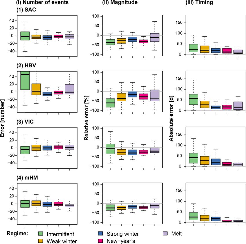
108                                                                             M. I. Brunner et al.: Model evaluation floods

0.69), over SAC (median EKG 0.63) and VIC (median EKG              for defining central tendencies of variables with a circular
0.60) to HBV (median EKG 0.52). In addition to streamflow,         behavior; Burn, 1997).
we use areal precipitation and simulated soil moisture to ex-
plain potential differences in model performance.                  2.2.3   Spatial flood dependence

2.2     Model evaluation for floods                                We then use the data sets resulting from Step 2 to evalu-
                                                                   ate how models reproduce overall and seasonal spatial flood
We compare local and spatial flood characteristics extracted       dependence. To do so, we use the connectedness measure
from the observed time series to those of the series sim-          introduced by Brunner et al. (2020a), which quantifies the
ulated with the four models for the period 1981–2008 for           number of catchments with which a specific catchment co-
the five streamflow regimes introduced above. Such a com-          experiences floods. The number of concurrent flood events
parison enables identification of flood characteristics whose      for a pair of stations is determined based on a data set consist-
model representation could potentially be improved. To bet-        ing of the dates of flood occurrences across all catchments.
ter understand potential model deficiencies, we look at how        This set is converted into a binary matrix which specifies
models capture flood triggering mechanisms and how they            for each catchment whether or not it is affected by a certain
simulate floods under climate conditions different from the        event. The matrix compiled using observed streamflow time
current ones.                                                      series contained 1164 events, among which 258 occur in win-
                                                                   ter, 291 in spring, 324 in summer, and 291 in fall. Following
2.2.1    Flood event identification                                the definition used by Brunner et al. (2020a), a catchment is
                                                                   connected to another catchment if they share a certain num-
Flood events are identified for each of the five time series       ber of events. We used here an event threshold of 1 % of the
(one observed, four simulated) using a peak-over-threshold         total or seasonal number of events to define connectedness
(POT) approach, similar to the one used in Brunner et al.          (all months: 12 events, seasons: 3 events). We computed ac-
(2019a, 2020b). This approach consists of two main steps           tual errors in flood connectedness by subtracting observed
and results in two data sets each, which are used for the lo-      from simulated connectedness over all seasons and per sea-
cal and spatial analysis, respectively: (1) POT events (i.e.,      son.
peak discharges) in individual catchments and (2) event oc-
                                                                   2.2.4   Flood triggers
currences across all catchments. In Step 1, independent POT
events are identified in the daily discharge time series of the    To explain potential differences in model performance, we
individual catchments using the 25th percentile of the corre-      look at the relationship of simulated peak discharge with the
sponding time series of annual maxima as a threshold (Schlef       two flood triggers precipitation and soil moisture on the day
et al., 2019) and by prescribing a minimum time lag of 10 d        of flood occurrence. We focus on the day of occurrence be-
between events (Diederen et al., 2019). This procedure re-         cause time of concentration is typically small for small head-
sults in a first quartile of 36, a median of 40, and a third       water basins (USDA-NRCS, 2010).
quartile of 47 events identified per basin.
   In Step 2, a data set consisting of the dates of flood oc-      2.2.5   Floods under change
currences across all catchments is compiled. This set is con-
verted into a binary matrix which specifies for each catch-        In addition to assessing model performance under current
ment (columns) whether or not it is affected by a specific         climate conditions, we would like to understand potential,
event (rows). We consider a catchment to be affected by a          additional challenges arising when interested in future con-
certain event if it experiences an event within a window of        ditions. To do so, we look at how models translate changes
±2 d of that event to take into account travel times. In addi-     in event temperature and precipitation into changes in POT
tion to a binary matrix of all events, we set up seasonal binary   discharge by performing a resampling-based sensitivity anal-
matrices (winter: December–February, spring: March–May,            ysis. This sensitivity analysis aims at evaluating whether a
summer: June–August, fall: September–November).                    model is still reliable under climate conditions different from
                                                                   the ones used in model calibration similar to split-sample or
2.2.2    Flood characteristics at individual sites                 differential split-sample calibration and validation schemes
                                                                   (Klemes, 1986; Coron et al., 2012; Refsgaard et al., 2014;
We use the data sets resulting from Step 1, the POT events         Thirel et al., 2015). To perform this sensitivity analysis, we
at individual catchments, to evaluate how well the models          generate surrogate time series of temperature, precipitation,
reproduce flood statistics at individual sites. We focus on the    and streamflow for each catchment (Wood et al., 2004; Brun-
total number of events n (actual error: ns − no , where “s”        ner et al., 2020b). To generate these series, we randomly sam-
represents simulations and “o” observations), magnitude in         ple a series of years with replacement in the period 1981–
terms of mean peak discharge x (relative error: (xs −xo )/xo ),    2008, which we use to compose time series consisting of
and mean timing (absolute error: circular statistics suitable      the daily values corresponding to these years for each of the

Hydrol. Earth Syst. Sci., 25, 105–119, 2021                                          https://doi.org/10.5194/hess-25-105-2021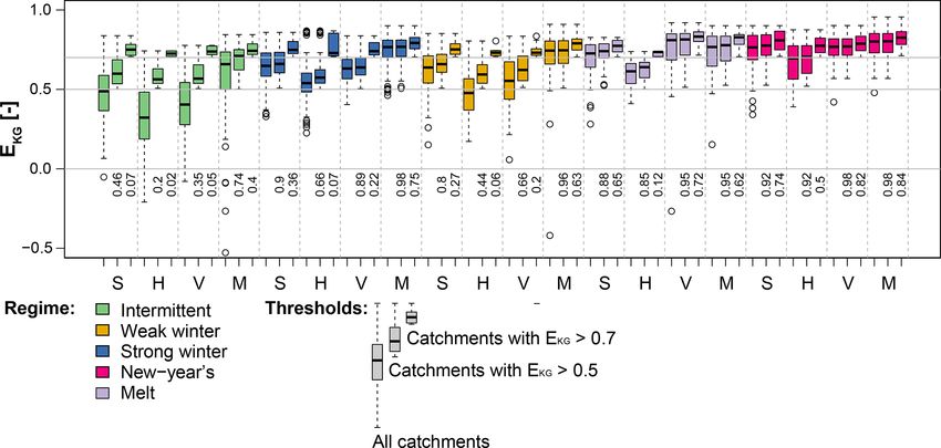
M. I. Brunner et al.: Model evaluation floods 109
Figure 2. Model performance in terms of EKG over the period 1981–2008 for the four models SAC (S), HBV (H), VIC (V), and mHM (M)
per hydrological regime: intermittent (114 catchments), weak winter (108), strong winter (176), New Year’s (50), and melt (40). For each
model and regime, three boxplots are shown: all catchments, catchments with EKG > 0.5, and catchments with EKG > 0.7. The percentage
[–] of catchments of a regime class above the corresponding threshold is indicated below the 0 line.
three variables. For each of the surrogate series, we again 3 Results
extract POT flood events using the same procedure as de-
scribed under Step 1. For each of the extracted events we 3.1 Flood characteristics at individual sites
then determine temperature and precipitation on the day of
peak discharge. We use the sets of peak discharge, event Model performance at individual sites with respect to the
temperature, and event precipitation to compute mean event number of events, event magnitude, and timing varies by
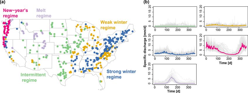
discharge, temperature, and precipitation, which enables the model and hydrological regime type (Fig. 3).
derivation of a relationship between mean POT discharge For most catchments, the median deviation between the
and the two meteorological variables during events. We re- simulated and observed number of flood events lies close to
peat the resampling n = 500 times to derive a relationship zero (SAC: −3 events, HBV: −1, VIC: −1, mHM: 0). How-
between changes in mean event temperature and precipita- ever, the simulations result in over- and underestimations
tion and changes in mean POT streamflow. This resampling of the number of events depending on the catchment (first
experiment results in a response surface of POT discharge and third quartiles for SAC: −9, 4; HBV: −8, 15; VIC: −7,
spanned by mean event temperature and mean event precipi- 6; mHM: −6, 6). The overestimation is strongest for HBV,
tation for each catchment. We summarize the results obtained which overestimates the number of events for catchments
at individual locations by computing horizontal and vertical with intermittent, weak winter, and melt regimes (Brunner
sensitivity gradients on these reaction surfaces using a lin- et al., 2020b). Event magnitude in terms of peak discharge is
ear regression model. The horizontal gradient describes the generally underestimated for all regime types independent of
strength of POT discharge changes in response to event tem- the model, and also absolute flood timing errors are present
perature changes, while the vertical gradient describes the in all models. They are the highest in catchments with in-
strength of change in response to changes in event precipita- termittent regimes with a high variability in flood timing and
tion. Conducting this experiment for both observed and sim- low in catchments with a New Year’s and melt regime, where
ulated time series allows for the determination of whether the flood season is limited to a few months (Brunner et al.,
the models react to changes in mean event temperature and 2020a).
precipitation in the same way as the real-world system and
are therefore suitable for use in climate change impact as- 3.2 Spatial flood dependencies
sessments of floods. If models produce different climate sen-
sitivities than the ones seen in the observations, the use of Over all seasons, most models show a median error close
models to simulate sets of flood events for future conditions to zero for flood connectedness. Flood connectedness can
may preclude reliable change assessments. be over- and underestimated dependent on the catchment
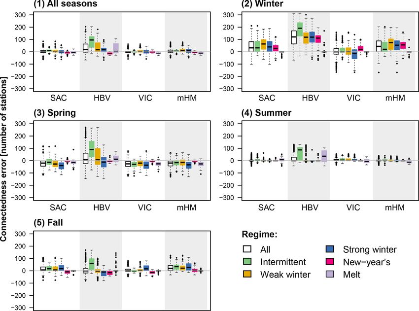
by most of the models, while HBV overestimates spatial
dependence in most catchments (Fig. 4). Seasonally, most
models over- or underestimate spatial dependence in cer-
tain regions. In winter, connectedness is overestimated by
most models except for VIC, and the strength of over-
https://doi.org/10.5194/hess-25-105-2021 Hydrol. Earth Syst. Sci., 25, 105–119, 2021110 M. I. Brunner et al.: Model evaluation floods
Figure 3. Model errors per regime type computed over the period 1981–2008: intermittent (114 catchments), weak winter (108), strong
winter (176), New Year’s (50), and melt (40) (Fig. 1). Errors are shown for (i) number of events (error in number of events), (ii) magnitude
(mean relative error), and (iii) timing (mean absolute error in days) for the four models (1) SAC, (2) HBV, (3) VIC, and (4) mHM. The
boxplots are composed of one value per catchment belonging to the respective regime class.
estimation is strongest for HBV. In spring, most models plus snowmelt; i.e., the higher the precipitation input or rain-
tend to underestimate spatial dependence except for HBV fall and snowmelt combined, respectively, the higher the re-
that results in an overestimation of spatial dependence for sulting peak discharge. This relationship is slightly more ex-
catchments with an intermittent regime. Connectedness over- pressed for VIC than for SAC. In both models, soil moisture
estimation by HBV is most pronounced for catchments and event magnitude are also positively related with lower
with an intermittent regime. Otherwise, connectedness over- peak values, potentially associated with lower soil mois-
/underestimation seems to be independent of the regime. ture states than more severe events. The peak discharge–
precipitation relationship of HBV and mHM is less straight-
3.3 Flood triggers forward than the one of SAC and VIC. HBV and mHM also
show high discharge when precipitation input is high but may
The differences in model performance regarding local and in some cases still produce high discharge values, even for
spatial flood characteristics may be partially explained by low precipitation inputs. Such low precipitation inputs can
differences in their structure and how they transform pre- also lead to high peak discharge for SAC but to a lesser
cipitation into runoff. Figure 5 shows how simulated peak degree than HBV and mHM. However, peak discharge and
discharge is related to event precipitation, event precipitation rainfall plus snowmelt show a strong linear relationship; i.e.,
plus snowmelt, and simulated soil moisture over all catch- the higher the combined rainfall and snowmelt input to the
ments for the four hydrologic models. The SAC and VIC system, the higher the peak discharge. High flows are in most
models show similar simulated relationships for all three cases related to nearly full storage states but can occasionally
variable pairs. There is a positive relationship between peak also be triggered when soil moisture is low for SAC and VIC
discharge and precipitation and peak discharge and rainfall and to a lesser degree for HBV.
Hydrol. Earth Syst. Sci., 25, 105–119, 2021 https://doi.org/10.5194/hess-25-105-2021M. I. Brunner et al.: Model evaluation floods 111
Figure 4. Overall (1) and seasonal (2–5) errors in flood connectedness (simulated minus observed connectedness), i.e., number of catchments
a catchment is sharing at least 1 % of the total number of flood events with, for the four models SAC, HBV, VIC, and mHM over all regimes
and per regime: intermittent (114 catchments), weak winter (108), strong winter (176), New Year’s (50), and melt (40).
3.4 Floods under change regime). In the case of melt regimes, the misrepresentation
of flood sensitivities by models suggests that they may have
In addition to looking at how well local and spatial flood difficulty simulating snow-influenced flooding.
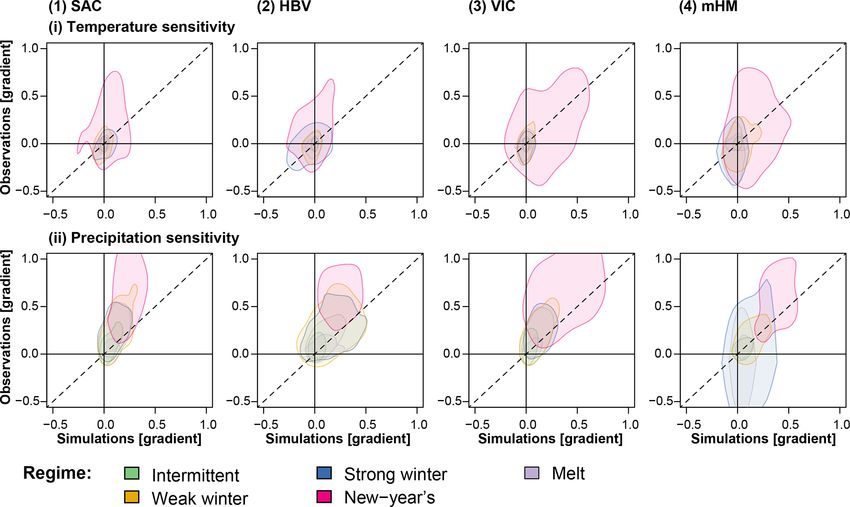
characteristics are represented by models, we look at how This relatively poor model performance in capturing ob-
changes in temperature and event precipitation are translated served flood sensitivities can be generalized to the larger set
into changes in flood flows to assess each model’s suitabil- of catchments studied here (Fig. 7). Temperature sensitivities
ity for climate impact assessments on floods. Our sensitiv- are found to be positive or negative; i.e., an increase in tem-
ity analysis shows that the models have difficulty translat- perature could lead to an increase or decrease of peak flow
ing changes in event temperature and precipitation into sen- depending on the catchment. In general, these temperature
sitivities of flood flows (Fig. 6), which can be problematic sensitivities are relatively weak (i.e., gradients are close to
if we would like to use such models in climate change as- zero), which may be the reason why they are difficult to cap-
sessments. Generally, flood flows show a relatively low sen- ture. In contrast, precipitation sensitivities are mostly posi-
sitivity to changes in mean event precipitation and temper- tive; i.e., an increase in event precipitation leads to an in-
ature. This is in contrast to the behavior for mean flow, crease in peak flow. However, the strength of these sensitivi-
which is strongly influenced by changes in mean precipita- ties is underestimated by all models; i.e., a change in precip-
tion as demonstrated in a similar experiment by Brunner et al. itation leads to too small a change in peak flow. This under-
(2020b). The much stronger relationship between mean pre- estimation of sensitivity can be understood by the underesti-
cipitation and flow than between event precipitation and flow mation of flood magnitude in general.
might arise because mean flow is a climate signal (Knoben
et al., 2018), whereas floods are more an event (higher fre-
quency, short-term) signal. However, some catchments, e.g., 4 Discussion
Tucca Creek (New Year’s regime), show a clear relationship
between peak magnitude and both event temperature and pre- 4.1 Model performance in simulating floods
cipitation. While these relationships are captured for some
catchments (e.g., Blackwater River, weak winter regime or The results presented in this study demonstrate that simulat-
Tucca Creek, New Year’s regime), they are not in other catch- ing floods using hydrological models calibrated on the pop-
ments. The simulated sensitivities may even point in another ular Kling–Gupta efficiency metric is challenging both at a
direction than the observed ones (e.g., Pacific Creek, melt local and spatial scale. At the local scale, flood timing and
https://doi.org/10.5194/hess-25-105-2021 Hydrol. Earth Syst. Sci., 25, 105–119, 2021112 M. I. Brunner et al.: Model evaluation floods Figure 5. Simulated relationships between normalized flood discharge (Q) and normalized precipitation (i; P ), rainfall and snowmelt (ii; R + M), and soil moisture (iii; SM, upper two soil layers for mHM) over all catchments represented by a binned scatter plot for the four hydrologic models (1) SAC, (2) HBV, (3) VIC, and (4) mHM. The darker the color, the higher the number of points within a bin (one point per catchment and event). Kendall’s correlation coefficients are provided in the upper right corners of the subplots. magnitude may not be perfectly captured, which can trans- ually results in an underestimation of peak flow (Mizukami late into a suboptimal representation of spatial dependencies et al., 2019) due to an underestimation of variability, which because space and time are closely related. The challenges will result in an underrepresentation of extremes (Katz and related to flood simulations become especially pronounced Brown, 1992). Another factor potentially contributing to this under climate conditions different from the current ones be- underestimation is that the models were forced with spa- cause additional sources of uncertainty are added to the mod- tially lumped instead of distributed data, which may have eling chain. smoothed the simulated discharge response. Even though the models have been calibrated for the lo- Under the current calibration paradigm, whereby models cal situation, substantial differences in magnitude and timing are calibrated to local discharge conditions using EKG as were found between observations and simulations. Locally, the objective function, flood connectedness is not accounted simulated floods showed smaller magnitudes and had differ- for. As a result, flood connectedness is not well captured by ent timing than observed ones, while the number of floods the models, as illustrated by the finding that flood connect- was reproduced relatively well except by the HBV model edness is over- or underestimated depending on the season. for catchments with intermittent regimes. The flood magni- The overestimation of spatial dependence in winter for all tude underestimation found for all four models tested is in regimes except the melt regime is likely related to higher line with previous studies showing that using EKG individ- simulated than observed snowmelt as high soil moisture and Hydrol. Earth Syst. Sci., 25, 105–119, 2021 https://doi.org/10.5194/hess-25-105-2021
M. I. Brunner et al.: Model evaluation floods                                                                                        113

Figure 6. Climate sensitivity analysis for the VIC model: dependence of mean POT magnitude (Q) on mean flood event precipitation (1 d;
P ) and mean flood temperature (T ) for five example catchments, those with the best EKG per regime type: intermittent regime (green; USGS
ID 09210500 Fontanelle Creek near Fontanelle, WY; EKG = 0.78), weak winter regime (yellow; USGS ID 02369800 Blackwater River near
Bradley, AL; EKG = 0.83), strong winter regime (blue; USGS ID 11522500 Salmon River above Somes, CA; EKG = 0.84), New Year’s
regime (pink; USGS ID 14303200 Tucca Creek near Blaine, OR; EKG = 0.9), and melt regime (purple; USGS ID 13011500 Pacific Creek
at Moran, WY; EKG = 0.92). Grid axes and grey scales differ between plots, where darker colors indicate higher flood magnitudes.

snow availability have been shown to increase spatial flood            generate surface runoff when precipitation intensity exceeds
connectedness (Brunner et al., 2020a). Related to this, the un-        infiltration capacity (Burnash et al., 1973; Liang et al., 1994).
derestimation of spatial connectedness in spring may be re-            In this case, incoming precipitation is directly translated into
lated to the subsequent missing snowmelt contributions. Spa-           flood discharge. In contrast, HBV and mHM, the latter of
tial connectedness in summer has been shown to be generally            which is based on the HBV model structure (Kumar et al.,
weak due to the occurrence of localized, convective events             2013), does not include a surface runoff component, and all
(Brunner et al., 2020a), which is reflected by most models             discharge originates in the model stores (Bergström, 1976).
except for HBV in the case of intermittent and melt regimes.           This introduces a nonlinearity in the model response and may
Spatial flood connectedness has also been shown to be weak             explain why a smaller precipitation input may still gener-
in fall (Brunner et al., 2020a) but is overestimated by most           ate high peak flows in these models. These differences in
models. The finding that there is room to improve the rep-             process representation suggest that a “most suitable model”
resentation of spatial flood dependencies is in line with pre-         could be identified for a specific application at hand. If one
vious studies showing that large-scale hydrological models             is, e.g., interested in simulating floods in catchments with in-
have a weakness in reproducing regional aspects of floods              termittent regimes, the HBV model does not seem to be an
(Prudhomme et al., 2011).                                              ideal choice because there it simulates too many floods with
   There are slight variations in performance among models.            too small a magnitude. The overestimation of the number of
These variations may result from differences in the repre-             events in catchments with intermittent regimes by HBV may
sentation of flood producing mechanisms, as indicated by               be explained by its fast response to precipitation as expressed
distinct behaviors in how the models translate precipitation           through its model parameter β, which introduces nonlinear-
into runoff. VIC and SAC show more linearity in their event            ity to the system (Viglione and Parajka, 2020).
precipitation and peak discharge relationship than HBV and                Our climate sensitivity analysis shows that the simulation
mHM, possibly because VIC and SAC have the capability to               of floods becomes even more challenging under climate con-

https://doi.org/10.5194/hess-25-105-2021                                                Hydrol. Earth Syst. Sci., 25, 105–119, 2021
114                                                                                    M. I. Brunner et al.: Model evaluation floods

Figure 7. Observed vs. simulated (i) horizontal (temperature) and (ii) vertical (precipitation) climate sensitivities for floods represented
by two-dimensional kernel density estimates for the four models (1) SAC, (2) HBV, (3) VIC, and (4) mHM for the five regime types:
intermittent (114 catchments), weak winter (108), strong winter (176), New Year’s (50), and melt (40) (Fig. 1). Positive and negative values
indicate positive and negative associations of precipitation and temperature with peak flow, respectively. Values on the dashed line indicate
correspondence between observed and modeled sensitivity gradients.

ditions different from the current ones as the hydrological              logic phenomena is likely to be improved by using more
models employed in this study have limited capability in                 tailored model calibration strategies. The representation of
reproducing observed hydrologic sensitivities during flood-              streamflow variability could potentially be improved by giv-
ing. These limitations may be related to input uncertainties             ing more weight to the variability component of an integra-
(Te Linde et al., 2007), insufficient model calibration (Fowler          tive metric such as the EKG (Pool et al., 2017), whereas the
et al., 2016), or equifinality in process contributions for sim-         representation of flood magnitude and timing may be im-
ulations with (very) similar efficiency scores, leading to an            proved by giving more weight to the bias and correlation
inability to unambiguously identify the appropriate relative             components of the EKG . Alternatively, these characteristics
process contributions (Khatami et al., 2019).                            could be optimized explicitly by minimizing the error in
                                                                         key hydrograph signatures related to site-specific flood phe-
4.2   Potential ways to improve model performance                        nomena. Such flood-focused optimization may similarly to
                                                                         EKG rely on multiple objectives in a scalar function (Gupta
                                                                         et al., 1998; Efstratiadis and Koutsoyiannis, 2010), such as
The results of our model comparison highlight that there is
                                                                         volume error, root-mean-squared error, and peak flow error
room for improvement regarding the representation of local
                                                                         (Moussa and Chahinian, 2009); ENS and relative peak devi-
flood events, spatial flood dependence, and flood producing
                                                                         ation (Krauße et al., 2012); EKG , peak efficiency, and loga-
mechanisms. We discuss here four potential ways for im-
                                                                         rithmic efficiency (Sikorska et al., 2018); or EKG , peak ef-
proving model performance: developing flood-tailored cali-
                                                                         ficiency, and mean absolute relative error (Sikorska-Senoner
bration metrics, considering spatial aspects in model calibra-
                                                                         et al., 2020). In addition, model performance can potentially
tion, improving representation of flood processes, and repre-
                                                                         be improved by using multiple metrics describing important
senting input uncertainties.
                                                                         catchment processes (Madsen, 2003; Dembélé et al., 2020),
   A first possibility to improve model performance is to de-
                                                                         i.e., flood generating mechanisms such as soil moisture and
velop calibration metrics tailored to flooding instead of re-
                                                                         snowmelt.
lying on EKG . Our results show that EKG can lead to sim-
                                                                            A second way to improve model performance is to fo-
ulation performance deficits for phenomena of interest, in-
                                                                         cus on the spatial representation of extremes, which may
cluding an underestimation of peak flow, a misrepresentation
                                                                         be improved by considering spatially distributed features of
of timing, and over- or underestimation of seasonal spatial
                                                                         model response or spatial correlation within a spatial cali-
flood connectedness. As is evident in some existing practice-
                                                                         bration framework. Such a framework could build upon ex-
oriented applications of hydrological models (Hogue et al.,
                                                                         isting spatial verification metrics such as the spatial predic-
2000; Unduche et al., 2018; World Meteorological Orga-
                                                                         tion comparison test used, e.g., to validate precipitation fore-
nization, 2011), the simulation of floods and other hydro-

Hydrol. Earth Syst. Sci., 25, 105–119, 2021                                                 https://doi.org/10.5194/hess-25-105-2021
M. I. Brunner et al.: Model evaluation floods 115 casts (SPCT; Gilleland, 2013), empirical orthogonal func- put uncertainty is particularly important if we are interested tions (EOFs), or Kappa statistics (Koch et al., 2015). For the in future changes because of climate model and scenario un- calibration and evaluation of spatially distributed hydrolog- certainty, where precipitation uncertainty is specifically pro- ical models, Koch et al. (2018) recently proposed the SPA- nounced (Chen et al., 2014; Lopez-Cantu et al., 2020). Even tial EFficiency (SPAEF) metric, which reflects three equally though many of these possibilities have been discussed in weighted components: correlation, coefficient of variation, previous studies, their consideration in flood analyses is not and histogram overlap. To improve the spatial dependence of standard practice. floods across different sites, such spatial calibration frame- works would need to include spatial verification metrics fo- cusing on extremes, which could, e.g., be achieved by look- 5 Conclusions ing at deviations of simulated from observed F-madograms, which measure extremal dependence (Cooley et al., 2012). Our model comparison shows that flood characteristics are Please note, however, that even the use of spatial verification not always well captured in hydrological models developed metrics may not overcome the lack of spatial heterogeneity for research studies – even when the models have been cal- in precipitation or soil moisture data. ibrated with a calibration metric perceived suitable for flood A third way of improving model performance is to test modeling, the Kling–Gupta efficiency metric (EKG ). The whether a model is fit for purpose and to identify model number of flood events was over- or underestimated depend- structures which accurately represent relevant flood produc- ing on the catchment, flood magnitudes were underestimated ing mechanisms. The importance of model structure choice by all models in most catchments, and the ability of the has been highlighted in previous studies both for low- and model to accurately reproduce event timing was proportional high-flow events (Melsen and Guse, 2019; Kempen et al., to the hydroclimatic seasonality. These model deficiencies 2020; Knoben et al., 2020) and should depend on the spa- in reproducing local flood characteristics, especially timing, tial complexity of the phenomenon studied (Hrachowitz and can lead to a misrepresentation of spatial flood dependencies, Clark, 2017). However, model structure choice for a spe- particularly in winter, because the temporal and spatial di- cific application is not straightforward, and automatic model mensions of flooding are closely linked. Our sensitivity anal- structure identification frameworks have only been intro- ysis also shows that climate sensitivities of floods, especially duced very recently (Spieler et al., 2020). To improve the rep- to changes in precipitation, are not well represented in mod- resentation of flood processes, such frameworks would ide- els, even if the model can be deemed “well calibrated” ac- ally explicitly consider local and spatial flood characteristics cording to the EKG metric. These sensitivities are generally and the representation of different flood generation processes underestimated by models independent of the geographical such as rain-on-snow events or flash floods. The representa- areas considered; i.e., an increase in event precipitation may tion of rain-on-snow floods for example requires an accurate not be translated into a strong enough increase in flood peak. representation of the energy balance in order to represent fac- The misestimation of these sensitivities may undermine the tors affecting snowmelt processes such as net radiation and reliability of future flood hazard assessments relying on such turbulent heat fluxes (Pomeroy et al., 2016; Li et al., 2019) . models. A fourth possibility to improve model performance is The limited capability of the models in reproducing local to address data uncertainty of streamflow observations and and spatial flood characteristics and the sensitivity of runoff of precipitation input. Errors in streamflow measurements to precipitation inputs is partly attributed to model struc- caused by stage–discharge rating-curve uncertainty (Coxon ture and partly to a reliance of the calibration on an indi- et al., 2015; Kiang et al., 2018) influence model calibration vidual variable (streamflow) and metric (EKG ). While EKG and evaluation. To improve uncertainty estimates, such un- is integrative of certain properties (bias, variance, correla- certainty should be accounted for by explicitly considering tion), it does nonetheless not explicitly focus on high-flow streamflow measurement uncertainty in model calibration values, their spatial dependencies, or processes generating (McMillan et al., 2010). In addition, the uncertainty of the high-flow values. We conclude that calibration using only an precipitation product used to drive a hydrological model can individual model performance metric or variable can result lead to differences in observed and simulated flows (Te Linde in model implementations that have limited value for spe- et al., 2007; Renard et al., 2011). Precipitation products cific model applications, such as local and in particular spa- may show observation uncertainties (Mcmillan et al., 2012) tial flood hazard analyses and change impact assessments. and underestimate extreme rainfall or the spatial dependence This study underscores the importance of improving the of extreme precipitation at different locations because spa- representation of magnitude, timing, spatial connectedness, tial smoothing or averaging during the gridding process re- and flood generating processes. Potential ways of achieving duces variability (Haylock et al., 2008; Risser et al., 2019). such improvements include developing flood-focused, multi- Such spatial uncertainty could be accounted for by using objective, and spatial calibration metrics, improving flood probabilistic analyses of precipitation fields (Newman et al., generating process representations through model structure 2015a; Frei and Isotta, 2019). The consideration of such in- comparisons, and reducing uncertainty in precipitation in- https://doi.org/10.5194/hess-25-105-2021 Hydrol. Earth Syst. Sci., 25, 105–119, 2021
116                                                                                   M. I. Brunner et al.: Model evaluation floods

put. Such steps are recommended to improve the reliability of           References
flood simulations and ultimately local and regional flood haz-
ard assessments under both current and future climate condi-            Addor, N. and Melsen, L. A.: Legacy, rather than adequacy, drives
tions.                                                                    the selection of hydrological models, Water Resour. Res., 55,
                                                                          378–390, https://doi.org/10.1029/2018WR022958, 2019.
                                                                        Anderson, E. A.: NOAA technical memorandum NWS-HYDRO-
                                                                          17: National Weather Service river forecast system-snow accu-
Data availability. Observed streamflow measurements were made
                                                                          mulation and ablation model, Tech. rep., U.S. Depertment of
accessible by the USGS and can be downloaded via the website at
                                                                          Commerce. National Oceanic and Atmospheric Administration,
https://waterdata.usgs.gov/nwis/uv/?referred_module=sw (USGS,
                                                                          National Weather Service, Washington, DC, 1973.
2019). Simulated streamflow, precipitation, and storage time se-
                                                                        Berghuijs, W. R., Allen, S. T., Harrigan, S., and Kirch-
ries can be requested from Lieke Melsen (lieke.melsen@wur.nl)
                                                                          ner, J. W.: Growing spatial scales of synchronous river
for the SAC, HBV, and VIC models and from Oldrich Rakovec
                                                                          flooding in Europe, Geophys. Res. Lett., 46, 1423–1428,
(oldrich.rakovec@ufz.de) for the mHM model.
                                                                          https://doi.org/10.1029/2018GL081883, 2019.
                                                                        Bergström, S.: Development and application of a conceptual runoff
                                                                          model for Scandinavian catchments. Swedish Meteorological
Supplement. The supplement related to this article is available on-       and Hydrological Institute (SMHI) RHO 7, Tech. Rep. January
line at: https://doi.org/10.5194/hess-25-105-2021-supplement.             1976, Sveriges Meteorologiska och Hydrologiska Institut, Nor-
                                                                          rköping, 1976.
                                                                        Bratley, P. and Fox, B. L.: Algorithm 659: Implement-
Author contributions. MIB and MPC developed the study design.             ing Sobol’s Quasirandom Sequence Generator, ACM Trans-
NM, OR, and LAM provided the model simulations and together               actions on Mathematical Software (TOMS), 14, 88–100,
with MIB, MPC, and WJMK interpreted the model output. AWW                 https://doi.org/10.1145/42288.214372, 1988.
assisted with the paper’s background and messaging and proposed         Brunner, M. I. and Sikorska, A. E.: Dependence of flood peaks
the climate sensitivity strategy. WK produced the model illustra-         and volumes in modeled runoff time series: effect of data
tions. MIB wrote the first draft of the paper, and all co-authors re-     disaggregation and distribution, J. Hydrol., 572, 620–629,
vised and edited the paper.                                               https://doi.org/10.1016/j.jhydrol.2019.03.024, 2018.
                                                                        Brunner, M. I., Furrer, R., and Favre, A.-C.: Modeling the spa-
                                                                          tial dependence of floods using the Fisher copula, Hydrol.
Competing interests. The authors declare that they have no conflict       Earth Syst. Sci., 23, 107–124, https://doi.org/10.5194/hess-23-
of interest.                                                              107-2019, 2019a.
                                                                        Brunner, M. I., Hingray, B., Zappa, M., and Favre, A. C.: Fu-
                                                                          ture trends in the interdependence between flood peaks and vol-
Acknowledgements. We thank the editor and the four reviewers for          umes: Hydro-climatological drivers and uncertainty, Water Re-
their constructive feedback, which helped to reframe and clarify the      sour. Res., 55, 1–15, https://doi.org/10.1029/2019WR024701,
storyline.                                                                2019b.
                                                                        Brunner, M. I., Gilleland, E., Wood, A., Swain, D. L., and
                                                                          Clark, M.: Spatial dependence of floods shaped by spa-
                                                                          tiotemporal variations in meteorological and land-surface
Financial support. This research has been supported by the Swiss
                                                                          processes, Geophys. Res. Lett., 47, e2020GL088000,
National Science Foundation via a Postdoc.Mobility grant (grant
                                                                          https://doi.org/10.1029/2020GL088000, 2020a.
no. P400P2_183844, granted to Manuela I. Brunner). We are grate-
                                                                        Brunner, M. I., Melsen, L. A., Newman, A. J., Wood, A. W., and
ful for co-author support by the Bureau of Reclamation (grant no.
                                                                          Clark, M. P.: Future streamflow regime changes in the United
CA R16AC00039), the US Army Corps of Engineers (grant no.
                                                                          States: assessment using functional classification, Hydrol. Earth
CSA 1254557), and the NASA Advanced Information Systems
                                                                          Syst. Sci., 24, 3951–3966, https://doi.org/10.5194/hess-24-3951-
Technology program (award ID 80NSSC17K0541). We also ac-
                                                                          2020, 2020b.
knowledge support from the Global Water Futures research pro-
                                                                        Burn, D. H.: Catchment similarity for regional flood frequency anal-
gram.
                                                                          ysis using seasonality measures, J. Hydrol., 202, 212–230, 1997.
                                                                        Burnash, R. J. C., Ferral, R. L., and McGuire, R. A.: A generalized
                                                                          streamflow simulation system. Conceptual modeling for digital
Review statement. This paper was edited by Nadav Peleg and re-            computers, Tech. rep., Joint Federal-State River Forecast Center,
viewed by four anonymous referees.                                        Sacramento, 1973.
                                                                        Chen, H., Sun, J., and Chen, X.: Projection and uncer-
                                                                          tainty analysis of global precipitation-related extremes
                                                                          using CMIP5 models, Int. J. Climatol., 34, 2730–2748,
                                                                          https://doi.org/10.1002/joc.3871, 2014.
                                                                        Clark, M. P., Wilby, R. L., Gutmann, E. D., Vano, J. A., Gangopad-
                                                                          hyay, S., Wood, A. W., Fowler, H. J., Prudhomme, C., Arnold,
                                                                          J. R., and Brekke, L. D.: Characterizing uncertainty of the hy-
                                                                          drologic impacts of climate change, Current Climate Change

Hydrol. Earth Syst. Sci., 25, 105–119, 2021                                                https://doi.org/10.5194/hess-25-105-2021
M. I. Brunner et al.: Model evaluation floods 117
Reports, 2, 55–64, https://doi.org/10.1007/s40641-016-0034-x, Harrigan, S., Zsoter, E., Alfieri, L., Prudhomme, C., Salamon,
2016. P., Wetterhall, F., Barnard, C., Cloke, H., and Pappenberger,
Cooley, D., Cisewski, J., Erhardt, R. J., Jeon, S., Mannshardt, E., F.: GloFAS-ERA5 operational global river discharge reanal-
Omolo, B. O., and Sun, Y.: A survey of spatial extremes: Mea- ysis 1979–present, Earth Syst. Sci. Data, 12, 2043–2060,
suring spatial dependence and modeling spatial effects, Revstat https://doi.org/10.5194/essd-12-2043-2020, 2020.
Statistical Journal, 10, 135–165, 2012. Hay, L., Norton, P., Viger, R., Markstrom, S., Steven Regan, R.,
Coron, L., Andréassian, V., Perrin, C., Lerat, J., Vaze, J., and Vanderhoof, M.: Modelling surface-water depression stor-
Bourqui, M., and Hendrickx, F.: Crash testing hydrological age in a Prairie pothole region, Hydrol. Process., 32, 462–479,
models in contrasted climate conditions: An experiment on https://doi.org/10.1002/hyp.11416, 2018.
216 Australian catchments, Water Resour. Res., 48, 1–17, Haylock, M. R., Hofstra, N., Klein Tank, A. M., Klok,
https://doi.org/10.1029/2011WR011721, 2012. E. J., Jones, P. D., and New, M.: A European daily high-
Coxon, G., Freer, J., Westerberg, I. K., Wagener, T., Woods, R., and resolution gridded data set of surface temperature and precipi-
Smith, P.: A novel framework for discharge uncertainty quantifi- tation for 1950–2006, J. Geophys. Res.-Atmos., 113, D20119,
cation applied to 500 UK gauging stations, Water Resour. Res., https://doi.org/10.1029/2008JD010201, 2008.
51, 5531–5546, https://doi.org/10.1002/2014WR016532, 2015. Hirpa, F. A., Salamon, P., Beck, H. E., Lorini, V., Alfieri, L., Zsoter,
Das, J. and Umamahesh, N. V.: Assessment of uncertainty in esti- E., and Dadson, S. J.: Calibration of the Global Flood Awareness
mating future flood return levels under climate change, Nat. Haz- System (GloFAS) using daily streamflow data, J. Hydrol., 566,
ards, 93, 109–124, https://doi.org/10.1007/s11069-018-3291-2, 595–606, https://doi.org/10.1016/j.jhydrol.2018.09.052, 2018.
2018. Hogue, T. S., Sorooshian, S., Gupta, H., Holz, A., and Braatz, D.:
De Luca, P., Hillier, J. K., Wilby, R. L., Quinn, N. W., and A multistep automatic calibration scheme for river forecasting
Harrigan, S.: Extreme multi-basin flooding linked with models, J. Hydrometeorol., 1, 524–542, 2000.
extra-tropical cyclones, Environ. Res. Lett., 12, 1–12, Hrachowitz, M. and Clark, M. P.: HESS Opinions: The
https://doi.org/10.1088/1748-9326/aa868e, 2017. complementary merits of competing modelling philosophies
Dembélé, M., Hrachowitz, M., Savenije, H. H. G., and Mar- in hydrology, Hydrol. Earth Syst. Sci., 21, 3953–3973,
iéthoz, G.: Improving the predictive skill of a distributed hy- https://doi.org/10.5194/hess-21-3953-2017, 2017.
drological model by calibration on spatial patterns with multi- Huang, S., Kumar, R., Rakovec, O., Aich, V., Wang, X., Samaniego,
ple satellite datasets, Water Resour. Res., 56, e2019WR026085, L., Liersch, S., and Krysanova, V.: Multimodel assessment
https://doi.org/10.1029/2019WR026085, 2020. of flood characteristics in four large river basins at global
Diederen, D., Liu, Y., Gouldby, B., Diermanse, F., and Voro- warming of 1.5, 2.0 and 3.0 K above the pre-industrial level,
gushyn, S.: Stochastic generation of spatially coherent river Environ. Res. Lett., 13, 124005, https://doi.org/10.1088/1748-
discharge peaks for continental event-based flood risk as- 9326/aae94b, 2018.
sessment, Nat. Hazards Earth Syst. Sci., 19, 1041–1053, Hundecha, Y. and Merz, B.: Exploring the relation-
https://doi.org/10.5194/nhess-19-1041-2019, 2019. ship between changes in climate and floods using a
Efstratiadis, A. and Koutsoyiannis, D.: One decade of model-based analysis, Water Resour. Res., 48, W04512,
multi-objective calibration approaches in hydrologi- https://doi.org/10.1029/2011WR010527, 2012.
cal modelling: a review, Hydrol. Sci. J., 55, 58–78, Katz, R. W. and Brown, B. G.: Extreme events in a changing cli-
https://doi.org/10.1080/02626660903526292, 2010. mate: variability is more important than averages, Clim. Change,
Fowler, K. J. A., Peel, M. C., Western, A. W., Zhang, L., 21, 289–302, 1992.
and Peterson, T. J.: Simulating runoff under changing cli- Keef, C., Tawn, J. A., and Lamb, R.: Estimating the proba-
matic conditions: Revisiting an apparent deficiency of concep- bility of widespread flood events, Environmetrics, 24, 13–21,
tual rainfall-runoff models, Water Resour. Res., 52, 1820–1846, https://doi.org/10.1002/env.2190, 2013.
https://doi.org/10.1111/j.1752-1688.1969.tb04897.x, 2016. van Kempen, G., van der Wiel, K., and Melsen, L. A.: The im-
Frei, C. and Isotta, F. A.: Ensemble spatial precipitation anal- pact of hydrological model structure on the simulation of ex-
ysis from rain gauge data: Methodology and application in treme runoff events, Nat. Hazards Earth Syst. Sci. Discuss.,
the European Alps, J. Geophys. Res.-Atmos., 124, 5757–5778, https://doi.org/10.5194/nhess-2020-154, in review, 2020.
https://doi.org/10.1029/2018JD030004, 2019. Khatami, S., Peel, M. C., Peterson, T. J., and Western, A. W.: Equi-
Gilleland, E.: Testing competing precipitation forecasts accurately finality and flux mapping: A new approach to model evalua-
and efficiently: The Spatial Prediction Comparison Test, Mon. tion and process representation under uncertainty, Water Resour.
Weather Rev., 141, 340–355, https://doi.org/10.1175/MWR-D- Res., 55, 8922–8941, https://doi.org/10.1029/2018WR023750,
12-00155.1, 2013. 2019.
Gupta, H. V., Sorooshian, S., and Yapo, P. O.: Toward improved Kiang, J. E., Gazoorian, C., McMillan, H., Coxon, G., Le Coz,
calibration of hydrologic models: Multiple and noncommensu- J., Westerberg, I. K., Belleville, A., Sevrez, D., Sikorska,
rable measures of information, Water Resour. Res., 34, 751–763, A. E., Petersen-Øverleir, A., Reitan, T., Freer, J., Renard, B.,
https://doi.org/10.1029/97WR03495, 1998. Mansanarez, V., and Mason, R.: A comparison of methods
Gupta, H. V., Kling, H., Yilmaz, K. K., and Martinez, G. F.: Decom- for streamflow uncertainty estimation, Water Resour. Res., 54,
position of the mean squared error and NSE performance criteria: 7149–7176, https://doi.org/10.1029/2018WR022708, 2018.
Implications for improving hydrological modelling, J. Hydrol., Klemes, V.: Operational testing of hydrological
377, 80–91, https://doi.org/10.1016/j.jhydrol.2009.08.003, 2009. simulation models, Hydrol. Sci. J., 31, 13–24,
https://doi.org/10.1080/02626668609491024, 1986.
https://doi.org/10.5194/hess-25-105-2021 Hydrol. Earth Syst. Sci., 25, 105–119, 2021You can also read