Verification of the Atmospheric Infrared Sounder (AIRS) and the Microwave Limb Sounder (MLS) ozone algorithms based on retrieved daytime and ...
←
→
Page content transcription
If your browser does not render page correctly, please read the page content below
Atmos. Meas. Tech., 14, 1673–1687, 2021
https://doi.org/10.5194/amt-14-1673-2021
© Author(s) 2021. This work is distributed under
the Creative Commons Attribution 4.0 License.

Verification of the Atmospheric Infrared Sounder (AIRS) and the
Microwave Limb Sounder (MLS) ozone algorithms based on
retrieved daytime and night-time ozone
Wannan Wang1,2,3 , Tianhai Cheng1 , Ronald J. van der A3 , Jos de Laat3 , and Jason E. Williams3
1 Aerospace Information Research Institute, Chinese Academy of Sciences, Beijing 100094, China
2 Universityof Chinese Academy of Sciences, Beijing 100049, China
3 Royal Netherlands Meteorological Institute (KNMI), De Bilt 3730 AE, the Netherlands

Correspondence: Tianhai Cheng (chength@radi.ac.cn)

Received: 19 May 2020 – Discussion started: 2 July 2020
Revised: 18 January 2021 – Accepted: 27 January 2021 – Published: 1 March 2021

Abstract. Ozone (O3 ) plays a significant role in weather and    ences, providing additional support for the retrieval method
climate on regional to global spatial scales. Most studies on    origin of AIRS in stratospheric column ozone (SCO) day–
the variability in the total column of O3 (TCO) are typi-        night differences. MLS day–night differences are dominated
cally carried out using daytime data. Based on knowledge         by the upper-stratospheric and mesospheric diurnal O3 cy-
of the chemistry and transport of O3 , significant deviations    cle. These results provide useful information for improving
between daytime and night-time O3 are only expected either       infrared O3 products.
in the planetary boundary layer (PBL) or high in the strato-
sphere or mesosphere, with little effect on the TCO. Hence,
we expect the daytime and night-time TCO to be very similar.
However, a detailed evaluation of satellite measurements of      1   Introduction
daytime and night-time TCO is still lacking, despite the exis-
tence of long-term records of both. Thus, comparing daytime      Atmospheric ozone (O3 ) is a key factor in the structure
and night-time TCOs provides a novel approach to verify-         and dynamics of the Earth’s atmosphere (London, 1980).
ing the retrieval algorithms of instruments such as the Atmo-    The 1987 Montreal Protocol on Substances that Deplete
spheric Infrared Sounder (AIRS) and the Microwave Limb           the Ozone Layer formally recognized the significant threat
Sounder (MLS). In addition, such a comparison also helps         of chlorofluorocarbons and other O3 -depleting substances
to assess the value of night-time TCO for scientific research.   (ODCs) to the O3 layer and marks the start of joint inter-
Applying this verification on the AIRS and the MLS data,         national efforts to reduce and ultimately phase-out the global
we identified inconsistencies in observations of O3 from both    production and consumption of ODCs (Velders et al., 2007).
satellite instruments. For AIRS, daytime–night-time differ-      Indeed, concerns about changes in O3 due to catalytic chem-
ences were found over oceans resembling cloud cover pat-         istry involving anthropogenically produced chlorofluorocar-
terns and over land, mostly over dry land areas, which is        bons has become an important topic for the scientific com-
likely related to infrared surface emissivity. These differ-     munity, the general public, and governments (Fioletov et al.,
ences point to issues with the representation of both pro-       2002).
cesses in the AIRS retrieval algorithm. For MLS, a major            In response to this concern and associated environmental
issue was identified with the “ascending–descending” orbit       policies, a large number of studies during the last 2 decades
flag, used to discriminate night-time and daytime MLS mea-       have focused on estimating long-term variations and trends
surements. Disregarding this issue, MLS day–night differ-        in the stratospheric column of O3 (SCO). A summary of the
ences were significantly smaller than AIRS day–night differ-     state of the science is frequently reported in the quadrennial
                                                                 O3 assessment reports issued by the United Nations Envi-

Published by Copernicus Publications on behalf of the European Geosciences Union.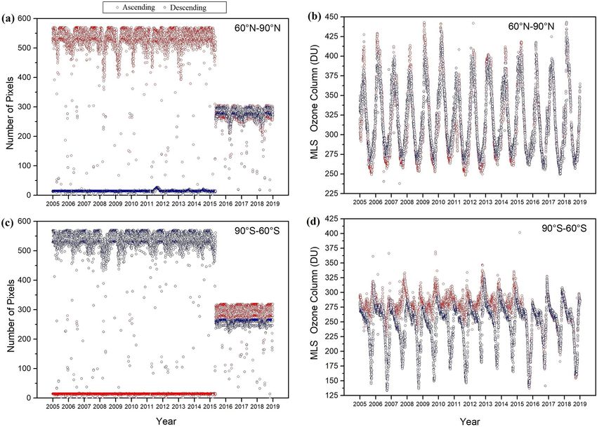
1674                                                    W. Wang et al.: Verification of the AIRS and MLS ozone algorithms

ronmental Programme (UNEP) and the World Meteorolog-               the total column of O3 (TCO). Hence, we expect the daytime
ical Organization (WMO). These reports are written in re-          and night-time TCO to be very similar. This slight variation
sponse to the global treaties aimed at minimizing the emis-        in diurnal TCO can serve as a natural test signal for remote
sion of ODSs. The signatories of these treaties ask for reg-       sensing instruments and data retrieval techniques. We need
ular updates on the state of the science and knowledge. The        to clarify how sensitive different space-based instruments are
most recent O3 assessment reports extensively discuss long-        to slight TCO changes, and we need to distinguish potential
term variations and trends in stratospheric O3 in relation         biases from retrieval artefacts. Day–night inter-comparisons
to expected recovery (WMO, 2011, 2014, 2018). Accord-              present a unique opportunity to assess the internal consis-
ing to WMO (2018), Antarctic stratospheric O3 has started          tency of infrared O3 instruments (Brühl et al., 1996; Pom-
to recover; moreover, outside of the polar regions, upper-         mier et al., 2012; Parrish et al., 2014). Systematic differences
stratospheric O3 has also increased. Conversely, no signif-        could potentially arise, for example, from temperature ef-
icant trend has been detected in global (60◦ S–60◦ N) total        fects within the instrument, from differences in signal mag-
column O3 over the 1997–2016 period, with average values           nitude between daytime and night-time, or from the retrieval
for the years since the last assessment remaining roughly          algorithms. The Stratosphere Aerosol and Gas Experiment
2 % below the 1964–1980 average. Furthermore, a debate             (SAGE) applied day–night differences to validate O3 profiles
has recently emerged over the question of whether lower-           and found that daytime values have a low bias due to errors in
stratospheric O3 between 60◦ S and 60◦ N has continued to          the retrieval method, as the magnitude of the difference was
decline despite decreasing O3 -depleting substances (Ball et       much less in a photochemical model (Cunnold et al., 1989).
al., 2018, 2019). In addition to the quadrennial O3 assess-        There are satellite instruments, like the Atmospheric Infrared
ments, the Bulletin of the American Meteorological Society         Sounder (AIRS) and the Microwave Limb Sounder (MLS),
(BAMS, American Meteorological Society, 2011) annually             that provide global daytime and night-time TCO or SCO and
publishes its “State of the Climate”; since 2015, this annual      O3 profiles. Although their daytime O3 retrievals have been
publication includes tropospheric O3 trends and effects from       validated (Livesey et al., 2008; Sitnov and Mokhov, 2016),
the El Niño–Southern Oscillation (ENSO), a description of          day–night differences in TCO and SCO are still largely unex-
the relevant stratospheric events of the past year, the state of   plored. By applying this day–night verification on the AIRS
the Antarctic O3 hole, and an annual update of global and          and MLS data, one can assess their capacities to characterize
zonal trends in stratospheric O3 . These regularly recurring       atmospheric O3 . Furthermore, an accurate assessment of O3
reports and publications illustrate the continued attention and    variation is needed for a reliable and homogeneous long-term
monitoring of the O3 layer and its recovery, in which the          trend detection in the global O3 distribution.
long-term records of satellite observations play a crucial role.      The O3 diurnal cycle depends on latitude, altitude,
Thus, establishing and maintaining the quality of the satellite    weather, and time. The variations in the diurnal cycle are
observations of stratospheric O3 is highly relevant.               less than 5 % in the tropics and subtropics and increase to
   A variety of techniques exist to measure the O3 col-            more than 15 % in the upper stratosphere during the polar
umn and stratospheric O3 . Ultraviolet (UV) absorption spec-       day near 70◦ N (Frith et al., 2020). Diurnal variations exist
troscopy with the sun or stars as sources of UV light is the       in atmospheric O3 at certain altitudes. There are two dis-
most commonly used method to derive O3 (Weeks et al.,              tinct O3 maxima in the typical vertical profile of the O3 vol-
1978; Fussen et al., 2000; Fu et al., 2013; Koukouli et al.,       ume mixing ratio: one in the lower stratosphere and one in
2015). In addition to the UV occultation method, the absorp-       the mesosphere. The secondary maximum in the mesosphere
tion of infrared radiation has also been used to detect O3 pro-    is present during both day and night (Evans and Llewellyn,
files throughout the column (Gunson et al., 1990; Brühl et al.,    1972; Hays and Roble, 1973). Chapman (1930) revealed the
1996). Another technique is the detection of the molecular         photochemical scheme in the mesosphere. The reactions of
oxygen dayglow emissions (Mlynczak and Drayson, 1990;              the Chapman cycle are important for us to understand diur-
Marsh et al., 2002). Some ground-based instruments use O3          nal O3 variation.
emissions in the microwave region to infer the O3 density
in the mesosphere (Zommerfelds et al., 1989; Connor et al.,        O2 + hv → 2O(λ < 240 nm),                                   (1)
1994). Infrared emission measurements overcome the limita-         O + O2 + M → O3 + M,
tions in the local time coverage of solar occultation and day-
glow technique, and their altitude resolution is significantly       (in which M stands for an air molecule)                   (2)
higher compared with microwave measurements (Kaufmann              O3 + O → 2O2 ,                                              (3)
et al., 2003). The strongest O3 infrared absorption centres        O3 + hv → O2 + O(λ < 1140 nm).                              (4)
near 9.6 µm.
   Based on knowledge of chemistry and transport of O3 , sig-      In the daytime mesosphere, catalytic O3 depletion by odd
nificant deviations between daytime and night-time O3 are          hydrogen has to be considered in addition to the Chapman
only expected either in the planetary boundary layer (PBL)         cycle. The anti-correlation of O3 and temperature is mainly
or high in the stratosphere or mesosphere, with little effect on   due to the temperature dependence of the chemical rate coef-

Atmos. Meas. Tech., 14, 1673–1687, 2021                                             https://doi.org/10.5194/amt-14-1673-2021
W. Wang et al.: Verification of the AIRS and MLS ozone algorithms                                                            1675

ficients (Craig and Ohring, 1958; Barnett et al., 1975). Huang      2     Data
et al. (2008, 1997) found midnight O3 increases in the meso-
sphere, based on SABER and MLS data respectively. Zom-              2.1    AIRS total column of O3 retrievals
merfelds et al. (1989) surmised that eddy transport may ex-
plain this increase, whereas Connor et al. (1994) stated that       The AIRS satellite instrument was the first in a new genera-
atmospheric tides are expected to cause systematic day–night        tion of high spectral resolution infrared sounder instruments
variations.                                                         flown aboard the National Aeronautics and Space Adminis-
   During daytime, photolysis is the major loss process. The        tration (NASA) Earth Observing System (EOS) Aqua satel-
main night-time O3 source in the mesosphere is atomic oxy-          lite (Aumann et al., 2003, 2020; Chahine et al., 2006; Di-
gen, whereas its sinks are atomic hydrogen and atomic oxy-          vakarla et al., 2008). The AIRS radiance data in the 9.6 µm
gen (Smith and Marsh, 2005). In addition to O3 chemical             band are used to retrieve column O3 and O3 profiles during
reactions with active hydrogen and molecular oxygen, the            both day and night (including the polar night) (Pittman et
turbulent mass transport also plays an important role in the        al., 2009; Fu et al., 2018; Susskind et al., 2003, 2011, 2014).
explanation of the secondary O3 maximum (Sakazaki et al.,           The AIRS V6 Level 3 daily standard physical retrieval prod-
2013; Schanz et al., 2014).                                         ucts (2003–2018) provide TCO and profiles of retrieved O3 .
   Tropospheric O3 is mainly produced during chemical re-           The daily Level 3 products comprise daily averaged measure-
actions when mixtures of organic precursors (CH4 and non-           ments on the ascending and descending branches of an orbit
methane volatile organic carbon, NMVOC), CO, and nitro-             with the quality indicators “best” and “good” and are binned
gen oxides (or NOx ) are exposed to the UV radiation in the         into 1◦ × 1◦ (latitude × longitude) grid cells. The O3 profile
troposphere (Simpson et al., 2014). At night, in the absence        is vertically resolved in 28 levels between 1100 and 0.1 hPa.
of sunlight, there is no O3 production, but surface O3 depo-        This makes it possible to compare SCO between AIRS and
sition and dark reactions transform the NOx –VOC mixture            MLS. Moreover, estimates of the errors associated with cloud
and remove O3 . The dark chemistry affects O3 , and its key         and surface properties are part of the AIRS V6 Level 2 stan-
ingredients mainly depend on the reactions of two nocturnal         dard physical retrieval product, which we used here to dis-
nitrogen oxides, NO3 (the nitrate radical) and N2 O5 (dini-         cuss further details. Outside of the polar zones (60–90◦ N and
trogen pentoxide). NO3 oxidizes VOCs at night, whereas the          90–60◦ S), ascending and descending correspond to daytime
reaction of N2 O5 with aerosol particles containing water re-       (13:30 LST, local solar time) and night-time (01:30 LST) re-
moves NOx . Both processes also remove O3 at night (Brown           spectively. Hereafter, we refer to “day” and “night” rather
et al., 2006).                                                      than ascending and descending between 60◦ S and 60◦ N.
   The diurnal cycle of O3 in the middle stratosphere had           In the polar zones, it is inappropriate to use the ascending
generally been considered small enough to be inconsequen-           (descending) mode to define daytime (night-time); therefore,
tial, with known larger variations in the upper stratosphere        we just compare differences between the ascending and de-
and mesosphere (Prather, 1981; Pallister and Tuck, 1983).           scending mode. AIRS TCO measurements agree well with
Later studies have highlighted observed and modelled peak-          the global Brewer–Dobson network station measurements
to-peak variations of the order of 5 % or more in the mid-          with a bias of less than 4 % and a root-mean-square error
dle stratosphere between 30 and 1 hPa (Sakazaki et al., 2013;       (RMSE) difference of approximately 8 % (Divakarla et al.,
Parrish et al., 2014; Schanz et al., 2014).                         2008; Nalli et al., 2018; Smith and Barnet, 2019). Analysis
   In terms of dynamics, vertical transport due to atmospheric      of AIRS TCO monthly maps revealed that its retrievals de-
tides is expected to contribute to diurnal O3 variations at alti-   pict seasonal trends and patterns in concurrence with Ozone
tudes where background O3 levels have a sharp vertical gra-         Monitoring Instrument (OMI) and Solar Backscatter Ultra-
dient (Sakazaki et al., 2013). The Brewer–Dobson circula-           violet Radiometer (SBUV/2) observations (Divakarla et al.,
tion transports air upwards in the tropics, and polewards and       2008; Tian et al., 2007).
downwards at high latitudes, with stronger transport towards
the winter pole (Chipperfield et al., 2017).                        2.2    MLS stratospheric column of O3 and O3 profile
   The main objective of this paper is to analyse day–night                retrievals
differences in the AIRS TCO and the MLS SCO as well as
in MLS upper atmospheric O3 profiles. Section 2 discusses           The MLS instrument on-board the Aura satellite, which was
the data used. Section 3 presents results for AIRS, MLS,            launched on 15 July 2004 and placed into a near-polar Earth
the comparison of AIRS with MLS, and an application of              orbit at 705 km with an inclination of 98◦ , uses the mi-
AIRS TCO data over the Pacific low-O3 regions to highlight          crowave limb-sounding technique to measure vertical pro-
how day–night differences affect the use and interpretation         files of chemical constituents and dynamical tracers between
of TCO data. Finally, Sect. 4 provides a brief summary and          the upper troposphere and the lower mesosphere (Waters et
conclusions.                                                        al., 2006). Its orbital ascending mode is at 13:42 LST and
                                                                    the orbital descending mode is at 01:42 LST between 60◦ S
                                                                    and 60◦ N. In this study, we use the MLS v4.2x standard O3

https://doi.org/10.5194/amt-14-1673-2021                                             Atmos. Meas. Tech., 14, 1673–1687, 2021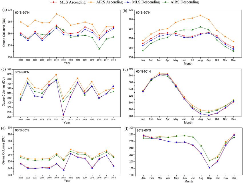
1676                                                     W. Wang et al.: Verification of the AIRS and MLS ozone algorithms

product during 2005–2018. Its retrieval uses 240 GHz radi-          (Feltz et al., 2018). Figure 1f shows absolute differences be-
ance and provides near-global spatial coverage (82◦ S–82◦ N         tween all subsequent pixels in the longitudinal direction. The
latitude), with each profile spaced 1.5◦ or ∼ 165 km along          figure reveals significant non-physical TCO changes (discon-
the orbit track. This O3 product includes the O3 profile on         tinuities) for adjacent land–ocean pixels (visible at coast lines
55 pressure surfaces, and the recommended useful vertical           running in the north–south direction). All of these effects
range is from 261 to 0.02 hPa. In addition, it contains an O3       are important parameters for the retrieval algorithm, but they
column, which is the integrated stratospheric column down           bear no physical relation to total O3 . The observed diurnal
to the thermal tropopause calculated from MLS-measured              cycle in AIRS TCO is related to either the measurements or
temperature (Livesey et al., 2015). Jiang et al. (2007) found       to the algorithm. If the diurnal cycles in AIRS TCO are re-
that the MLS stratospheric O3 data between 120 and 3 hPa            lated to the retrieval algorithm, it has to be caused by the
agreed well with ozonesonde measurements, within 8 % for            representation of a process in the algorithm having a diurnal
the global daily average. Froidevaux et al. (2008) reported         cycle; Smith and Barnet, 2019) argue that the issue does not
MLS stratospheric O3 uncertainties of the order of 5 %, with        stem from the algorithm but should be taken into account.
values closer to 10 % (and occasionally 20 %) at the low-           Hence, the differences shown in Fig. 1 provide strong indi-
est stratospheric altitudes. Livesey et al. (2008) estimated the    cations that the largest AIRS day–night TCO differences are
MLS O3 accuracy as ∼ 40 ppbv ± 5 % (∼ 20 ppbv ± 20 % at             dominated by retrieval artefacts. As such, changes are un-
215 hPa). Expectations and comparisons with other observa-          physical, and this confirms the hypothesis that clouds and the
tions show good agreements for the MLS O3 product, which            surface type (land, desert, vegetation, snow, or ice) affect the
are generally consistent with the systematic errors quoted          AIRS TCO retrievals. Note that TCO day–night differences
above.                                                              over land could also be (partly) related to clouds.
                                                                       The AIRS emissivity retrieval uses the NOAA regres-
                                                                    sion emissivity product as a first guess over land. The
3     Results                                                       NOAA approach is based on clear radiances simulated from
                                                                    the European Centre for Medium-Range Weather Forecasts
3.1    AIRS O3 retrievals’ day–night differences                    (ECMWF) forecast and a surface emissivity training data set
                                                                    (Goldberg et al., 2003). The training data set used for the
Figure 1 shows spatial variations in the differences between        AIRS V4 algorithm has a limited number of soil, ice, and
the AIRS day and night measurements. Generally, over 90 %           snow types and very little emissivity variability in the train-
of the globe, AIRS TCO is smaller during night-time than            ing ensemble. In the AIRS V5 version, the regression coef-
during daytime. The reduction of AIRS TCO over land at              ficient set has been upgraded using a number of published
night is greater than over oceans depending on the surface          emissivity spectra (12 spectra for ice and/or snow and 14 for
type. The seasonal averaged O3 day-to-night relative differ-        land) blended randomly for land and ice (Zhou et al., 2008).
ence shown in Fig. 1a–d reveals that AIRS TCO day and               These improvements generated a better emissivity first guess
night difference variations in Asia, Europe, and North Amer-        for use with the AIRS V5 and improved retrievals over the
ica during winter in the Northern Hemisphere (DJF) are              desert regions (Divakarla et al., 2008). In AIRS V6, a surface
smaller than during summertime (JJA), which is in line with         climatology was constructed from the 2008 monthly MODIS
the efficiency of photochemical production between seasons          MYD11C3 emissivity product and was extended to the AIRS
in the Northern Hemisphere. The Sahara Desert shows a               IR frequency hinge points using the baseline-fit approach
maximum difference value during wintertime, when there              described by Seemann et al. (2008). Note that AIRS obser-
are large day–night temperature differences. The same phe-          vations with low information content (especially around the
nomenon is observed in Western Australia during summer-             poles) will be drawn to the AIRS a priori value. This AIRS
time. The fact that the presence of a day–night difference ap-      a priori value for O3 is a climatology without diurnal varia-
pears to correlate with surface infrared emissivity properties      tion. If either the day or night observation has a lower infor-
of dry desert regions is consistent with Masiello et al. (2014),    mation content than the other, this too can result in a day–
who discussed the variability of surface infrared emissivity in     night difference. This is probably the reason for the differ-
the Sahara Desert and recommended taking the diurnal varia-         ences in Fig. 1 over pole ice. Nevertheless, using day–night
tion in the surface emissivity into account in infrared retrieval   differences for the evaluation of the AIRS V6 O3 product
algorithms.                                                         suggests that further refinements for better surface emissivity
   Figure 1e shows the annual mean large differences of             retrievals are required and that issues related to cloud cover
AIRS TCO retrievals over deserts, difference patterns over          need to be solved.
the oceans associated with the Intertropical Convergence
Zone (ITCZ), as well as regions with persistent seasonal sub-       3.2   MLS O3 retrievals’ day–night differences
tropical stratocumulus fields. The spatial patterns over land
mimic regions with low IR surface emissivity and/or regions         In order to better understand day–night differences in TCO,
where IR surface emissivity exhibits large seasonal variations      we also study day–night changes in the vertical profile of

Atmos. Meas. Tech., 14, 1673–1687, 2021                                              https://doi.org/10.5194/amt-14-1673-2021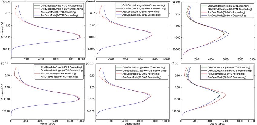
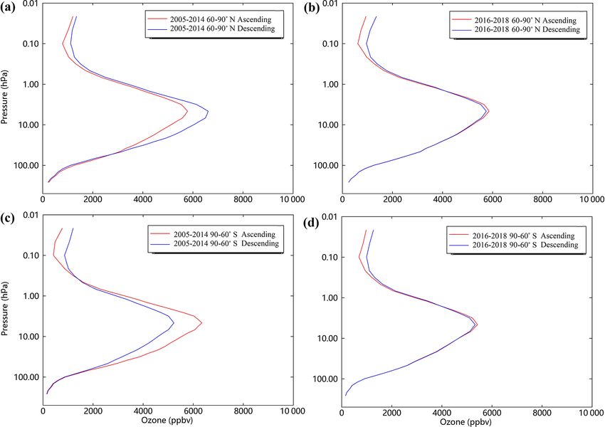
W. Wang et al.: Verification of the AIRS and MLS ozone algorithms                                                                          1677

Figure 1. AIRS TCO averaged day-to-night relative difference during 2003–2018 for (a) December–January–February, (b) March–April–
May, (c) June–July–August, and (d) September–October–November. (e) AIRS TCO 16-year averaged day-to-night relative difference during
2003–2018. (f) Absolute difference between two adjacent pixels at the same latitude in panel (e). Note that the relative difference is calculated
as 100 × (daytime − night-time) / daytime (in percent, %).

O3 using MLS O3 profile measurements. There are two                           We find an unexpected polar bias distinguished by the “As-
ways to distinguish between day and night in the observa-                  cDescMode” flag at high latitudes in Fig. 2c and f. On the
tions. When the observation mode is ascending (day), the pa-               one hand, the larger differences between the ascending and
rameter “AscDescMode” is set to 1; when it is descending                   descending MLS O3 profiles at high latitude extend from the
(night), the parameter “AscDescMode” is set to −1. Alter-                  stratosphere to the mesosphere; on the other hand, ascending
natively, the “OrbitGeodeticAngle” parameter of the prod-                  O3 is smaller than descending O3 at 10 hPa between 60 and
uct embeds the same information, expressed as an angle                     90◦ N in Fig. 2c, which is in contrast with the result of other
(Nathaniel J. Livesey, personal communication, 2020).                      latitudinal bands.
   Figure 2 shows that the global (60◦ S–60◦ N) differences                   Day and night MLS O3 profiles distinguished by the “Or-
between the day and night MLS O3 profile occur in the meso-                bitGeodeticAngle” flag at different latitude bands (30◦ ) be-
sphere (10–0.1 hPa). The O3 mixing ratios are about an order               tween 60◦ S and 60◦ N display same results as analysis by
of magnitude larger during night in the mesosphere, which                  “AscDescMode”. Figure 2c and f show that the varieties of
was previously revealed by Huang et al. (2008).                            ascending and descending MLS O3 profiles distinguished by

https://doi.org/10.5194/amt-14-1673-2021                                                       Atmos. Meas. Tech., 14, 1673–1687, 2021
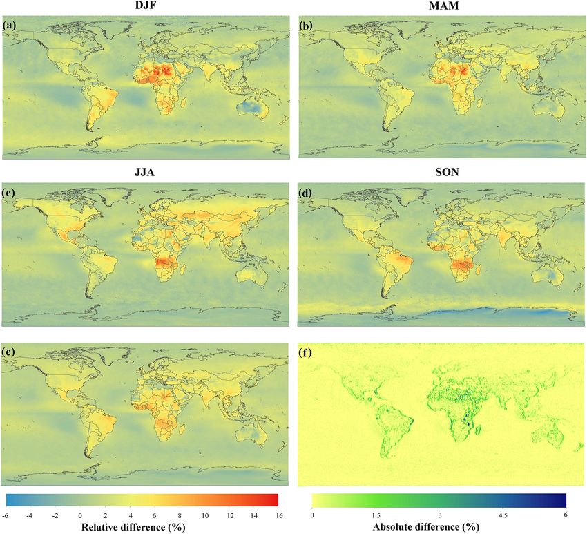
1678                                                   W. Wang et al.: Verification of the AIRS and MLS ozone algorithms

Figure 2. Ascending and descending MLS ozone profile between 261 and 0.02 hPa per latitude band (30◦ ) for 2005–2018: (a) 0–30◦ N,
(b) 30–60◦ N, (c) 60–90◦ N, (d) 30◦ S–0, (e) 60–30◦ S, and (f) 90–60◦ S.

the “OrbitGeodeticAngle” flag at high latitudes are consis-        in this study, released in February 2015, was generally sim-
tent with other regions.                                           ilar to the previous version. One of the major improvements
   The MLS O3 profile polar bias mentioned above turns out         of MLS v4.2x was the handling of contamination from cloud
to be related to an inconsistency in the “AscDescMode” flag        signals in trace gas retrievals that resulted in a significant re-
of the MLS v4.20 standard O3 product between 90 and 60◦ S          duction in the number of spurious MLS profiles in cloudy re-
and between 60 and 90◦ N. In version v4.22 and later ver-          gions and a more efficient screening of cloud-contaminated
sions this has been fixed. Figure 3a and c show that there         measurements. Furthermore, the MLS O3 products have been
is a clear change in the daily number of ascending and de-         improved through additional retrieval phases and a reduction
scending pixels on 14 May 2015, which is consistent with the       in interferences from other species (Livesey et al., 2015).
change in MLS SCO in Fig. 3b and d. After 14 May 2015 (us-
ing version v4.22), the ascending and descending MLS SCO           3.3   Comparison between AIRS and MLS O3 retrievals
are much closer. For the MLS O3 profile in Fig. 4, differences
between ascending and descending MLS O3 profiles at high           Figure 5 presents comparison of yearly and monthly aver-
latitudes for 2016–2018 are very small. Note that the con-         aged SCO for 2005–2018 observed by AIRS and MLS in
cept day–night has less physical relevance in polar regions        three latitude bands. Figure 5 explores the seasonality of ei-
due to the presence of the polar day or night. Outside of polar    ther AIRS or MLS SCO day–night differences as well as
regions many atmospheric parameters show significant 24 h          whether the seasonality in day–night SCO varies in uni-
cyclic changes due to differences in heating and cooling be-       son over the seasons. Figure 5a shows the 14-year aver-
tween day and night. Due to Earth’s orbital inclination, 24 h      age daytime AIRS SCO (250–1 hPa) and MLS SCO (261–
cyclic variations in atmospheric parameters in polar regions       0.02 hPa) between 60◦ S and 60◦ N for 2005–2018. The
are less significant or even absent.                               time-averaged MLS SCO column is 260.62 DU and AIRS
   The O3 retrieval algorithm adopted by the MLS v2.2              SCO is 264.24 DU. The average MLS SCO day–night differ-
products has been validated to be highly accurate using            ences for 2005–2018 (0.88 DU) are smaller than the AIRS
multiple correlative measurements, and the data have been          SCO day–night differences observed for the same time pe-
widely used (Jiang et al., 2007; Froidevaux et al., 2008).         riod (5.24 DU). The day–night difference of MLS SCO is
The MLS v3.3 and v3.4 O3 profiles were reported on a finer         0.79 DU in the mesosphere (10–0.1 hPa) and 0.03 DU in
vertical grid, and the bottom pressure level with scientif-        the stratosphere (100–10 hPa). The day–night difference of
ically reliable values (MLS O3 accuracy was estimated at           AIRS SCO is 1.51 DU in the mesosphere (10–1 hPa) and
∼ 20 ppbv + 10 % at 261 hPa) increases from 215 to 261 hPa         3.85 DU in the stratosphere (100–10 hPa). Compared with
(Livesey et al., 2015). The latest MLS v4.2x O3 profile used       the AIRS SCO day–night differences, the magnitudes of

Atmos. Meas. Tech., 14, 1673–1687, 2021                                              https://doi.org/10.5194/amt-14-1673-2021
W. Wang et al.: Verification of the AIRS and MLS ozone algorithms                                                             1679

Figure 3. (a) Time series of daily number of ascending and descending pixels between 60 and 90◦ N. (b) Time series of daily average
ascending and descending MLS SCO between 60 and 90◦ N. Panel (c) is the same as panel (a) but for 90–60◦ S. Panel (d) is the same as
panel (b) but for 90–60◦ S.

MLS SCO day–night differences in the stratosphere and in            ice). Therefore, the monthly 14-year average daytime AIRS
the mesosphere are much smaller. It has been pointed out            SCO and MLS SCO in Fig. 5d and f show similar patterns.
that errors in temperature profiles and water vapour mixing         Figure 5c–f confirm that both MLS and AIRS can catch SCO
ratios will adversely affect the AIRS O3 retrieval. Significant     seasonality at high latitudes. For AIRS SCO in Fig. 5f, the
biases (0 %–100 %) may exist in the region between ∼ 300            smallest day–night differences occur in September during the
and ∼ 80 hPa (Wang et al., 2019; Olsen et al., 2017). AIRS          Antarctic O3 hole.
O3 retrievals do not distinguish portions of the O3 profile as
being of different qualities, because all AIRS O3 channels          3.4   Day–night difference of equatorial Pacific low-O3
sense the surface as well as atmospheric O3 . Thus, AIRS O3               regions
retrievals are compromised if the surface is not well charac-
terized (Olsen et al., 2017). In addition, AIRS SCO retrievals      Generally, the Pacific low-O3 region (TCO < 220 DU),
show smaller day–night differences in the polar zones (1–           called the zonal wave-one feature (Newchurch et al., 2001;
2 DU) than between 60◦ S and 60◦ N (4–5 DU). This is re-            Ziemke et al., 2011), exists all year round. It is caused by
lated to clouds and the surface type which both affect the          lower NOx concentrations in this region. Other causes are
AIRS O3 retrievals as mentioned above. Figure 5b shows the          tropospheric O3 loss related to higher air temperatures and
monthly 14-year average daytime AIRS SCO and MLS SCO                higher water concentrations. High sea surface temperatures
between 60◦ S and 60◦ N for 2005–2018. Seasonal or random           favour strong convective activity in the tropical western Pa-
changes in clouds and the surface emissivity have a more sig-       cific, which can lead to low O3 mixing ratios in the convec-
nificant impact on each monthly AIRS SCO retrieval than on          tive outflow regions in the upper troposphere in spite of the
the MLS SCO retrieval. Compared with the 60◦ S–60◦ N re-            increased lifetime of odd oxygen (Kley et al., 1996; Rex et
gion, surface types in polar zones are less diverse (snow or        al., 2014). A further reduction in the tropospheric O3 burden

https://doi.org/10.5194/amt-14-1673-2021                                              Atmos. Meas. Tech., 14, 1673–1687, 2021
1680 W. Wang et al.: Verification of the AIRS and MLS ozone algorithms
Figure 4. (a) Averaged MLS ozone profile between 261 and 0.02 hPa for 2005–2014 from 60 to 90◦ N. (b) Averaged MLS ozone profile
between 261 and 0.02 hPa for 2016–2018 from 60 to 90◦ N. Panels (c) is the same as panel (a) but for 90–60◦ S. Panel (d) is the same as
panel (b) but for 90–60◦ S.
through bromine and iodine emitted from open-ocean ma- of the low-O3 regions is based on only a few observations.
rine sources has been postulated by numerical models (Vogt We cannot distinguish whether it is an algorithm problem
et al., 1999; von Glasow et al., 2002, 2004; Yang et al., 2005) or a chemical mechanism that caused this phenomenon. For
and observations (Read et al., 2008). However, the day–night AIRS, clouds over oceans may have greater impact on the
differences in this region are expected to be small. AIRS TCO retrievals at night. For MLS, more active chemi-
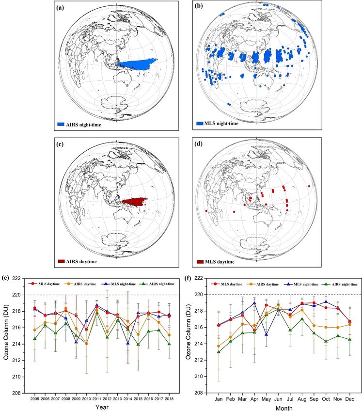
Figure 6a and c show that the low-O3 region is mainly lo- cal reactions may occur in these low-O3 regions at night.
cated over the western Pacific by AIRS. Rajab et al. (2013) For past, current, and future monitoring of atmospheric
investigated similar low TCO in Malaysia using AIRS data. phenomena like the Pacific tropospheric low-O3 area, it is
They found that the highest O3 concentration occurred in important that observations are sufficiently accurate. The
April and May, and the lowest O3 concentration occurred evaluation of day–night differences in both MLS and AIRS
during November and December, which is consistent with has revealed the existence of biases in the satellite data that
our results in Fig. 6f. They also found that O3 concentra- are large enough in comparison to expected variations and
tions exhibited an inverse relationship with rainfall but were changes in atmospheric O3 that they may hamper the use of
positively correlated with temperature. Figure 6b shows that, these satellite data studying them.
in addition to the tropical western Pacific, low-O3 regions for
MLS appear all over the tropical zone (30◦ S–30◦ N) at night.
However, Fig. 6d shows that the occurrence frequency and 4 Conclusions
intensity of daytime low-O3 regions by MLS SCO retrievals
drastically reduces and exists mainly in tropical western Pa- Comparison of daytime and night-time AIRS TCO has re-
cific. In Fig. 6e and f, yearly and monthly averaged AIRS vealed small but not insignificant biases in AIRS TCO. The
TCO and MLS SCO of the low-O3 regions show no con- differences are likely related to surface type (land, desert,
sistency or regularity. The analysis of daytime MLS SCO vegetation, snow, or ice) and infrared surface emissivity, es-
pecially over regions that exhibit smaller infrared emissiv-
Atmos. Meas. Tech., 14, 1673–1687, 2021 https://doi.org/10.5194/amt-14-1673-2021W. Wang et al.: Verification of the AIRS and MLS ozone algorithms 1681 Figure 5. Yearly and monthly averaged AIRS SCO and MLS SCO for 2005–2018. AIRS SCOs are calculated from 250 to 1 hPa. ity or large seasonal variability in infrared emissivity. Differ- for surface temperature and emissivity over land and ice sur- ences were typically of the order of a few percent, which is faces compared with previous versions. Nevertheless, our re- significant given that long-term changes in TCOs related to sults indicate that the AIRS V6 TCO still can be further im- anthropogenic emissions of stratospheric O3 -depleting sub- proved with respect to the representation of infrared emissiv- stances outside of polar regions are also of the order of a few ity. In addition, AIRS TCO differences over oceans bear a percent. clear cloud cover signature, which is likely related to uncer- Over land, patterns in day–night differences appear to be tainties in the representation of clouds in the retrieval algo- dominated by the dryness of the surface, suggesting that rithm. The latter may also impact AIRS TCO retrievals over emissivity may not be well represented or that reduced sen- land, although detection of cloud features in AIRS TCO day– sitivity to the lower troposphere during night compared with night differences over land is difficult due to the presence of day over hot surfaces results in a different AIRS TCO. The the land surface emissivity-related bias. spatial inhomogeneity of day–night AIRS TCO differences For ocean regions with persistent clouds during day and over drier regions points to emissivity dominating these dif- night (for example, over the ITCZ), Fig. S1 in the Sup- ferences. Infrared satellite retrieval artefacts due to land sur- plement shows that variations in cloud layer height have face emissivity is a well-known phenomenon (Zhou et al., a greater impact on AIRS TCO day–night differences than 2013; George et al., 2015; Bauduin et al., 2017). variations in the cloud fraction. There were major changes to the surface emissivity re- Our results do not provide much evidence of another pos- trieval in AIRS V6 compared with previous versions, result- sible causes of day–night differences in AIRS TCO: the pho- ing in a very significant improvement in yield and accuracy tochemical diurnal O3 cycle in the lower troposphere and up- https://doi.org/10.5194/amt-14-1673-2021 Atmos. Meas. Tech., 14, 1673–1687, 2021
1682                                                      W. Wang et al.: Verification of the AIRS and MLS ozone algorithms

Figure 6. Spatial and temporal distribution of the low ozone. (a) Location (composite pixel) of the yearly night-time low ozone from 2005
to 2018 for AIRS TCO. Panel (b) is the same as panel (a) but for MLS SCO. (c) Location (composite pixel) of the yearly daytime low ozone
from 2005 to 2018 for AIRS TCO. Panel (d) is the same as panel (c) but for MLS SCO. (e) Yearly averaged AIRS TCO and MLS SCO of the
low-ozone regions for 2005–2018. (f) Monthly averaged AIRS TCO and MLS SCO of the low-ozone regions for 2005–2018. Uncertainties
represent the standard deviation of the measured values.

per atmosphere. The strongest diurnal O3 effects occur in the          tion and a general slow O3 destruction regime (∼ 10 % d−1 ).
boundary layer over land due to night-time surface deposi-             Similarly, in the free troposphere, the diurnal O3 cycle is also
tion and daytime photochemical O3 production in the pres-              weak due to low O3 production rates (generally low levels
ence of air pollution. In the marine boundary layer, the diur-         of pollution relevant for O3 production). Hence, the diurnal
nal O3 cycle is much weaker due to the absence of air pollu-           O3 cycle in the free troposphere above 750 hPa is negligible

Atmos. Meas. Tech., 14, 1673–1687, 2021                                                  https://doi.org/10.5194/amt-14-1673-2021
W. Wang et al.: Verification of the AIRS and MLS ozone algorithms                                                                   1683

(Petetin et al., 2016). In summary, any tropospheric photo-           Supplement. The supplement related to this article is available on-
chemical diurnal O3 cycle effect should resemble some cor-            line at: https://doi.org/10.5194/amt-14-1673-2021-supplement.
respondence with air pollution. The day–night differences in
AIRS TCO clearly do not resemble patterns of surface air
pollution (Fig. 1). MLS day–night differences are confined            Author contributions. WW and JdL provided satellite data, tools,
to the mesosphere (1 hPa and higher). As shown in Smith et            and analysis. RJvdA, JdL, and TC undertook the conceptualization
al. (2014), the lifetime of O3 due to chemistry is strongly al-       and investigation. WW prepared original draft of the paper. RJvdA
                                                                      and JdL carried out review and editing. JEW checked the English
titude dependent (< 20 min in the upper mesosphere above
                                                                      language. All authors discussed the results and commented on the
0.01 hPa). Only in the mesosphere is the chemical lifetime
                                                                      paper.
of O3 long enough to see significant differences between av-
erage daytime and night-time concentrations. However, the
contribution of mesospheric O3 to MLS SCO is negligible.              Competing interests. The authors declare that they have no conflict
Thus, the mesospheric diurnal O3 cycle will also have a neg-          of interest.
ligible effect on day–night AIRS TCO differences. In addi-
tion, Strode et al. (2019) simulated the global diurnal cycle
in the tropospheric O3 columns, and their results indicated           Acknowledgements. The support provided by the China Scholar-
that the mean peak-to-peak magnitude of the diurnal vari-             ship Council (CSC) during Wannan Wang’s visit to the Royal
ability in tropospheric O3 is approximately 1 DU. Figures S2          Netherlands Meteorological Institute (KNMI) is acknowledged.
to S5 also show that the AIRS TCO retrieval artefacts dom-
inate the day–night variability of tropospheric O3 residuals
(TOR = AIRS TCO − MLS SCO).                                           Financial support. This research has been supported by the Na-
   In summary, our analysis has identified evidence and in-           tional Key Research and Development Project of China (grant
dications that clouds, land surface infrared emissivity, and          no. 2017YFC0212302).
the sensitivity of satellite measurements to the lower tropo-
sphere influence AIRS satellite TCO observations and has
pinpointed areas and processes for algorithm improvement.             Review statement. This paper was edited by Pawan K. Bhartia and
                                                                      reviewed by Nadia Smith and two anonymous referees.
   The MLS v4.2x was very useful for the verification of day-
time and night-time SCO and O3 profiles between 60◦ S and
60◦ N. MLS day–night differences in SCO and O3 profiles
show that day–night differences are only small (< 1 DU) and
are likely to be in the upper stratosphere and mesosphere.            References
However, an inconsistency was found in the “AscDescMode”
flag between 60 and 90◦ N and between 90 and 60◦ S, result-           AIRS Science Team/Joao Teixeira: AIRS/Aqua L3 Daily
ing in inconsistent profiles in these regions before 14 May             Standard Physical Retrieval (AIRS-only), 1◦ × 1◦ , V006,
2015. In processor version v4.22 and later versions this issue          Goddard Earth Sciences Data and Information Ser-
has been fixed, but as it is a relatively small issue, the MLS          vices Center (GES DISC), Greenbelt, Maryland, USA,
data set before 2016 has not been reprocessed (confirmed by             https://doi.org/10.5067/Aqua/AIRS/DATA303, 2013a.
                                                                      AIRS Science Team/Joao Teixeira: AIRS/Aqua L2 Standard Phys-
Nathaniel J. Livesey, personal communication, 2020).
                                                                        ical Retrieval (AIRS-only), V006, Goddard Earth Sciences
   A case study of day–night differences in O3 over the
                                                                        Data and Information Services Center (GES DISC), Greenbelt,
equatorial Pacific revealed that both AIRS and MLS O3 re-               Maryland, USA, https://doi.org/10.5067/Aqua/AIRS/DATA202,
trievals have biases in comparison to expected variations and           2013b.
changes. Therefore, our results show that maintaining the             American           Meteorological           Society:        https://
quality of the satellite observations of stratospheric O3 is            www.ametsoc.org/index.cfm/ams/publications/
highly relevant.                                                        bulletin-of-the-american-meteorological-society-bams/
                                                                        state-of-the-climate/ (last access: 13 April 2020), 2011.
                                                                      Aumann, H. H., Chahine, M. T., Gautier, C., Goldberg, M. D.,
Data availability. Satellite data sets used in this research can be     Kalnay, E., McMillin, L. M., Revercomb, H., Rosenkranz, P.
requested from public sources. AIRS Level 3 data are available          W., Smith, W. L., Staelin, D. H., Strow, L. L., and Susskind, J.:
online: https://doi.org/10.5067/Aqua/AIRS/DATA303 (AIRS Sci-            AIRS/AMSU/HSB on the aqua mission: design, science objec-
ence Team/Joao Teixeira, 2013a). AIRS Level 2 data are available        tives, data products, and processing systems, IEEE T. Geosci. Re-
from https://doi.org/10.5067/Aqua/AIRS/DATA202 (AIRS Science            mote, 41, 253–264, https://doi.org/10.1109/TGRS.2002.808356,
Team/Joao Teixeira, 2013b). MLS Level 2 data can be obtained            2003.
from https://doi.org/10.5067/Aura/MLS/DATA2017 (Schwartz et           Aumann, H. H., Broberg, S. E., Manning, E. M., Pagano, T. S., and
al., 2015).                                                             Wilson, R. C.: Evaluating the Absolute Calibration Accuracy and
                                                                        Stability of AIRS Using the CMC SST, Remote Sens.-Basel, 12,
                                                                        2743, https://doi.org/10.3390/rs12172743, 2020.

https://doi.org/10.5194/amt-14-1673-2021                                                 Atmos. Meas. Tech., 14, 1673–1687, 2021
1684 W. Wang et al.: Verification of the AIRS and MLS ozone algorithms Ball, W. T., Alsing, J., Mortlock, D. J., Staehelin, J., Haigh, J. 94, 8447–8460, https://doi.org/10.1029/JD094iD06p08447, D., Peter, T., Tummon, F., Stübi, R., Stenke, A., Anderson, J., 1989. Bourassa, A., Davis, S. M., Degenstein, D., Frith, S., Froidevaux, Divakarla, M., Barnet, C., Goldberg, M., Maddy, E., Irion, F., L., Roth, C., Sofieva, V., Wang, R., Wild, J., Yu, P., Ziemke, J. Newchurch, M., Liu, X. P., Wolf, W., Flynn, L., Labow, G., R., and Rozanov, E. V.: Evidence for a continuous decline in Xiong, X. Z., Wei, J., and Zhou, L. H.: Evaluation of Atmo- lower stratospheric ozone offsetting ozone layer recovery, At- spheric Infrared Sounder ozone profiles and total ozone retrievals mos. Chem. Phys., 18, 1379–1394, https://doi.org/10.5194/acp- with matched ozonesonde measurements, ECMWF ozone data, 18-1379-2018, 2018. and Ozone Monitoring Instrument retrievals, J. Geophys. Res., Ball, W. T., Alsing, J., Staehelin, J., Davis, S. M., Froidevaux, L., 113, D15308, https://doi.org/10.1029/2007JD009317, 2008. and Peter, T.: Stratospheric ozone trends for 1985–2018: sensi- Evans, W. and Llewellyn, E.: Measurements of mesospheric ozone tivity to recent large variability, Atmos. Chem. Phys., 19, 12731– from observations of the 1.27 µm band, Radio Sci., 7, 45–50, 12748, https://doi.org/10.5194/acp-19-12731-2019, 2019. https://doi.org/10.1029/RS007i001p00045, 1972. Barnett, J. J., Houghton, J. T., and Pyle, J. A.: The tem- Feltz, M., Borbas, E., Knuteson, R., Hulley, G., and Hook, S.: The perature dependence of the ozone concentration near Combined ASTER and MODIS Emissivity over Land (CAMEL) the stratopause, Q. J. Roy. Meteor. Soc., 101, 245–257, Global Broadband Infrared Emissivity Product, Remote Sens.- https://doi.org/10.1002/qj.49710142808, 1975. Basel, 10, 1027, https://doi.org/10.3390/rs10071027, 2018. Bauduin, S., Clarisse, L., Theunissen, M., George, M., Hurtmans, Fioletov, V. E., Bodeker, G. E., Miller, A. J., McPeters, R. D., Clerbaux, C., and Coheur, P.-F.: IASI’s sensitivity to near- D., and Stolarski, R.: Global and zonal total ozone vari- surface carbon monoxide (CO): Theoretical analyses and re- ations estimated from ground-based and satellite mea- trievals on test cases, J. Quant. Spectrosc. Ra., 189, 428–440, surements: 1964–2000, J. Geophys. Res., 107, 4647, https://doi.org/10.1016/j.jqsrt.2016.12.022, 2017. https://doi.org/10.1029/2001JD001350, 2002. Brown, S. S., Neuman, J. A., Ryerson, T. B., Trainer, M., Dube, Frith, S. M., Bhartia, P. K., Oman, L. D., Kramarova, N. W. P., Holloway, J. S., Warneke, C., de Gouw, J. A., Donnelly, A., McPeters, R. D., and Labow, G. J.: Model-based cli- S. G., Atlas, E., Matthew, B., Middlebrook, A. M., Peltier, R., matology of diurnal variability in stratospheric ozone as Weber, R. J., Stohl, A., Meagher, J. F., Fehsenfeld, F. C., and a data analysis tool, Atmos. Meas. Tech., 13, 2733–2749, Ravishankara, A. R.: Nocturnal odd-oxygen budget and its im- https://doi.org/10.5194/amt-13-2733-2020, 2020. plications for ozone loss in the lower troposphere, Geophys. Res. Froidevaux, L., Jiang, Y. B., Lambert, A., Livesey, N. J., Read, Lett., 33, L08801, https://doi.org/10.1029/2006GL025900, 2006. W. G., Waters, J. W., Browell, E. V., Hair, J. W., Avery, M. A., Brühl, C., Drayson, S. R., Russell, J. M., Crutzen, P. J., McIner- McGee, T. J., Twigg, L. W., Sumnicht, G. K., Jucks, K. W., Mar- ney, J. M., Purcell, P. N., Claude, H., Gernandt, H., McGee, gitan, J. J., Sen, B., Stachnik, R. A., Toon, G. C., Bernath, P. T. J., and McDermid, I. S.: Halogen Occultation Experiment F., Boone, C. D., Walker, K. A., Filipiak, M. J., Harwood, R. ozone channel validation, J. Geophys. Res., 101, 10217–10240, S., Fuller, R. A., Manney, G. L., Schwartz, M. J., Daffer, W. https://doi.org/10.1029/95JD02031, 1996. H., Drouin, B. J., Cofield, R. E., Cuddy, D. T., Jarnot, R. F., Chahine, M. T., Pagano, T. S., Aumann, H. H., Atlas, R., Bar- Knosp, B. W., Perun, V. S., Snyder, W. V., Stek, P. C., Thurstans, net, C., Blaisdell, J., Chen, L., Divakarla, M., Fetzer, E. J., R. P., and Wagner, P. A.: Validation of aura microwave limb Goldberg, M., Gautier, C., Granger, S., Hannon, S., Irion, F. sounder stratospheric ozone measurements, J. Geophys. Res., W., Kakar, R., Kalnay, E., Lambrigtsen, B. H., Lee, S.-Y., 113, D15S20, https://doi.org/10.1029/2007JD008771, 2008. Le Marshall, J., McMillan, W. W., McMillin, L., Olsen, E. Fu, D., Worden, J. R., Liu, X., Kulawik, S. S., Bowman, K. W., and T., Revercomb, H., Rosenkranz, P., Smith, W. L., Staelin, D., Natraj, V.: Characterization of ozone profiles derived from Aura Strow, L. L., Susskind, J., Tobin, D., Wolf, W., and Zhou, L.: TES and OMI radiances, Atmos. Chem. Phys., 13, 3445–3462, AIRS: Improving Weather Forecasting and Providing New Data https://doi.org/10.5194/acp-13-3445-2013, 2013. on Greenhouse Gases, B. Am. Meteorol. Soc., 87, 911–926, Fu, D., Kulawik, S. S., Miyazaki, K., Bowman, K. W., Worden, J. https://doi.org/10.1175/BAMS-87-7-911, 2006. R., Eldering, A., Livesey, N. J., Teixeira, J., Irion, F. W., Herman, Chapman, S.: A theory of upperatmospheric ozone, Memoirs of the R. L., Osterman, G. B., Liu, X., Levelt, P. F., Thompson, A. M., Royal Meteorological Society, 3, 103–125, 1930. and Luo, M.: Retrievals of tropospheric ozone profiles from the Chipperfield, M. P., Bekki, S., Dhomse, S., Harris, N. R. P., Hassler, synergism of AIRS and OMI: methodology and validation, At- B., Hossaini, R., Steinbrecht, W., Thieblemont, R., and Weber, mos. Meas. Tech., 11, 5587–5605, https://doi.org/10.5194/amt- M.: Detecting recovery of the stratospheric ozone layer, Nature, 11-5587-2018, 2018. 549, 211–218, https://doi.org/10.1038/nature23681, 2017. Fussen, D., Vanhellemont, F., Bingen, C., and Chabril- Connor, B. J., Siskind, D. E., Tsou, J., Parrish, A., and Remsberg, lat, S.: Ozone profiles from 30 to 110 km Measured by E. E.: Ground-based microwave observations of ozone in the up- the Occultation Radiometer Instrument during the period per stratosphere and mesosphere, J. Geophys. Res., 99, 16757– Aug. 1992–Apr. 1993, Geophys. Res. Lett., 27, 3449–3452, 16770, https://doi.org/10.1029/94JD01153, 1994. https://doi.org/10.1029/2000GL011575, 2000. Craig, R. A. and Ohring, G.: The temperature dependence of George, M., Clerbaux, C., Bouarar, I., Coheur, P.-F., Deeter, M. N., ozone radiational heating rates in the vicinity of the meso- Edwards, D. P., Francis, G., Gille, J. C., Hadji-Lazaro, J., Hurt- peak, J. Meteorol., 15, 59–62, https://doi.org/10.1175/1520- mans, D., Inness, A., Mao, D., and Worden, H. M.: An examina- 0469(1958)0152.0.CO;2, 1958. tion of the long-term CO records from MOPITT and IASI: com- Cunnold, D., Chu, W., Barnes, R., McCormick, M., and Veiga, R.: parison of retrieval methodology, Atmos. Meas. Tech., 8, 4313– Validation of SAGE II ozone measurements, J. Geophys. Res., 4328, https://doi.org/10.5194/amt-8-4313-2015, 2015. Atmos. Meas. Tech., 14, 1673–1687, 2021 https://doi.org/10.5194/amt-14-1673-2021
W. Wang et al.: Verification of the AIRS and MLS ozone algorithms                                                                           1685

Goldberg, M. D., Qu, Y., McMillin, L. M., Wolf, W.,                          Q. B., Perun, V. S., Schwartz, M. J., Snyder, W. V., Stek, P. C.,
   Zhou, L., and Divakarla, M.: AIRS near-real-time prod-                    Thurstans, R. P., Wagner, P. A., Avery, M., Browell, E. V., Cam-
   ucts and algorithms in support of operational numerical                   mas, J.-P., Christensen, L. E., Diskin, G. S., Gao, R.-S., Jost,
   weather prediction, IEEE T. Geosci. Remote, 41, 379–389,                  H.-J., Loewenstein, M., Lopez, J. D., Nedelec, P., Osterman, G.
   https://doi.org/10.1109/TGRS.2002.808307, 2003.                           B., Sachse, G. W., and Webster, C. R.: Validation of Aura Mi-
Gunson, M., Farmer, C. B., Norton, R., Zander, R., Rins-                     crowave Limb Sounder O3 and CO observations in the upper tro-
   land, C. P., Shaw, J., and Gao, B. C.: Measurements of                    posphere and lower stratosphere, J. Geophys. Res, 113, D15S02,
   CH4 , N2 O, CO, H2 O, and O3 in the middle atmosphere                     https://doi.org/10.1029/2007jd008805, 2008.
   by the Atmospheric Trace Molecule Spectroscopy Experi-                 Livesey, N. J., Read, W. G., Wagner, P. A. Frovideaux, L., Lam-
   ment on Spacelab 3, J. Geophys. Res., 95, 13867–13882,                    bert, A., Manney, G. L., Millan, L., Pumphrey, H. C., Santee,
   https://doi.org/10.1029/JD095iD09p13867, 1990.                            M. L., Schwartz, M. J., Wang, S., Fuller, R. A., Jarnot, R. F.,
Hays, P. and Roble, R. G.: Observation of mesospheric ozone                  Knosp, B. W., and Martinez, E.: Earth Observing System (EOS)
   at low latitudes, Planetary Space Science, 21, 273–279,                   Aura Microwave Limb Sounder (MLS) Version 4.2x Level 2 data
   https://doi.org/10.1016/0032-0633(73)90011-1, 1973.                       quality and description document, JPL D-33509 Rev.A, JPL pub-
Huang, F. T., Reber, C. A., and Austin, J.: Ozone diurnal variations         lication, Jet Propulsion Laboratory, California Institute of Tech-
   observed by UARS and their model simulation, J. Geophys. Res.,            nology, Pasadena, California, USA, 2015.
   102, 12971–12985, https://doi.org/10.1029/97JD00461, 1997.             London, J.: Radiative Energy Sources and Sinks in the Stratosphere
Huang, F. T., Mayr, H. G., Russell, J. M., Mlynczak, M. G., and              and Mesosphere, in: Atmospheric Ozone and its Variation and
   Reber, C. A.: Ozone diurnal variations and mean profiles in               Human Influences, edited by: Nicolet, M. and Aikin, A. C., U.S.
   the mesosphere, lower thermosphere, and stratosphere, based on            Department of Transportation, Washington, D.C., USA, 703,
   measurements from SABER on TIMED, J. Geophys. Res., 113,                  1980.
   A04307, https://doi.org/10.1029/2007JA012739, 2008.                    Marsh, D. R., Skinner, W. R., Marshall, A. R., Hays, P.
Jiang, Y. B., Froidevaux, L., Lambert, A., Livesey, N. J., Read,             B., Ortland, D. A., and Yee, J. H.: High Resolution
   W. G., Waters, J. W., Bojkov, B., Leblanc, T., McDermid, I. S.,           Doppler Imager observations of ozone in the mesosphere
   Godin-Beekmann, S., Filipiak, M. J., Harwood, R. S., Fuller, R.           and lower thermosphere, J. Geophys. Res., 107, 4390,
   A., Daffer, W. H., Drouin, B. J., Cofield, R. E., Cuddy, D. T.,           https://doi.org/10.1029/2001JD001505, 2002.
   Jarnot, R. F., Knosp, B. W., Perun, V. S., Schwartz, M. J., Sny-       Masiello, G., Serio, C., Venafra, S., De Feis, I., and Borbas, E. E.:
   der, W. V., Stek, P. C., Thurstans, R. P., Wagner, P. A., Allaart,        Diurnal variation in Sahara desert sand emissivity during the dry
   M., Andersen, S. B., Bodeker, G., Calpini, B., Claude, H., Coet-          season from IASI observations, J. Geophys. Res.-Atmos., 119,
   zee, G., Davies, J., De Backer, H., Dier, H., Fujiwara, M., John-         1626–1638, https://doi.org/10.1002/jgrd.50863, 2014.
   son, B., Kelder, H., Leme, N. P., König-Langlo, G., Kyro, E.,          Mlynczak, M. G. and Drayson, S. R.: Calculation of infrared
   Laneve, G., Fook, L. S., Merrill, J., Morris, G., Newchurch, M.,          limb emission by ozone in the terrestrial middle atmosphere:
   Oltmans, S., Parrondos, M. C., Posny, F., Schmidlin, F., Skri-            1. Source functions, J. Geophys. Res., 95, 16497–16511,
   vankova, P., Stubi, R., Tarasick, D., Thompson, A., Thouret, V.,          https://doi.org/10.1029/JD095iD10p16497, 1990.
   Viatte, P., Vömel, H., von der Gathen, P., Yela, M., and Zablocki,     Nalli, N. R., Gambacorta, A., Liu, Q., Tan, C., Iturbide-Sanchez,
   G.: Validation of Aura Microwave Limb Sounder Ozone by                    F., Barnet, C. D., Joseph, E., Morris, V. R., Oyola, M., and
   ozonesonde and lidar measurements, J. Geophys. Res., 112,                 Smith, J. W.: Validation of Atmospheric Profile Retrievals from
   D24S34, https://doi.org/10.1029/2007JD008776. 2007.                       the SNPP NOAA-Unique Combined Atmospheric Processing
Kaufmann, M., Gusev, O. A., Grossmann, K. U., Martin-                        System, Part 2: Ozone, IEEE T. Geosci. Remote, 56, 598–607,
   Torres, F. J., Marsh, D. R., and Kutepov, A. A.: Satellite                https://doi.org/10.1109/TGRS.2017.2762600, 2018.
   observations of daytime and nighttime ozone in the meso-               Newchurch, M. J., Sun, D., and Kim, J. H.: Zonal wave-1 structure
   sphere and lower thermosphere, J. Geophys. Res., 108, 4272,               in TOMS tropical stratospheric ozone, Geophys. Res. Lett., 28,
   https://doi.org/10.1029/2002JD002800, 2003.                               3151–3154, https://doi.org/10.1029/2000GL012315, 2001.
Kley, D., Crutzen, P. J., Smit, H. G. J., Vomel, H., Olt-                 Olsen, E., Fetzer, E., Hulley, G., Kalmus, P., Manning, E., and
   mans, S. J., Grassl, H., and Ramanathan, V.: Observa-                     Wong, S.: AIRS Version 6 Release Level 2 Product User Guide,
   tions of near-zero ozone concentrations over the convec-                  Jet Propulsion Laboratory, California Institute of Technology,
   tive Pacific: Effects on air chemistry, Science, 274, 230–233,            Pasadena, California, USA, 2017.
   https://doi.org/10.1126/science.274.5285.230, 1996.                    Pallister, R. C. and Tuck, A. F.: The diurnal variation
Koukouli, M. E., Lerot, C., Granville, J., Goutail, F., Lambert, J.-C.,      of ozone in the upper stratosphere as a test of photo-
   Pommereau, J.-P. Balis, D., Zyrichidou, I., Van Roozendael, M.,           chemical theory, Q. J. Roy. Meteor. Soc., 109, 271–284,
   Coldewey-Egbers, M., Loyola, D., Labow, G., Frith, S., Spurr,             https://doi.org/10.1002/qj.49710946002, 1983.
   R., and Zehner, C.: Evaluating a new homogeneous total ozone           Parrish, A., Boyd, I. S., Nedoluha, G. E., Bhartia, P. K., Frith, S. M.,
   climate data record from GOME/ERS-2, SCIAMACHY/Envisat,                   Kramarova, N. A., Connor, B. J., Bodeker, G. E., Froidevaux,
   and GOME-2/MetOp-A, J. Geophys. Res.-Atmos., 120, 12296–                  L., Shiotani, M., and Sakazaki, T.: Diurnal variations of strato-
   12312, https://doi.org/10.1002/2015JD023699, 2015.                        spheric ozone measured by ground-based microwave remote
Livesey, N. J., Filipiak, M. J., Froidevaux, L., Read, W. G., Lam-           sensing at the Mauna Loa NDACC site: measurement validation
   bert, A., Santee, M. L., Jiang, J. H., Pumphrey, H. C., Waters,           and GEOSCCM model comparison, Atmos. Chem. Phys., 14,
   J. W., Cofield, R. E., Cuddy, D. T., Daffer, W. H., Drouin, B.            7255–7272, https://doi.org/10.5194/acp-14-7255-2014, 2014.
   J., Fuller, R. A., Jarnot, R. F., Jiang, Y. B., Knosp, B. W., Li,

https://doi.org/10.5194/amt-14-1673-2021                                                      Atmos. Meas. Tech., 14, 1673–1687, 2021
You can also read