Satellite-based estimation of the impacts of summertime wildfires on PM2.5 concentration in the United States
←
→
Page content transcription
If your browser does not render page correctly, please read the page content below
Atmos. Chem. Phys., 21, 11243–11256, 2021
https://doi.org/10.5194/acp-21-11243-2021
© Author(s) 2021. This work is distributed under
the Creative Commons Attribution 4.0 License.

Satellite-based estimation of the impacts of summertime wildfires
on PM2.5 concentration in the United States
Zhixin Xue1 , Pawan Gupta2,3 , and Sundar Christopher1
1 Departmentof Atmospheric and Earth Science, The University of Alabama in Huntsville, Huntsville, 35806 AL, USA
2 STI,
     Universities Space Research Association (USRA), Huntsville, 35806 AL, USA
3 NASA Marshall Space Flight Center, Huntsville, 35806 AL, USA

Correspondence: Sundar Christopher (sundar@nsstc.uah.edu)

Received: 4 November 2020 – Discussion started: 9 December 2020
Revised: 7 June 2021 – Accepted: 21 June 2021 – Published: 27 July 2021

Abstract. Frequent and widespread wildfires in the north-         1   Introduction
western United States and Canada have become the “new
normal” during the Northern Hemisphere summer months,             The United States (US) Clean Air Act (CAA) was passed in
which significantly degrades particulate matter air quality in    1970 to reduce pollution levels and protect public health and
the United States. Using the mid-visible Multi Angle Im-          has led to significant improvements in air quality (Hubbell
plementation of Atmospheric Correction (MAIAC) satellite-         et al., 2010; Samet, 2011). However, the northern part of the
derived aerosol optical depth (AOD) with meteorological           US continues to experience an increase in surface PM2.5 due
information from the European Centre for Medium-Range             to fires in the northwestern United States and Canada (here-
Weather Forecasts (ECMWF) and other ancillary data, we            after NWUSC), especially during the summer months, and
quantify the impact of these fires on fine particulate matter     these aerosols are a new source of “pollution” (Coogan et al.,
concentration (PM2.5 ) air quality in the United States. We use   2019; Dreessen et al., 2016). The smoke aerosols from these
a geographically weighted regression (GWR) method to esti-        fires increase fine particulate matter (PM2.5 ) concentrations
mate surface PM2.5 in the United States between low (2011)        and degrade air quality in the United States (Miller et al.,
and high (2018) fire activity years. Our results indicate an      2011). Moreover, several studies have shown that from 2013
overall leave-one-out cross-validation (LOOCV) R 2 value of       to 2016, over 76 % of Canadians and 69 % of Americans
0.797 with root mean square error (RMSE) between 3 and            were at least minimally affected by wildfire smoke (Munoz-
5 µg m−3 . Our results indicate that smoke aerosols caused        Alpizar et al., 2017). Although wildfire pre-suppression and
significant pollution changes over half of the United States.     suppression costs have increased, the number of large fires
We estimate that nearly 29 states have increased PM2.5 dur-       and the burnt areas in many parts of western Canada and
ing the fire-active year and that 15 of these states have PM2.5   the United States have also increased (Hanes et al., 2019;
concentrations more than 2 times that of the inactive year.       Tymstra et al., 2019). Furthermore, in a changing climate,
Furthermore, these fires increased the daily mean surface         as surface temperature increases and humidity decreases, the
PM2.5 concentrations in Washington and Oregon by 38 to            flammability of land cover also increases and thus acceler-
259 µg m−3 , posing significant health risks especially to vul-   ates the spread of wildfires (Melillo et al., 2014). The accu-
nerable populations. Our results also show that the GWR           mulation of flammable materials like leaf litter can poten-
model can be successfully applied to PM2.5 estimations from       tially trigger severe wildfire events, even in those forests that
wildfires, thereby providing useful information for various       hardly experience wildfires (Calkin et al., 2015; Hessburg et
applications such as public health assessment.                    al., 2015; Stephens, 2005).
                                                                     Wildfire smoke exposure can cause small particles to be
                                                                  lodged in lungs, which may lead to exacerbations of asthma
                                                                  chronic obstructive pulmonary disease (COPD), bronchitis,
                                                                  heart disease and pneumonia (Apte et al., 2018; Cascio,

Published by Copernicus Publications on behalf of the European Geosciences Union.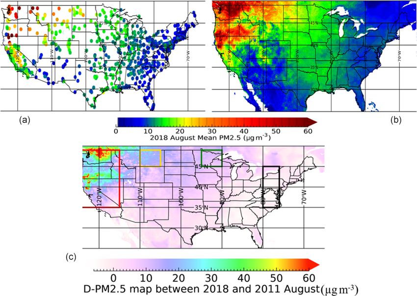
11244                                       Z. Xue et al.: Satellite-based estimation of the impacts of summertime wildfires

2018). According to a recent study, a 10 µg m−3 increase in           The relationship among PM2.5 , AOD and other meteoro-
PM2.5 is associated with a 12.4 % increase in cardiovascu-         logical variables is not spatially consistent (Hoff and Christo-
lar mortality (Kollanus et al., 2016). In addition, exposure to    pher, 2009; Hu, 2009). Therefore, methods that consider spa-
wildfire smoke is also related to massive economic costs due       tial variability can replicate surface PM2.5 with higher accu-
to premature mortality, loss of workforce productivity, im-        racy. One such method is the GWR, which is a non-stationary
pacts on the quality of life and compromised water quality         technique that models spatially varying relationships by as-
(Meixner and Wohlgemuth, 2004).                                    suming that the coefficients in the model are functions of lo-
   Surface PM2.5 is one of the most commonly used param-           cations (Brunsdon et al., 1996; Fotheringham et al., 1998,
eters to assess the health effects of ambient air pollution.       2003). In 2009, satellite-retrieved AOD was introduced in the
Given the sparsity of measurements in many parts of the            GWR method to predict surface PM2.5 (Hu, 2009), followed
world, it is not possible to use interpolation techniques be-      by the use of meteorological parameters and land use infor-
tween monitors to provide PM2.5 estimates on a square kilo-        mation (Hu et al., 2013). Meteorological variables are crucial
meter basis. Since surface monitors are limited, satellite data    for simulating surface PM2.5 since they interact with PM2.5
have been used with numerous ancillary datasets to estimate        through different processes (Chen et al., 2020), which will be
surface PM2.5 at various spatial scales. Several techniques        discussed in detail in the data section. Several studies (Guo et
have been developed to estimate surface PM2.5 using satel-         al., 2021; Ma et al., 2014; You et al., 2016a) successfully ap-
lite observations from regional to global scales, including        plied the GWR model in estimating PM2.5 in China by using
simple linear regression, multiple linear regression, mixed-       AOD and meteorological features as predictors. Similarly to
effect models, chemical transport models (scaling methods),        all the statistical methods, however, the GWR relies on an
geographically weighted regression (GWR), and machine-             adequate number and density of surface measurements (Chu
learning methods (see Hoff and Christopher, 2009, for a re-        et al., 2016; Gu, 2019; Guo et al., 2021), underscoring the
view). The commonly used global satellite data product is          importance of adequate ground monitoring of surface PM2.5 .
the 550 nm (mid-visible) aerosol optical depth (AOD), which           In this paper, we use satellite data from the Moderate Res-
is a unitless columnar measure of aerosol extinction. Simple       olution Imaging Spectroradiometer (MODIS) and surface
linear regression methods use satellite AOD as the only in-        PM2.5 data combined with meteorological and other ancillary
dependent variable, which shows limited predictability com-        information to develop and use the GWR method to estimate
pared to other methods, and correlation coefficients vary          PM2.5 . The use of the GWR method is not novel, and we
from 0.2 to 0.6 from the western to eastern United States          merely use a proven method to estimate surface PM2.5 from
(Zhang et al., 2009). Multiple linear regression methods use       forest fires. We calculate the change in PM2.5 between high
numerous variables along with AOD data, and the predic-            fire activity (2018) and low fire activity (2011) periods dur-
tion accuracy varies with different conditions, including the      ing summer to assess the role of NWUSC wildfires in surface
height of the boundary layer and other meteorological condi-       PM2.5 in the United States. The paper is organized as follows.
tions (Goldberg et al., 2019; Gupta and Christopher, 2009b;        We describe the datasets used in this study, followed by the
Liu et al., 2005). For both univariate and multi-variate mod-      GWR method. We then describe the results and discussion,
els, the AOD shows stronger correlation with PM2.5 dur-            followed by a summary with conclusions.
ing fire episodes compared to pre-fire and post-fire periods
(Mirzaei et al., 2018). Chemistry transport models (CTMs)
that scale the satellite AOD by the ratio of PM2.5 to AOD          2     Data
simulated by models can provide PM2.5 estimations without
ground measurements, which are different from other statis-        A 17 d period (9 to 25 August) in 2018 (high fire activity)
tical methods (Van Donkelaar et al., 2006, 2019). However,         and 2011 (low fire activity) was selected based on analysis
the CTM models depend on reliable emission data, show lim-         of total fires (details in the methodology section) to assess
ited predictability at shorter timescales and are largely useful   surface PM2.5 (Table 1).
for studies that require annual averages (Hystad et al., 2012).
Different machine-learning methods, including neuron net-          2.1    Ground-level PM2.5 observations
works, random forests, and deep belief networks, show im-
provements in prediction accuracy (with CV R 2 values larger       Daily surface PM2.5 from the Environmental Protection
than 0.8), which is hard to accomplish for other parametric        Agency (EPA) is used in this study. These data are from Fed-
regression models (Gupta and Christopher, 2009a; Hu et al.,        eral Reference Methods (FRM), Federal Equivalent Methods
2017; Li et al., 2017; Wei et al., 2019, 2020, 2021). How-         (FEM), or other methods that are to be used in the National
ever, these methods also require a large number of samples         Ambient Air Quality Standards (NAAQS) decisions. A to-
to train the model, which means it is more suitable for daily      tal of 1003 monitoring sites in the US are included in our
PM2.5 estimation rather than short-term wildfire events with       study, with 949 having valid observations in the study period
relatively low occurrence frequency.                               in 2018 and a total of 873 sites with 820 having valid obser-
                                                                   vations in the study period in 2011. PM2.5 values less than

Atmos. Chem. Phys., 21, 11243–11256, 2021                                          https://doi.org/10.5194/acp-21-11243-2021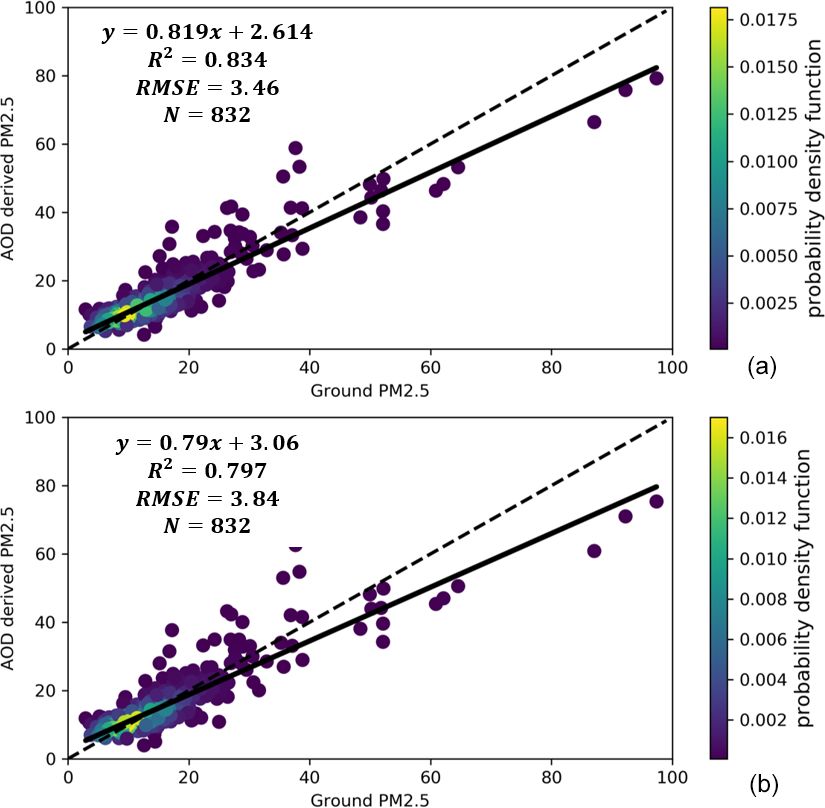
Z. Xue et al.: Satellite-based estimation of the impacts of summertime wildfires                                                                                                11245

Table 1. Datasets used in the study with sources.

              Data/model                                               Sensor                         Spatial          Temporal         Accuracy
                                                                                                      resolution       resolution
        1     Surface PM2.5                                            TEOM                           Point data       Daily            ±5 %–10 %
        2     Mid-visible aerosol optical depth (AOD)                  MAIAC_MODIS                    1 km             Daily            66 % compared to AERONET
        3     Fire radiative power (FRP)                               Terra/Aqua-MODIS               1 km             Daily            ±7 %
        4     ECMWF (meteorological variables)                                                        0.25◦            Hourly

      https://www.epa.gov/outdoor-air-quality-data, https://earthdata.nasa.gov/, https://earthdata.nasa.gov/, https://www.ecmwf.int/en/forecasts (last access: 26 July 2021).

2 µg m−3 are discarded since they are lower than the estab-                                    Aqua fire products to assess wildfire activity. The fire radia-
lished lower detection limit (LDL) (EPA, 2011, 2018).                                          tive energy indicates the rate of combustion, and thus FRP
                                                                                               can be used for characterizing active fires (Freeborn et al.,
2.2      Satellite data                                                                        2014). For the purposes of the study we sum the FRP within
                                                                                               every 2.3◦ × 3.5◦ box to represent the total fire activity in
AOD, which represents the total column aerosol mass load-                                      different locations.
ing, is related to surface PM2.5 as a function of aerosol prop-
erties (Koelemeijer et al., 2006):
                                                                                               2.3     Meteorological data
                     3Qext,dry
AOD = PM2.5 H f (RH)           = PM2.5 H S,                                         (1)
                      4ρ reff                                                                  Meteorological information, including boundary layer height
where H is the aerosol layer height, f (RH) is the ratio of am-                                (BLH), 2 m temperature (T2M), 10 m wind speed (WS),
bient and dry extinction coefficients, Qext,dry is the extinction                              surface relative humidity (RH) and surface pressure (SP),
efficiency under dry conditions, reff is the particle effective                                is obtained from the European Centre for Medium-Range
radius, ρ is the aerosol mass density and S is the specific                                    Weather Forecasts (ECMWF) reanalysis (ERA5) product,
extinction efficiency (m2 g−1 ) of the aerosol under ambient                                   with a spatial resolution of 0.25◦ and temporal resolution
conditions. Although AOD usually has a positive correlation                                    of 1 h, and is matched temporally with the satellite over-
with PM2.5 , this relationship depends on various meteorolog-                                  pass time. The meteorological parameters provide important
ical parameters which will be discussed in Sect. 2.3.                                          information on different processes affecting surface PM2.5
   The MODIS mid-visible AOD from the Multi-Angle Im-                                          concentration, which can also be seen as supplements of the
plementation of Atmospheric Correction (MAIAC) product                                         AOD–PM2.5 relationship as previously discussed.
(MCD19A2 version 6) is used in this study. We used the                                            The BLH can provide information on aerosol layer height
MAIAC-retrieved Terra and Aqua MODIS AOD product at                                            (H in Eq. 1) as aerosols are often found to be well mixed
1 km spatial resolution (Lyapustin et al., 2018), where dif-                                   within the boundary layer (Gupta and Christopher, 2009b).
ferent orbits are averaged to obtain mean daily values. Since                                  With the same amount of pollution within the boundary layer,
thick smoke plumes generated by wildfires can be misclassi-                                    the higher the BLH, the more PM2.5 is distributed within
fied as clouds, only AOD less than 0 will be discarded. Vali-                                  that layer and vice versa (Miao et al., 2018; Zheng et al.,
dation with AERONET studies shows that 66 % of the MA-                                         2017). Therefore, PM2.5 usually has an anticorrelation with
IAC AOD data agree within ±0.5 to ±0.1 AOD (Lyapustin et                                       BLH. However, for wildfire events, the aerosol layer height is
al., 2018). Largely due to cloud cover, grid cells may have a                                  sometimes higher than the BLH (Haarig et al., 2018), which
limited number of AOD observations within a certain period.                                    leads to lower correlation between AOD and PM2.5 since we
On average, cloud-free AOD data are available about 40 % of                                    use only BLH to present the aerosol layer height. Thus BLH
the time during 9 to 25 August 2018 when fires were active                                     can provide aerosol vertical information in most cases ex-
in the region bounded by 25–50◦ N, 65–125◦ W. A smoke                                          cept for suspended high-layer aerosol caused by fires, which
flag from the same product is used as a predictor in estimat-                                  leads to higher bias of the model for high-layer aerosols
ing surface PM2.5 . The smoke detection is performed using                                     near the fire sources. Surface temperature (T2M) can affect
MODIS red, blue and deep blue bands, and smoke pixels are                                      PM2.5 through convection, evaporation, temperature inver-
separated from dust and clouds based on absorption param-                                      sion and secondary pollutant generation processes (Chen et
eter, size parameter and thermal thresholds (see Lyapustin et                                  al., 2020). The first two processes are negatively related to
al., 2012, 2018, for further discussion). The smoke flag data                                  PM2.5 concentration: (1) higher temperature increases tur-
can provide the percentage of a smoke pixel in each grid,                                      bulence, which accelerates the dispersion of pollution and a
which is related to smoke coverage.                                                            decrease in PM2.5 ; (2) higher temperature increases evapo-
   We also use the MODIS level-3 daily FRP (MCD14ML,                                           ration loss of PM2.5 , including ammonium nitrate and other
fire radiative power) product which combines the Terra and                                     volatile or semi-volatile components (Wang et al., 2017). The

https://doi.org/10.5194/acp-21-11243-2021                                                                          Atmos. Chem. Phys., 21, 11243–11256, 2021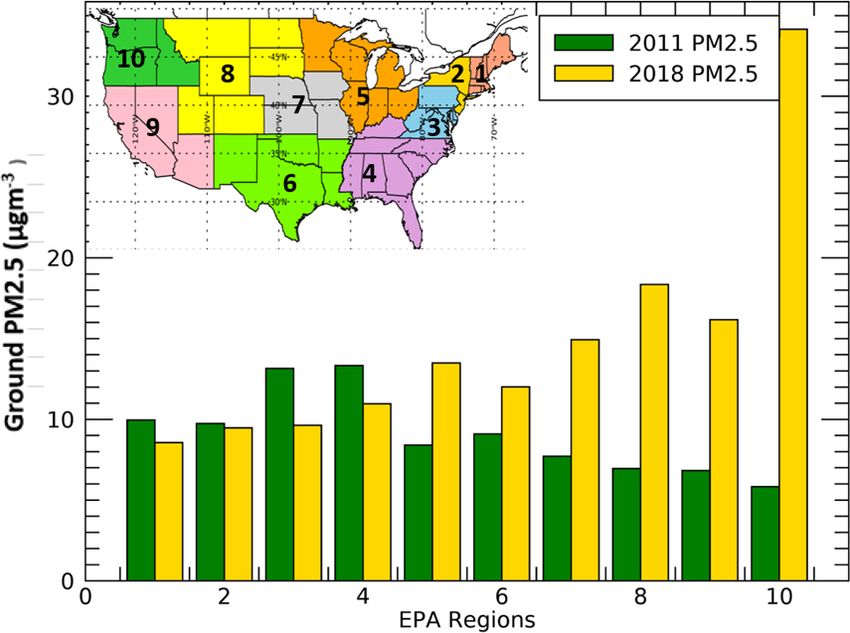
11246                                      Z. Xue et al.: Satellite-based estimation of the impacts of summertime wildfires

latter two processes are positively related to PM2.5 by limit-    ment for some sites and AOD has missing values due to cloud
ing vertical motion and promoting photochemical reactions         cover and other reasons. Therefore, it is important to use data
under high temperature (Xu et al., 2019; Zhang et al., 2015).     from days where both measurements are available to avoid
High wind speeds are often negatively related to PM2.5 since      sampling biases.
it increases the dispersion of pollutants. However, unique ge-
ographical conditions such as mountains with certain wind         3.3    GWR model development and validation
directions can cause accumulation of pollutants (Chen et al.,
2017). RH may promote hygroscopic growth of particles to          The adaptive bandwidth selected by the Akaike information
increase PM2.5 (Trueblood et al., 2018; Zheng et al., 2017).      criterion (AIC) is used for the GWR model (Loader, 1999).
Changes in surface pressure (SP) may influence the diffusion      For locations that already have PM2.5 monitors, we calculate
or accumulation of pollutants through formation of low-level      the mean AOD of a 0.5 × 0.5◦ box centered at the ground lo-
wind convergence (You et al., 2017). Precipitation is another     cation and estimate the GWR coefficients (β) for AOD and
factor that largely influences surface PM2.5 since it can ac-     meteorological variables to estimate PM2.5 . The model struc-
celerate the wash-out of suspended particles, but AOD values      ture can be expressed as
are not available when clouds are present.                        PM2.5i = β0,i + β1,i AODi + β2,i BLHi + β3,i T2Mi
                                                                           + β4,i U10Mi + β5,i RHsf ci + β6,i SPi + β7,i SFi + εi ,
3     Methodology                                                 where PM2.5i (µg m−3 ) is the selected ground-level PM2.5
                                                                  concentration at location i; β0,i is the intercept at location
To assess the impact of NWUSC fires on PM2.5 in the United        i; β1,i ∼ β8,i are the location-specific coefficients; AODi is
States, we first estimate PM2.5 over the study region dur-        the resampled AOD selected from MAIAC daily AOD data
ing a time period with high fire activity (2018). We then use     at location i; BLHi , T2Mi , U10Mi , RHsf ci , and SPi are se-
the same method during a year with low fire activity (2011)       lected meteorological parameters (BLH, T2M, WS, RH, and
to compare the differences between the two years. The two         PS) at location i; SFi (%) is the resampled smoke flag data at
years are selected based on the total FRP in August calcu-        location i, and εi is the error term at location i.
lated within Canada (49–60◦ N, 55–135◦ W) and the north-             We perform leave-one-out cross-validation (LOOCV) to
western (NW) United States (35–49◦ N, 105–125◦ W). Ta-            test the model predictive performance (Kearns and Ron,
ble 2 shows the total FRP in Canada and the northwestern          1999). Since the GWR model relies on an adequate num-
US in August from 2010 to 2018. The total FRP in the two          ber of observations, the prediction accuracy will be lower
regions is lowest in 2011 and highest in 2018 during the          if we preserve too many data for validation. Therefore, we
nine years, which provides the basis for the study. In order      choose the LOOCV method, which preserves only one da-
to create a 0.1◦ surface PM2.5 , the GWR model is used to         tum for validation at a time and repeats the process until all
estimate the relationships of PM2.5 and AOD using various         the data are used. In addition, R 2 and root mean square er-
parameters. Detailed processing steps for the GWR model           ror (RMSE) are calculated for both model fitting and model
are shown in Fig. 1.                                              validation processes to detect overfitting, which leads to low
                                                                  predictability.
3.1    Data preprocessing
                                                                  3.4    Model prediction
The first step is to resample all datasets to a uniform spa-
tial resolution by creating a 0.1◦ resolution grid covering the   While predicting the ground-level PM2.5 for unsampled lo-
continental United States. During this process, we collocate      cations, we make use of the estimated parameters for sites
the PM2.5 data and average the values if there is more than       within a 5◦ radius to generate new slopes for independent
one value in one grid. Then the MAIAC AOD and smoke flag          variables based on the spatial weighting matrix (Brunsdon et
are averaged into 0.1◦ grid cells. Meteorological datasets are    al., 1996). The closer to the predicted location, the closer to
also resampled to the 0.1◦ grid cells by applying the inverse     1 the weighting factor will be, while the weighting factor for
distance method.                                                  sites farther than 5◦ in distance is zero. It is important to note
                                                                  that AOD and other independent variables used for predic-
3.2    Time selecting and averaging                               tion in this step are averaged values for days that have valid
                                                                  AOD, which is different from the data used in the fitting pro-
Next we select data where AOD and ground PM2.5 are both
                                                                  cess since PM2.5 is not measured every day in all locations.
available (AOD > 0 and PM2.5 > 2.0 µg m−3 ) and average
them for the study period (since the LDL for the FRM
method is 2 µg m−3 in 2011 and 3 µg m−3 in 2018, we de-           4     Results and discussion
cided to use the LDL for 2011) (EPA, 2011, 2018). This is
to ensure that the AOD, PM2.5 and other variables match           We first discuss the surface PM2.5 for a few select locations
with each other, because PM2.5 is not a continuous measure-       that are impacted by fires followed by the spatial distribu-

Atmos. Chem. Phys., 21, 11243–11256, 2021                                          https://doi.org/10.5194/acp-21-11243-2021
Z. Xue et al.: Satellite-based estimation of the impacts of summertime wildfires 11247
Figure 1. Flow chart for the geographically weighted regression model used. All satellite, ground, and meteorological data are gridded to 0.1
by 0.1◦ .
Table 2. Total FRP in Canada and the northwestern US in August of different years (unit: 104 MW).
Year 2010 2011 2012 2013 2014 2015 2016 2017 2018
CA 148.24 4.84 19.93 70.54 107.78 10.39 4.6 307.3 542.99
NW US 16.41 42.84 320.39 192.06 67.01 339.58 112.9 195.64 296.91
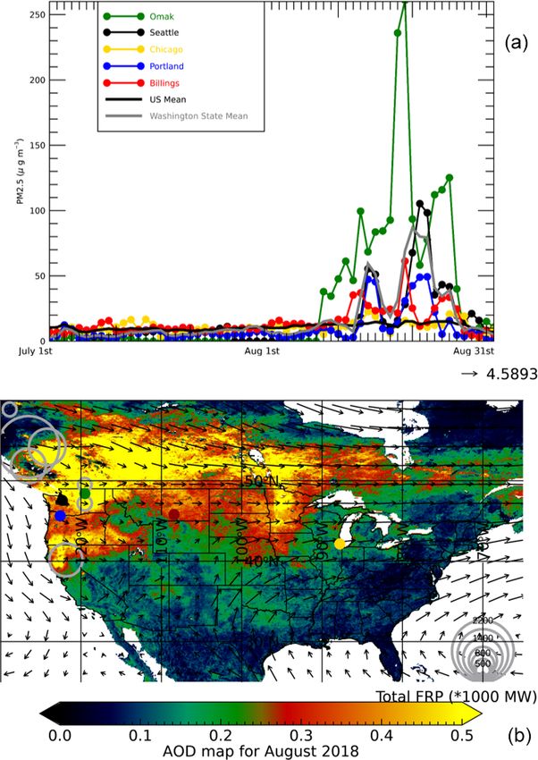
tion of MODIS AOD and the FRP for August 2018. We wildfires in the northwestern US that burnt forest and grass-
then assess the spatial distribution of surface PM2.5 from the land also affected air quality in the United States. Starting
GWR method. The validation of the GWR method is then with the Cougar Creek Fire and then the Crescent Mountain
discussed. To further demonstrate the impact of the NWUSC and Gilbert fires, different wildfires in NWUSC caused se-
fires on PM2.5 air quality in the United States, we show the vere air pollution in numerous US cities. Figure 2a shows
spatial distribution of the difference between August 2018 the rapid increase in PM2.5 in selected US cities from 1 July
and August 2011 and quantify these results for 10 US EPA to 31 August, due to the transport of smoke from these
regions. wildfires. For all sites, July had low PM2.5 concentrations
(< 10 µg m−3 ) and rapidly increases as fire activity increases.
4.1 Descriptive statistics of satellite data and ground Calculating only from the EPA ground observations, the
measurements mean PM2.5 of the 17 d for the entire US is 13.7 µg m−3
and the mean PM2.5 for Washington (WA) is 40.6 µg m−3 ,
The 2018 summertime Canadian wildfires started around which indicates that the PM pollution is concentrated in the
the end of July in British Columbia and continued until northwestern US for these days. This trend is obvious when
mid-September. The fires spread rapidly to the south of comparing the mean PM2.5 of all US stations (black line
Canada during August, causing high concentrations of smoke with no markers) and the mean PM2.5 of all WA stations
aerosols to drift down to the US and affecting particulate mat- (grey line with no markers). Ground-level PM2.5 reaches
ter air quality significantly. From late July to mid-September,
https://doi.org/10.5194/acp-21-11243-2021 Atmos. Chem. Phys., 21, 11243–11256, 202111248 Z. Xue et al.: Satellite-based estimation of the impacts of summertime wildfires
Table 3 shows relevant statistics for 15 states that have
at least one daily record of non-attainment of EPA stan-
dards (> 35 µg m−3 ). From the frequency records of non-
attainment in the 17 d period (last column), four states (Mon-
tana, Washington, California and Idaho) were consistently
affected by the wildfires, and large portions of ground sta-
tions in these states were influenced by smoke aerosols. Most
of the neighboring states also experienced significant air pol-
lution (third column). Noticeable from these records is that
the total number of ground stations in some of the highly af-
fected states (such as Idaho) is not sufficient for capturing
the smoke. Although there are a total of eight EPA stations in
Idaho, only two of them have consistent observations during
the fire event; the other two stations have no valid observa-
tions, and the remaining four stations have only two to six
observations during the 17 d period. Limited availability of
valid data along with unevenly distributed stations makes it
hard to quantify smoke pollution in the northwestern US dur-
ing the fire event period. Therefore, we utilize satellite data to
enlarge the spatial coverage and estimate pollution at a finer
spatial resolution.
The spatial distribution of AOD shown in Fig. 2b indicates
that the smoke from Canada is concentrated mostly in north-
ern US states such as Washington, Oregon, Idaho, Montana,
North Dakota and Minnesota. The black arrow shows the
mean 800 hPa-level mean wind for 17 d, and the length of
the arrow represents the wind speed in m s−1 . Also shown in
Fig. 2b are wind speeds close to the fire sources which are
about 4–5 m s−1 , and according to the distances and wind
Figure 2. (a) Variations of EPA ground-observed PM2.5 in differ-
directions, it can take approximately 28–36 h for the smoke
ent cities from July to August 2018 (Omak – Washington, Seattle – to be transported southeastward to Washington. Then the
Washington, Chicago – Illinois, Portland – Oregon, Billings – Mon- smoke continues to move east to other northern states such
tana). Black line without markers shows the mean variation of all as Montana and North Dakota. In addition, the grey circle
the US stations, and the grey line without markers shows the mean represents the total FRP of every 2.3 × 3.5◦ box. The rea-
variation of stations in Washington State. (b) Mean MAIAC satellite son for not choosing a smaller grid for the FRP is to not
AOD distribution from 9 to 25 August 2018. AOD values equal to clutter Fig. 2b with information from small fires. The big-
or larger than 0.5 are shown as the same color (yellow). Also shown ger the circle is, the stronger the fire is in that grid, and dif-
are circles with FRP. Black arrow shows the wind direction, and the ferent sizes and its corresponding FRP values are shown in
length of it represents the wind speed. The round spots of differ- the lower-right corner. It is clear that the strongest fires in
ent colors on the map show the locations of the five selected cities
2018 are located in Tweedsmuir Provincial Park of British
(green – Omak, black – Seattle, yellow – Chicago, blue – Portland,
red – Billings).
Columbia in Canada (53.333◦ N, 126.417◦ W). The four sep-
arate lightning-caused wildfires burnt nearly 301 549 ha of
the boreal forest. The total FRP of August 2018 in Canada is
about 5362 (· 1000 MW), while the total FRP of August 2011
peak values between 17 and 21 August, and daily PM2.5 val- in Canada is 48 (· 1000 MW). The 2011 fire was relatively
ues during this time period far exceed the 17 d mean PM2.5 . weak compared to the 2018 Tweedsmuir Complex fire, and
For example, mean PM2.5 in Washington on 20 August is we therefore use the 2011 air quality data as a baseline
86.75 µg m−3 , which is more than 2 times the 17 d average to quantify the 2018 fire influence on PM2.5 in the United
of this region. On 19 August, Omak, which is located in the States.
foothills of the Okanogan Highlands in WA, had PM2.5 val-
ues that exceed 250 µg m−3 . According to a review of US 4.2 Model fitting and validation
wildfire-caused PM2.5 exposures, 24 h mean PM2.5 concen-
trations from wildfires ranged from 8.7 to 121 µg m−3 , with The main goal for using the GWR model is to help predict
a 24 h maximum concentration of 1659 µg m−3 (Navarro et the spatial distribution of PM2.5 for places with no ground
al., 2018). monitors while leveraging the increased spatial resolution of
Atmos. Chem. Phys., 21, 11243–11256, 2021 https://doi.org/10.5194/acp-21-11243-2021Z. Xue et al.: Satellite-based estimation of the impacts of summertime wildfires 11249
Table 3. Statistics of 15 states that violate EPA standards (35 µg m−3 ) during the 17 d wildfire period.
State Number of Number of Percentage Number of
sites violating sites in of sites violating days violate
standard the state standard (%) standard
Montana 14 15 93.34 16
Washington 18 20 90 16
Oregon 12 14 85.71 5
North Dakota 7 11 63.63 4
Idaho 5 8 62.5 8
Colorado 11 21 52.38 2
South Dakota 5 10 50 1
California 57 119 47.9 14
Utah 7 15 46.67 4
Nevada 4 13 30.77 1
Wyoming 7 24 29.2 2
Minnesota 4 26 15.4 2
Texas 3 37 8.1 1
Louisiana 1 14 7.1 1
Arizona 1 20 5 1
satellite AOD, and therefore it is important to ensure that the tion error of the model is between 3 and 5 µg m−3 , which
model is robust. Figure 3a and b show the results for 2018 for is a reasonable error range for 17 d average prediction of
GWR model fitting for the entire US and the LOOCV mod- PM2.5 . For data greater than the daily mean EPA standard
els, respectively. The color of the scatter plots represents the (35 µg m−3 ), the model has a RMSE of 12.07 µg m−3 , which
probability density function (PDF) which calculates the rel- is a lot larger than the RMSE when using the entire model.
ative likelihood that the observed ground-level PM2.5 would Therefore, the model has a tendency to underestimate PM2.5
equal the predicted value. The lighter the color is, the more exceedances by around 12.07 µg m−3 . The larger the PM2.5
points are present, with a higher correlation. The model fit- is, the more the model underestimates. To examine the model
ting process estimates the slope for each variable, and there- performance for high- and low-pollution areas, the results are
fore the model can be fitted close to the observed PM2.5 , and divided into two parts (larger than 35 µg m−3 and less than
using this estimated relationship, we are able to assess sur- 35 µg m−3 ). Areas with high pollution have an R 2 of 0.64
face PM2.5 using other parameters at locations where PM2.5 and areas with low pollution have an R 2 of 0.67; therefore,
monitors are not available. The LOOCV process tests the the model performance is relatively stable for both large and
model performance for predicting PM2.5 . If the results of small PM2.5 values. Also, the inclusion of low aerosol con-
LOOCV have a large bias from the model fitting, then the centration areas does not influence the model performance
predictability of the model is low. Higher R 2 and RMSE dif- for high values (seen in the Supplement in Figs. S1 and S2),
ferences indicate that the model is overfitting and therefore which means that the high R 2 is not a reason for the large
not suitable. The R 2 for the model fitting is 0.834, and the number of low values. The GWR model fitting and valida-
R 2 for the LOOCV is 0.797, while the RMSE for the GWR tion results for the 17 d in 2011 are shown in Fig. S3.
model fitting is 3.46 µg m−3 , and for LOOCV the RMSE is
3.84 µg m−3 . There are minor differences between fitting R 2 4.3 Predictors’ influence during wildfires
and validation R 2 (0.037) and between fitting RMSE and val-
idation RMSE (0.376 µg m−3 ), suggesting that the model is
Table 4 shows the GWR model mean coefficients for the
not overfitting and has stable predictability, further indicating
whole US region and for different selected regions. The se-
that the model can predict surface PM2.5 reliably. In addition,
lected boxes are shown in Fig. 4c in different colors: box1
we also performed a 20-fold cross-validation by splitting the
(red) located in the NW US includes major fire sources in
dataset into 20 consecutive folds, and each fold is used for
the US; box2 (gold) located in Montana is influenced by both
validation, while the 19 remaining folds form the training set.
neighboring states and smoke from Canada; box3 (green) in
The 20-fold cross-validation has an R 2 of 0.745 and a RMSE
Minnesota is located further from the fires and has a mi-
of 4.3 µg m−3 . The increase/decrease in the cross-validated
nor increase in PM2.5 due to remote smoke; box4 (black) in
R 2 and RMSE indicates that sufficient data are used for fit-
the NE (northeastern) US is furthest from the fires and has
ting since a small decrease in the number of fitting data can
no obvious pollution increase. The second column of the ta-
reduce the model prediction accuracy. Overall, the predic-
bles shows the conditions for sample selection, and the third
https://doi.org/10.5194/acp-21-11243-2021 Atmos. Chem. Phys., 21, 11243–11256, 202111250 Z. Xue et al.: Satellite-based estimation of the impacts of summertime wildfires
AOD are important for the prediction. We tested our model
with AOD as the only predictor to conduct a comparison to
the original model, and the R 2 decreases from 0.83 to 0.79
and RMSE increases from 3.46 to 3.8. This is consistent with
a previous study (Jiang et al., 2017) which shows improve-
ments of R 2 from 0.69 to 0.78 and RMSE from 7.25 to 6.18
by adding four meteorological parameters in summer in east-
ern China. Other predictors have higher weighting in the fire
source region (box1), where BLH cannot provide the aerosol
vertical distribution information since smoke tends to be in-
jected to higher levels. For high AOD regions where aerosol
tends to be suspended at high levels, adding predictors other
than AOD tends to have lower improvement of the model
compared to low AOD values, because adding BLH can sig-
nificantly improve the prediction for low-level aerosols. For
regions with AOD less than 35, R 2 increases by 0.09 from
the AOD-only model (0.6 to 0.69), while R 2 increases by
0.05 for areas with AOD larger than 35. RMSE decreases by
12 % and 7 % for AOD less and larger than 35 conditions,
respectively. Overall, the meteorological factors have larger
improvements for low-pollution areas (low-level aerosol in
Figure 3. Results of model fitting and cross-validation for the GWR this case).
model for the entire US region averaged from 9 to 25 August 2018.
(a) GWR model fitting results; (b) GWR model LOOCV results.
4.4 Predicted PM2.5 distribution
The dashed line is the 1 : 1 line as a reference and the black line
shows the regression line. The color of the scatter plots represents
the probability density function which provides a relative likelihood The mean PM2.5 distributions over the United States shown
that the value of the random variable would equal a certain sample. in Fig. 4a are calculated by averaging the surface PM2.5
data from ground monitors for the 17 d, which matches well
with the GWR model-predicted PM2.5 distributions shown in
Fig. 4b. The model estimation extends the ground measure-
column shows the number of pixels selected for each box. ments and provides pollution assessments across the entire
By comparing the coefficients of samples selected in these nation. Comparing the AOD map (Fig. 2b) with the PM2.5
boxes, predictors have different influences in different lo- estimations (Fig. 4b) demonstrates the differences between
cations. AOD has a stronger influence on predicting PM2.5 columnar and surface-level pollution. Differences between
closer to fire sources, but local emissions become more domi- the AOD and PM2.5 distributions are for various reasons, in-
nant if the distances are large enough. The smoke flag is over- cluding (1) areas with high PM2.5 concentrations in Fig. 4b
all positively related to surface PM2.5 , while it could slightly corresponding to low AOD values in Fig. 2b (southern Cali-
negatively relate to PM2.5 around fire sources and the north- fornia, Utah, and the southern US) and (2) and high AOD re-
eastern coasts. PBL is negatively related to PM2.5 when the gions in Fig. 2b corresponding to low PM2.5 concentrations
pollution is concentrated near the surface (fires or human- in Fig. 4b (Minnesota). The first situation usually occurs at
made emissions), while it appears to be positively related to the edge of polluted areas that are relatively far from the
PM2.5 in locations where the main pollution source comes fire source, which is consistent with previous studies that re-
from remote wildfire smoke. Surface temperature has a rel- ported smaller particles (< 10 µg) being able to travel longer
atively stable positive correlation with surface PM2.5 ; how- distances compared to large particles (> 10 µg) (Gillies et
ever, surface pressure and wind speeds are negatively corre- al., 1996) and larger particles tending to settle closer to their
lated with PM2.5 . Relative humidity, on the other hand, shows source (Sapkota et al., 2005; Zhu et al., 2002).
large variations in PM2.5 influence across the nation. Around We use the same method for 9 to 25 August in 2011 that
the wildfires where the RH is relatively low, RH has a pos- had low fire activity, ensuring consistency in estimating co-
itive correlation with PM2.5 since hygroscopicity would in- efficients for different variables for 2011. Figure 4c shows
crease and leads to accumulation of PM2.5 , but increasing the difference in spatial distribution of mean ground PM2.5
RH can also decrease PM2.5 concentration by overgrowing of the 17 d between 2018 and 2011. Larger differences in
the PM2.5 particles to deposition in a high-RH environment PM2.5 are in the northwestern and central parts of the United
(Chen et al., 2018). States, with the southern states having very little impact due
From Table 4, we know that the weighting for AOD is to the fires. Of all 48 states within the study region, there
much larger than other predictors, but predictors other than are 29 states that have a higher PM2.5 value in 2018 than
Atmos. Chem. Phys., 21, 11243–11256, 2021 https://doi.org/10.5194/acp-21-11243-2021Z. Xue et al.: Satellite-based estimation of the impacts of summertime wildfires 11251
Figure 4. (a) EPA ground-observed PM2.5 distribution over the US averaged from 9 to 25 August 2018. (b) GWR-predicted 17 d mean
PM2.5 distribution. (c) Difference map of predicted ground PM2.5 of the 17 d mean values between 2018 and 2011. PM2.5 values equal to or
larger than 60 µg m−3 are shown as the same color (red). Note that the D-PM2.5 has a different color scale to make the negative values more
apparent (blue).
Table 4. Coefficients of different predictors.
Mean coefficients Sample selection N AOD Smoke flag PBL T2M RH U SP
box1 (red) FRP > 1000 213 91.94 −0.14 −2.25 0.33 0.08 −2 −0.06
box2 (gold) PM2.5 > 30 362 60.1 0.013 −2.9 0.23 −0.08 −1.6 −0.03
box3 (green) PM2.5 > 17 278 6.2 0.05 0.2 0.2 0.014 −0.3 −0.02
box4 (black) 17 > PM2.5 > 10 938 7.1 −0.02 −1.2 0.22 −0.035 0.06 −0.005
Whole US region ∼ 106 352 28.1 0.024 −0.9 0.06 −0.04 −0.7 −0.002
2011, and 15 states have a 2018 PM2.5 value of more than 34.2 µg m−3 that is 6 times larger than the values in 2011
2 times their 2011 value (shown in Fig. 5). The mean PM2.5 (5.8 µg m−3 ). The PM2.5 of regions 8 and 9 has 2.4 and 2.6
for WA increases from 5.87 in 2011 to 46.47 µg m−3 in 2018, times increases in 2018 compared to 2011. Regions 1–4 have
which is about 8 times more than 2011 values. The PM2.5 lower PM2.5 in 2018 than 2011, possibly due to Clean Air
values in Oregon increase from 4.97 in 2011 to 33.3 µg m−3 Act initiatives, absence of any major fire activities and being
in 2018, which is nearly a 7-fold increase. For states from further away for transported aerosols. The emission reduc-
Montana to Minnesota, the mean PM2.5 decreases from east tion improves the US air quality and lowers the PM2.5 ev-
to west, which reveals the path of smoke transport. As shown ery year, but 6 out of the 10 EPA regions show significant
in Fig. 4c, there is a clear transport path of smoke from North increases in PM2.5 during the study period, which indicates
Dakota all the way to Texas. Along the path, smoke increases that the long-range transported wildfire smoke has become
PM2.5 concentrations by 168 % in North Dakota and 27 % in the new major pollutant in the US.
Texas. Smoke aerosols transported over long distances typi-
cally contain fine-fraction PM, which significantly affects the 4.5 Estimation of Canadian fire pollution
health of children, adults, and vulnerable groups.
Figure 6 shows the mean PM2.5 predicted from the GWR To evaluate the pollution caused only by Canadian fires,
model of different EPA regions for the 17 d in 2011 and 2018 we did a rough assessment according to the total FRP and
(Hawaii and Alaska are not included). The most influenced PM2.5 values. There are three states in the US that have
region is region 10, which has a 2018 mean PM2.5 value of wildfires during the study period, California, Washington
and Oregon, and they have total FRPs of 1186, 518 and
https://doi.org/10.5194/acp-21-11243-2021 Atmos. Chem. Phys., 21, 11243–11256, 202111252 Z. Xue et al.: Satellite-based estimation of the impacts of summertime wildfires
Figure 5. Mean PM2.5 from 9 to 25 August 2018 and 2011 of most affected states.
ence of Canadian wildfires on US air quality is only a rough
quantity estimation, and thus additional work is needed to un-
derstand long-range transport smoke pollution and its impact
on public health.
4.6 Comparison to previous studies
Compared to the Bayesian ensemble model developed by
Geng et al. (2018) using MAIAC AOD and CMAQ (Com-
munity Multiscale Air Quality) model and ground PM2.5
measurements, our GWR model has larger R 2 , but with the
CTM, their method can provide more vertical distribution
information, which is important for wildfire smoke. GWR
usually has better accuracy than the CTM since there are
large uncertainties related to different CTM inputs such as
emission and meteorological and land cover data, but for re-
Figure 6. Mean PM2.5 of EPA regions from 9 to 25 August 2011 gions with fewer or no ground measurements, the CTM pro-
and 2018. Inset shows the map of 10 EPA regions in different colors. vides a good approach for estimating surface PM2.5 . Other
Yellow column represents the 2018 mean PM2.5 , and green column studies which used machine-learning methods to predict sur-
represents for 2011 mean PM2.5 . face PM2.5 have better performance for long-term prediction
rather than monthly estimations (Liang et al., 2020; Xiao et
al., 2018) but can better resolve complex relationships be-
439 (· 1000 MW), respectively. Assuming that California tween different predictors than statistical models (Geng et al.,
was only influenced by the local fires, then fires of 1186 2020). For wildfire events, the available data are much fewer
(· 1000 MW) cause a 13 µg m−3 increase in PM2.5 . Accord- than the long-term aerosol analysis, so the performance of
ingly, wildfires in Washington State and Oregon State will a machine-learning method could be less accurate compared
cause 6 and 5 µg m−3 increases in state mean PM2.5 . There- to long-term prediction. Our study also shows slightly larger
fore, Canadian fires caused PM2.5 increases in Washington R 2 compared to other GWR studies (Hu et al., 2013; Ma et
and Oregon of about 35 and 23 µg m−3 , respectively. Since al., 2014; You et al., 2016b) due to the inclusion of more me-
the FRP of Canadian wildfires is approximately 5 times teorological and other related predictors.
larger than that of the California fires, which are the strongest
fires in the US, we assume that the pollution affecting the 4.7 Model uncertainties and limitations
states located in the downwind directions other than the three
states is mainly coming from Canadian wildfires. States with There are various sources of uncertainties and limitations for
no local fires such as Montana, North Dakota, South Dakota studies that use satellite data to estimate surface PM2.5 con-
and Minnesota have PM2.5 increases of 18.31, 12.8, 10.4 and centrations. Since wildfires develop quickly, it is important to
10.13 µg m−3 . The decrease in these numbers reveals that the have continuous observations to capture the rapid changes.
smoke is transported in a southeasterly direction. This influ- This study uses polar-orbiting high-quality satellite aerosol
Atmos. Chem. Phys., 21, 11243–11256, 2021 https://doi.org/10.5194/acp-21-11243-2021Z. Xue et al.: Satellite-based estimation of the impacts of summertime wildfires 11253
products, but the temporal evolution can only be estimated by states are Washington, California, Wisconsin, Colorado and
geostationary datasets. Although satellite observations have Oregon, all of which have populations greater than 4 million.
excellent spatial coverage, missing data due to cloud cover According to the Centers for Disease Control and Preven-
are a limitation. As discussed in the paper, the prediction er- tion (CDC), 8 % of the population has asthma (CDC, 2011).
ror (RMSE) of the model is between 3 and 5 µg m−3 , while Therefore, for asthma alone, there are about 3 million people
the RMSE increased for locations with high aerosol concen- facing significant health issues due to the long-range trans-
tration. This is partly due to lack of accurate vertical distribu- port of smoke in these states.
tion information, which is very important for wildfire smoke. For states that show a decrease in PM2.5 due to the Clean
The GWR model is largely influenced by the distribution Air Act, the mean decrease is about 16 % of the baseline
of ground stations, and the prediction error will be differ- after 7 years. This is consistent with the EPA’s report that
ent in different locations due to unevenly distributed PM2.5 there is a 23 % decrease in PM2.5 on national average from
stations. For locations that have a dense ground-monitoring 2010 to 2019 (U.S. Environmental Protection Agency, 2019).
distribution, the prediction error will be low, while the pre- Compared to the dramatic increase (132 %) caused by wild-
diction error will be relatively larger in other places with fires, pollution from the fires counteracts our effort on emis-
sparse surface stations. Although there are obvious limita- sion controls. Although wildfires are often episodic and short
tions, complementing surface data with satellite products and term, high frequency of fire occurrence and increasingly
meteorological and other ancillary information in a statis- longer durations of summertime wildfires in recent years
tical model like the GWR has provided robust results for have made them now a long-term influence on public lives.
estimating surface PM2.5 from wildfires. We also note that Our results show a significant increase in pollution in a short
we did not consider some variables used in other studies, time period in most of the US states due to the NWUSC wild-
such as NDVI, forest cover, vegetation type, industrial den- fires, which affects millions of people. With wildfires becom-
sity, visibility and chemical constituents of smoke particles ing more frequent during recent years, more effort is needed
(Van Donkelaar et al., 2015; Hu et al., 2013; You et al., to predict and warn the public about the long-range trans-
2015; Zou et al., 2016). Visibility mentioned in some stud- ported smoke from wildfires.
ies may improve the model performance, but unlike AOD,
it has limited measurement across the nation, which will re-
strict the applicability of training data. Another uncertainty Code availability. The official Python code for the GWR model
comes from the 2011 wildfires, which we assumed to be zero is available at https://github.com/pysal/mgwr (last access: 26 July
fire events, but there are actually few fire events in EPA re- 2021).
gions 6, 8, 9 and 10, and this will lead to underestimation of
PM2.5 increase due to the 2018 fires in these regions.
One limitation of this study is that analysis based on 17 d Data availability. The MAIAC AOD and FRP data are acces-
sible at https://earthdata.nasa.gov/ (last access: 26 July 2021);
mean values cannot capture daily pollution variations, which
the ECMWF meteorological datasets are accessible at https://
is also very important for pollution estimation during rapidly www.ecmwf.int/en/forecasts (last access: 26 July 2021); the sur-
changing wildfire events. To extend this analysis to daily es- face PM2.5 observations are accessible at https://www.epa.gov/
timation, the cloud contaminations of satellite observations outdoor-air-quality-data (last access: 26 July 2021).
become a major problem. Therefore, future work is needed
using chemistry transport models and other data to fill in the
gaps on missing AOD data due to cloud coverage. Supplement. The supplement related to this article is available on-
line at: https://doi.org/10.5194/acp-21-11243-2021-supplement.
5 Summary and conclusions
Author contributions. The authors confirm contribution to the pa-
We estimate the surface mean PM2.5 for 17 d in August for per as follows: study conception and design were by SC, ZX, and
a high fire activity year (2018) and compare that to a low PG; data collection was by ZX and PG; analysis and interpretation
fire activity year using the geographically weighted regres- of results were by ZX, SC, and PG; draft manuscript preparation
sion (GWR) method to assess the increase in PM2.5 in the was done by ZX, SC, and PG. All the authors reviewed the results
and approved the final version of the manuscript.
United States due to smoke transported from fires. The dif-
ference in PM2.5 between the two years indicates that more
than half of the United States (29 states) is influenced by
Competing interests. The authors declare that they have no conflict
the NWUSC wildfires, and half of the affected states have
of interest.
17 d mean PM2.5 increases larger than 100 % of the base-
line value. The peak PM2.5 during the wildfires can be much
larger than the 17 d average and can affect vulnerable popu-
lations susceptible to air pollution. Some of the most affected
https://doi.org/10.5194/acp-21-11243-2021 Atmos. Chem. Phys., 21, 11243–11256, 202111254 Z. Xue et al.: Satellite-based estimation of the impacts of summertime wildfires
Disclaimer. Publisher’s note: Copernicus Publications remains H.: A review on predicting ground PM2.5 concentration us-
neutral with regard to jurisdictional claims in published maps and ing satellite aerosol optical depth, Atmosphere (Basel), 7, 129,
institutional affiliations. https://doi.org/10.3390/atmos7100129, 2016.
Coogan, S. C. P., Robinne, F. N., Jain, P., and Flannigan, M. D.:
Scientists’ warning on wildfire – a canadian perspective, Can.
Acknowledgements. Pawan Gupta and Sundar Christopher were J. Forest Res., 49, 1015–1023, https://doi.org/10.1139/cjfr-2019-
supported by a NASA grant. MODIS data were acquired from the 0094, 2019.
Goddard DAAC. Sincerest thanks to the MAIAC, MODIS, EPA and Dreessen, J., Sullivan, J., and Delgado, R.: Observations and
ECMWF teams for their datasets that made this research possible. impacts of transported Canadian wildfire smoke on ozone
and aerosol air quality in the Maryland region on June
9–12, 2015, J. Air Waste Manage. Assoc., 66, 842–862,
Financial support. This research has been supported by NASA https://doi.org/10.1080/10962247.2016.1161674, 2016.
(grant no. NNM11AA01A). EPA: Code of Federal Regulations Title 40: Protection of Environ-
ment, 694, available at: https://www.govinfo.gov/app/collection/
cfr/2011/ (last access: 26 July 2021) 2011.
EPA: Code of Federal Regulations Title 40: Protection of Environ-
Review statement. This paper was edited by Zhanqing Li and re-
ment, 694, available at: https://www.govinfo.gov/app/collection/
viewed by four anonymous referees.
cfr/2018/ (last access: 26 July 2021) 2018.
Fotheringham, A. S., Charlton, M. E., and Brunsdon, C.: Geograph-
ically weighted regression: a natural evolution of the expansion
method for spatial data analysis, Environ. Plan. A, 30, 1905–
References 1927, 1998.
Fotheringham, S. A., Brunsdon, C., and Charlton, M.: Geograph-
Apte, J. S., Brauer, M., Cohen, A. J., Ezzati, M., and ically Weighted Regression: The Analysis of Spatially Varying
Pope, C. A.: Ambient PM2.5 Reduces Global and Regional Relationships, 2003.
Life Expectancy, Environ. Sci. Technol. Lett., 5, 546–551, Freeborn, P. H., Wooster, M. J., Roy, D. P., and Cochrane, M. A.:
https://doi.org/10.1021/acs.estlett.8b00360, 2018. Quantification of MODIS fire radiative power (FRP) measure-
Brunsdon, C., Fotheringham, A. S., and Charlton, M. E.: ment uncertainty for use in satellite-based active fire characteri-
Geographically Weighted Regression: A Method for Ex- zation and biomass burning estimation, Geophys. Res. Lett., 41,
ploring Spatial Nonstationarity, Geogr. Anal., 28, 281–298, 1988–1994, https://doi.org/10.1002/2013GL059086, 2014.
https://doi.org/10.1111/j.1538-4632.1996.tb00936.x, 1996. Geng, G., Murray, N. L., Tong, D., Meng, X., Chang, H. H.,
Calkin, D. E., Thompson, M. P., and Finney, M. A.: Negative Liu, Y., Hu, X., and Lee, P.: Satellite-Based Daily PM2.5 Es-
consequences of positive feedbacks in us wildfire management, timates During Fire Seasons in Colorado, 123, 8159–8171,
For. Ecosyst., 2, 1–10, https://doi.org/10.1186/s40663-015-0033- https://doi.org/10.1029/2018JD028573, 2018.
8, 2015. Geng, G., Meng, X., He, K., and Liu, Y.: Random forest models for
Cascio, W. E.: Wildland Fire Smoke and Hu- PM2.5 speciation concentrations using MISR fractional AODs
man Health, Sci. Total Environ., 624, 586–595, Random forest models for PM2.5 speciation concentrations us-
https://doi.org/10.1016/j.scitotenv.2017.12.086, 2018. ing MISR fractional AODs, Environ. Res. Lett., 15, 034056,
CDC: Asthma in the US, CDC Vital Signs, May 2011, Center for https://doi.org/10.1088/1748-9326/ab76df, 2020.
Disease Control and Prevention, available at: https://www.cdc. Goldberg, D. L., Gupta, P., Wang, K., Jena, C., Zhang, Y., Lu, Z.,
gov/vitalsigns/asthma/index.html (last access: 26 July 2021), 1– and Streets, D. G.: Using gap-filled MAIAC AOD and WRF-
4, 2011. Chem to estimate daily PM2.5 concentrations at 1 km resolution
Chen, D., Xie, X., Zhou, Y., Lang, J., Xu, T., Yang, N., Zhao, Y., and in the Eastern United States, Atmos. Environ., 199, 443–452,
Liu, X.: Performance evaluation of the WRF-chem model with https://doi.org/10.1016/j.atmosenv.2018.11.049, 2019.
different physical parameterization schemes during an extremely Gu, Y.: Estimating PM2.5 Concentrations Using 3 km MODIS AOD
high PM2.5 pollution episode in Beijing, Aerosol Air Qual. Res., Products: A Case Study in British Columbia, Canada, University
17, 262–277, https://doi.org/10.4209/aaqr.2015.10.0610, 2017. of Waterloo, 2019.
Chen, Z., Xie, X., Cai, J., Chen, D., Gao, B., He, B., Cheng, N., and Guo, B., Wang, X., Pei, L., Su, Y., Zhang, D., and Wang,
Xu, B.: Understanding meteorological influences on PM2.5 con- Y.: Identifying the spatiotemporal dynamic of PM2.5
centrations across China: a temporal and spatial perspective, At- concentrations at multiple scales using geographically
mos. Chem. Phys., 18, 5343–5358, https://doi.org/10.5194/acp- and temporally weighted regression model across China
18-5343-2018, 2018. during 2015–2018, Sci. Total Environ., 751, 141765,
Chen, Z., Chen, D., Zhao, C., Kwan, M. po, Cai, J., Zhuang, https://doi.org/10.1016/j.scitotenv.2020.141765, 2021.
Y., Zhao, B., Wang, X., Chen, B., Yang, J., Li, R., He, B., Gupta, P. and Christopher, S. A.: Particulate matter air qual-
Gao, B., Wang, K., and Xu, B.: Influence of meteorological ity assessment using integrated surface, satellite, and meteoro-
conditions on PM2.5 concentrations across China: A review logical products: 2. A neural network approach, J. Geophys.
of methodology and mechanism, Environ. Int., 139, 105558, Res.-Atmos., 114, 1–14, https://doi.org/10.1029/2008JD011497,
https://doi.org/10.1016/j.envint.2020.105558, 2020. 2009a.
Chu, Y., Liu, Y., Li, X., Liu, Z., Lu, H., Lu, Y., Mao, Z., Chen,
X., Li, N., Ren, M., Liu, F., Tian, L., Zhu, Z., and Xiang,
Atmos. Chem. Phys., 21, 11243–11256, 2021 https://doi.org/10.5194/acp-21-11243-2021Z. Xue et al.: Satellite-based estimation of the impacts of summertime wildfires 11255 Gupta, P. and Christopher, S. A.: Particulate matter air qual- and particulate matter over Europe, Atmos. Environ., 40, 5304– ity assessment using integrated surface, satellite, and meteo- 5315, https://doi.org/10.1016/j.atmosenv.2006.04.044, 2006. rological products: Multiple regression approach, J. Geophys. Kollanus, V., Tiittanen, P., Niemi, J. V., and Lanki, T.: Ef- Res.-Atmos., 114, 1–13, https://doi.org/10.1029/2008JD011496, fects of long-range transported air pollution from vegeta- 2009b. tion fires on daily mortality and hospital admissions in the Haarig, M., Ansmann, A., Baars, H., Jimenez, C., Veselovskii, Helsinki metropolitan area, Finland, Environ. Res., 151, 351– I., Engelmann, R., and Althausen, D.: Depolarization and 358, https://doi.org/10.1016/j.envres.2016.08.003, 2016. lidar ratios at 355, 532, and 1064 nm and microphysi- Li, T., Shen, H., Yuan, Q., Zhang, X., and Zhang, L.: Es- cal properties of aged tropospheric and stratospheric Cana- timating Ground-Level PM2.5 by Fusing Satellite and dian wildfire smoke, Atmos. Chem. Phys., 18, 11847–11861, Station Observations: A Geo-Intelligent Deep Learn- https://doi.org/10.5194/acp-18-11847-2018, 2018. ing Approach, Geophys. Res. Lett., 44, 11985–11993, Hessburg, P. F., Churchill, D. J., Larson, A. J., Haugo, R. D., Miller, https://doi.org/10.1002/2017GL075710, 2017. C., Spies, T. A., North, M. P., Povak, N. A., Belote, R. T., Single- Liang, F., Xiao, Q., Huang, K., Yang, X., Liu, F., Li, J., and Lu, ton, P. H., Gaines, W. L., Keane, R. E., Aplet, G. H., Stephens, X.: The 17-y spatiotemporal trend of PM2.5 and its mortality S. L., Morgan, P., Bisson, P. A., Rieman, B. E., Salter, R. B., burden in China, P. Natl. Acad. Sci. USA, 117, 25601–25608, and Reeves, G. H.: Restoring fire-prone Inland Pacific land- https://doi.org/10.1073/pnas.1919641117, 2020. scapes: seven core principles, Landscape Ecol., 30, 1805–1835, Liu, Y., Sarnat, J. A., Kilaru, V., Jacob, D. J., and Koutrakis, P.: https://doi.org/10.1007/s10980-015-0218-0, 2015. Estimating ground-level PM2.5 in the eastern United States using Hoff, R. M. and Christopher, S. A.: Remote Sensing of Particulate satellite remote sensing, Environ. Sci. Technol., 39, 3269–3278, Pollution from Space: Have We Reached the Promised Land?, J. https://doi.org/10.1021/es049352m, 2005. Air Waste Manage., 59, 645–675, https://doi.org/10.3155/1047- Loader, C. R.: Bandwith selection:Classical or plug in?, Ann. Stat., 3289.59.6.645, 2009. 27, 415–438, 1999. Hu, X., Waller, L. A., Al-Hamdan, M. Z., Crosson, W. L., Estes, M. Lyapustin, A., Korkin, S., Wang, Y., Quayle, B., and Las- G., Estes, S. M., Quattrochi, D. A., Sarnat, J. A., and Liu, Y.: Es- zlo, I.: Discrimination of biomass burning smoke and clouds timating ground-level PM2.5 concentrations in the southeastern in MAIAC algorithm, Atmos. Chem. Phys., 12, 9679–9686, U.S. using geographically weighted regression, Environ. Res., https://doi.org/10.5194/acp-12-9679-2012, 2012. 121, 1–10, https://doi.org/10.1016/j.envres.2012.11.003, 2013. Lyapustin, A., Wang, Y., Korkin, S., and Huang, D.: MODIS Collec- Hu, X., Belle, J. H., Meng, X., Wildani, A., Waller, L. A., tion 6 MAIAC algorithm, Atmos. Meas. Tech., 11, 5741–5765, Strickland, M. J., and Liu, Y.: Estimating PM2.5 Concen- https://doi.org/10.5194/amt-11-5741-2018, 2018. trations in the Conterminous United States Using the Ran- Ma, Z., Hu, X., Huang, L., Bi, J., and Liu, Y.: Estimating ground- dom Forest Approach, Environ. Sci. Technol., 51, 6936–6944, level PM2.5 in china using satellite remote sensing, Environ. Sci. https://doi.org/10.1021/acs.est.7b01210, 2017. Technol., 48, 7436–7444, https://doi.org/10.1021/es5009399, Hu, Z.: Spatial analysis of MODIS aerosol optical depth, PM2.5 , 2014. and chronic coronary heart disease, Int. J. Health Geogr., 8, 1– Meixner, T. and Wohlgemuth, P.: Wildfire Impacts on Water Qual- 10, https://doi.org/10.1186/1476-072X-8-27, 2009. ity, J. Wildl. Fire, 13, 27–35, 2004. Hubbell, B. J., Crume, R. V., Evarts, D. M., and Cohen, J. M.: Melillo, J. M., Richmond, T., and Yohe, G. W.: Climate Policy Monitor: Regulation and progress under the 1990 Clean Change Impacts in the United States: The third national Air Act Amendments, Rev. Environ. Econ. Pol., 4, 122–138, climate assessment, U.S. Global Change Research Program, https://doi.org/10.1093/reep/rep019, 2010. https://doi.org/10.7930/J0Z31WJ2, 2014. Hystad, P., Demers, P. A., Johnson, K. C., Brook, J., Van Donkelaar, Miao, Y., Liu, S., Guo, J., Huang, S., Yan, Y., and Lou, A., Lamsal, L., Martin, R., and Brauer, M.: Spatiotemporal air M.: Unraveling the relationships between boundary layer pollution exposure assessment for a Canadian population-based height and PM2.5 pollution in China based on four-year ra- lung cancer case-control study, Environ. Heal. A Glob. Access diosonde measurements, Environ. Pollut., 243, 1186–1195, Sci. Source, 11, 1–22, https://doi.org/10.1186/1476-069X-11-22, https://doi.org/10.1016/j.envpol.2018.09.070, 2018. 2012. Miller, D. J., Sun, K., Zondlo, M. A., Kanter, D., Dubovik, O., Wel- Gillies, J. A., Nickling, W. G., and Mctainsh, G. H.: Dust con- ton, E. J., Winker, D. M., and Ginoux, P.: Assessing boreal forest centration s and particle-size characteristics of an intense dust fire smoke aerosol impacts on U.S. air quality: A case study us- haze event: inland delta region, Atmos. Environ., 30, 1081–1090, ing multiple data sets, J. Geophys. Res.-Atmos., 116, D22209, https://doi.org/10.1016/1352-2310(95)00432-7, 1996. https://doi.org/10.1029/2011JD016170, 2011. Jiang, M., Sun, W., Yang, G., and Zhang, D.: Modelling Mirzaei, M., Bertazzon, S., and Couloigner, I.: Modeling Wildfire seasonal GWR of daily PM2.5 with proper auxiliary vari- Smoke Pollution by Integrating Land Use Regression and Re- ables for the Yangtze River Delta, Remote Sens., 9, 1–20, mote Sensing Data: Regional Multi-Temporal Estimates for Pub- https://doi.org/10.3390/rs9040346, 2017. lic Health and Exposure Models, Atmosphere (Basel), 9, 335, Kearns, M. and Ron, D.: Algorithmic stability and sanity-check https://doi.org/10.3390/atmos9090335, 2018. bounds for leave-one-out cross-validation, Neural Comput., Munoz-Alpizar, R., Pavlovic, R., Moran, M. D., Chen, J., Gravel, 11, 1427–1453, https://doi.org/10.1162/089976699300016304, S., Henderson, S. B., Sylvain, M., Racine, J., Duhamel, A., 1999. Gilbert, S., Beaulieu, P., Landry, H., Davignon, D., Cousineau, Koelemeijer, R. B. A., Homan, C. D., and Matthijsen, J.: Compari- S., and Bouchet, V.: Multi-Year (2013–2016) PM2.5 Wildfire son of spatial and temporal variations of aerosol optical thickness Pollution Exposure over North America as Determined from https://doi.org/10.5194/acp-21-11243-2021 Atmos. Chem. Phys., 21, 11243–11256, 2021
You can also read