A Radar Object-Based Examination of Rain System Climatology and Including Climate Variability

A Radar Object-Based Examination of Rain System
Climatology and Including Climate Variability
Hooman Ayat (  h.ayat@student.unsw.edu.au )
 University of New South Wales https://orcid.org/0000-0001-9499-5894
Jason P. Evans
 University of New South Wales
Steven C. Sherwood
 University of New South Wales
Joshua Soderholm
 Australian Bureau of Meteorology

Research Article

Keywords: radar object-based examination, rain system, climatology, climate variability, warming, storms,
intensity, rainfall statistics

Posted Date: August 11th, 2021

DOI: https://doi.org/10.21203/rs.3.rs-783979/v1

License:   This work is licensed under a Creative Commons Attribution 4.0 International License.
Read Full License

A radar object-based examination of rain system
 climatology and including climate variability
Hooman Ayat1, Jason P. Evans1, Steven C. Sherwood1, Joshua Soderholm2

1
 Climate Change Research Centre and ARC Centre of Excellence for Climate Extremes,
University of New South Wales, Sydney, New South Wales, Australia
2
 Science and Innovation Group, Australian Bureau of Meteorology, Melbourne, Victoria,
Australia

Corresponding author: Hooman Ayat (h.ayat@student.unsw.edu.au)

1. Abstract

 We know the climate is warming and this is changing some aspects of storms, but we
have little knowledge of storm characteristics beyond intensity, which limits our understanding
of storms overall. In this study, we apply a cell-tracking algorithm to 20 years of radar data at a
mid-latitude coastal-site (Sydney, Australia), to establish a regional storm climatology. The
results show that extreme storms in terms of translation-speed, size and rainfall intensity usually
occur in the warm season, and are slower and more intense over land between ~10am and ~8pm
(AEST), peaking in the afternoon. Storms are more frequent in the cold season and often initiate
over the ocean and move northward, leading to precipitation mostly over the ocean. Using
clustering algorithms, we have found five storm types with distinct properties, occurring
throughout the year but peaking in different seasons. While overall rainfall statistics don't show
any link to climate modes, links do appear for some storm types using a multivariate approach.
This climatology for a variety of storm characteristics will allow future study of any changes in
these characteristics due to climate change.

 1

1 1. Introduction
 2 Heavy rainfall is a significant threat to life and property in many parts of the world,
 3 especially when it is accompanied by flash floods (Johnson et al. 2016; Allen and Allen 2016).
 4 Many studies have shown the potential for climate change to impact rainfall intensity, but how it
 5 will affect other storm characteristics (size, translation speed, orientation, etc.) remains largely
 6 unexplored. The first step towards exploring the potential future changes is to establish an
 7 observed baseline for a wide variety of storm characteristics.
 8 Climatological studies can help us to better understand storm characteristics and their
 9 (local and remote) drivers in different seasons. Many studies have used gridded datasets (e.g.,
10 global climate models, reanalysis data) to perform climatological studies globally and over
11 specific regions; however, the coarse-resolution of these datasets are often unable to properly
12 capture small scale storms like thunderstorms. Therefore, in order to capture these small scale
13 storms using these datasets, researchers have tried to establish thunderstorm climatologies based
14 on the concept of favourable conditions for thunderstorms, which usually includes a combination
15 of convective available potential energy (CAPE) and vertical wind shear in a region (Ahmed et
16 al. 2019; Brooks et al. 2003; Taszarek et al. 2020; Allen et al. 2011; Groenemeijer et al. 2017).
17 By employing this environmental approach, Allen and Karoly (2014) presented a severe
18 thunderstorm climatology over Australia during 2003–2010, using ERA-Interim reanalysis and
19 reported observation data. They showed that these types of storms are more frequent in
20 December during the afternoon, consistent with the seasonal and diurnal cycle of surface
21 temperature and the maximum availability of heating. Although this approach provides valuable
22 information, environmentally favorable conditions do not necessarily lead to a thunderstorm,
23 causing a misestimation of the thunderstorm frequency. In addition, this approach only provides
24 us with storm frequency and it is unable to provide information on other storm characteristics
25 (Allen and Karoly 2014).
26 Using coarse-resolution datasets, previous authors have tried to investigate the effect of
27 natural climate variability (e.g., El Niño–Southern Oscillation (ENSO), the Indian Ocean Dipole
28 (IOD)) on the rainfall over Australia. Ashok et al. (2003) showed that IOD has significant
29 negative partial correlations with rainfall over the western and southern regions of Australia
30 using an atmospheric general circulation model. Allen and Karoly (2014) employed the ECMWF
31 Interim Re-Analysis (ERA-Interim) data and have found that ENSO has a substantial impact on
32 the spatial distribution of severe thunderstorm environments over the continent. In another
33 reanalysis-based study, Hauser et al. (2020) investigated the winter-spring rainfall variability in
34 southeastern Australia (SEA) during El Niño events by quantifying the contribution of clustered
35 mid-latitude weather systems to monthly precipitation anomalies. The authors found that the
36 cluster with below-average rainfall is more frequent compared to the other clusters during El
37 Niño, which confirmed the general suppression of SEA rainfall during these events. Since
38 precipitation in some regions is correlated with more than one large scale driver, and indices are
39 often correlated with each other, the interconnected nature of precipitation dependence suggests

 2

40 the need for a multivariate rather than bivariate approach to this problem. Maher and Sherwood
41 (2014) applied a multivariate approach to Australian precipitation to disentangle the multiple
42 sources of large-scale variability using the ERA-Interim and Australian Water Availability
43 Project datasets, and they showed that ENSO, blocking, and the intensity and position of the
44 ridge are driving wintertime precipitation in Australia, with a minor role played by the jet
45 intensity and the IOD. All of these studies investigated the effects of natural climate variability
46 on rainfall intensity and frequency, and the relationships between other characteristics of storms
47 (i.e., size, shape, translation speed, etc.) and climate modes are not understood.
48 One way of studying the thunderstorm climatology is by measuring the occurrence of
49 lightning using satellite instruments such as the Optical Transient Detector (OTD) and/or the
50 Lightning Imaging Sensor (LIS). Dowdy and Kuleshov (2014) produced a climatological map of
51 lightning ground flash density over Australia, which details the seasonal variability of the
52 lightning ground flash densities over land and ocean. They found that during the cooler months,
53 a maximum in lightning activity occurs over the ocean to the east of the continent. Earlier studies
54 by Kuleshov et al. (2001; 2012) had found that the second-highest thunderstorm frequency
55 occurs in the southeast part of Australia along the coastline, most often from spring to early
56 autumn. Similar research has been conducted globally for regions such as the United States and
57 Europe (Taszarek et al. 2020), Brazil (Pinto et al. 2013) and middle-east (Shwehdi 2005). A
58 limitation of this approach is that it is unable to capture storms without lightning. Additionally, it
59 is only able to provide information regarding storm frequency, not other information like rainfall
60 intensity (Walsh et al. 2016).
61 Rain gauge data and reports of hail, tornado and wind gusts are other means of studying
62 thunderstorm climatology used in many studies (Bhardwaj and Singh 2018; Enno et al. 2013;
63 Saha and Quadir 2016; Pinto et al. 2013; Groenemeijer et al. 2017; Kelly et al. 1985; Doswell et
64 al. 2005). The databases of reported tornadoes, hailstorms, and gust winds in some countries like
65 Australia have a long-term record (Bureau of Meteorology 2021), which can provide valuable
66 information for climatological studies. Using these datasets over Australia, some researchers
67 have found that severe thunderstorms are most prevalent between October and April (Niall and
68 Walsh 2005; Schuster et al. 2005; Davis and Walsh 2008) with a peak between 3 and 7 pm
69 (Griffiths et al. 1993; Schuster et al. 2005), consistent with the findings of Allen and Karoly
70 (2014) using environmental approach and ERA-Interim reanalysis data. Higher frequency of
71 heavy rain events over Australia in summer was also reported by Dare and Davidson (2015),
72 using a high resolution gridded daily rain gauge data. Some efforts have also been made to
73 employ these types of data to investigate relationships between ENSO and storm events, globally
74 (Cook and Schaefer 2008; Cook et al. 2017; Lee et al. 2016, 2013; Lepore et al. 2017) and over
75 Australia (Chung and Power 2017; Risbey et al. 2009a,b; Murphy and Timbal 2008; Nicholls et
76 al. 1996; McBride and Nicholls 1983; Allan et al. 1996; Schepen et al. 2012; Min et al. 2013;
77 King et al. 2014; Ashcroft et al. 2019). Based on these studies, winter-spring rainfall is usually
78 reduced during El Niño and enhanced during La Niña over the eastern and southeastern parts of
79 Australia. Although gauge and reported data provide us with valuable information, the

 3

80 distribution of recorded data is highly influenced by the local population (Allen 2018). In
 81 addition, gauge instruments are point measurements and sparse rain gauge networks often fail to
 82 observe the maximum rainfall (Ayat et al. 2018).
 83 The limitations of previous approaches have led to the application of remotely-sensed
 84 datasets, which are a growing area of thunderstorm climatology. Some studies (Cecil and
 85 Blankenship 2012; Ni et al. 2017) have applied a satellite-based approach using passive and
 86 active microwave sensors to estimate the global climatology of hail storms. However, images
 87 from these sensors are available only for a few overpasses per day (Ayat et al. 2021a), which
 88 may result in biasing the results depending on the diurnal cycle of convection in the respective
 89 regions (Punge and Kunz 2016). In addition, passive microwave products are capturing the upper
 90 part of the storms in which there might be more hail particles that melt/evaporate at lower
 91 altitudes, leading to false estimation of hail on the ground surface (Ayat et al. 2021b).
 92 High spatio-temporal resolution radar rainfall estimates offer the potential to study the
 93 thunderstorms occurring over their coverage areas, particularly over the regions in which gauge
 94 observations are usually sparse or unevenly distributed (Ghaemi et al. 2017; Ayat et al. 2018;
 95 Moazami et al. 2014). Radar records in many parts of the globe are temporally limited to just
 96 over a decade (Allen 2018). However, this time frame is long enough to conduct climatological
 97 studies. Previous researchers have employed these datasets to conduct thunderstorm climatology
 98 studies over specific regions such as the United States (Ghebreyesus and Sharif 2020; Kuo and
 99 Orville 1973; Croft and Shulman 1989; Falconer 1984), Europe (Kaltenboeck and Steinheimer
100 2015; Kreklow et al. 2020; Weckwerth et al. 2011; Overeem et al. 2009; Bližňák et al. 2018;
101 Fairman Jr et al. 2015) and Asia (Chen et al. 2012).
102 Hail particles are readily detected by conventional weather radars due to strong scatter
103 produced by their comparatively larger surface area, or via their quasi-spherical shape which
104 produces distinct differential reflectivity values for dual-polarization radars compared to oblate
105 rain droplets. Using these properties, a few radar-based hail products have been produced and
106 employed to study the climatology of hailstorms over different regions. For instance, Warren et.
107 al (2020) studied the hail climatology in multiple cities in Australia (including the Sydney
108 region) using a radar-based hail product (Maximum Expected Size of Hail; MESH), and found
109 that, on average, damaging hail storms over Sydney occur 32 days per year with a peak during
110 the warm season (November-March). Similar radar-based studies have been conducted over
111 other parts of the globe like Europe (Junghänel et al. 2016; Nisi et al. 2016; Fluck et al. 2021;
112 Lukach et al. 2017; Saltikoff et al. 2010) and the United States (Cintineo et al. 2012; Murillo et
113 al. 2021).
114 Most of the previous radar-based studies employed a pixel-based statistical approach
115 which limits the storm properties to rainfall/hail frequency and intensity as a function of position.
116 In order to overcome this limitation, a few studies have employed an object-based approach,
117 where discrete storm objects are identified and characterized. For instance, Haberlie and Ashley
118 (2019), Poujol et al. (2020) and Prein et al. (2017) applied object-based techniques to radar
119 products to study the climatology of convective storms in the United States. In Australia,

 4

120 Soderholm et al. (2017) employed a cell-tracking algorithm over radar MESH product to study
121 hail climatology in southeast Queensland, Similar efforts have been made in Germany
122 (Thomassen et al. 2020), Italy (Sangiorgio and Barindelli 2020) and Spain (Rigo et al. 2010).
123 Although object-based techniques can provide us with more information on storm
124 characteristics, the investigated storm properties in most of these studies were limited to storm
125 number, area, and rainfall intensity, whereas other storm characteristics like storm translation
126 speed, shape and aspect ratio, orientation, direction and volume could also be of interest. In
127 addition, the object-based techniques employed in these studies are limited by the object
128 split/merge issue, which is a common problem in object tracking methods and can lead to
129 calculating misleading storm properties (Muñoz et al. 2018).
130 In this research, we employ the Method of Object-based Diagnostic Evaluation (MODE)
131 Time Domain (MTD), which is modified by the authors so as to handle splitting and merging of
132 objects. We apply this to the Wollongong (near Sydney) radar, which has around 20 years of
133 records, to establish an object-based climatology of precipitation in different seasons over the
134 radar footprint areas (i.e., Greater Sydney, Illawarra and other land/ocean regions within 150 km
135 of the radar). An effort has been made to group the main contributing storms with similar object-
136 based characteristics over this region using clustering algorithms followed by investigating their
137 relationships with different climate modes.
138 This study is presented in seven sections. Section 2 describes the Wollongong radar data
139 and its characteristics. Section 3 introduces the object-based and clustering methods along with
140 the statistics employed in this study. Section 4 describes the study area and section 5 presents the
141 results of the object-based climatology over the study area. Section 6 discusses the results shown
142 in the previous section, and finally, the summary of findings is presented in section 7.

143 2. Dataset

144 3.1 Radar Data
145 This study uses data from a Bureau of Meteorology operational S-band weather radar
146 located near Wollongong, NSW (34.26° S, 150.87° E, 471 m altitude; (Soderholm et al. 2020)).
147 The site experiences partial blocking up to 3 dB in the lowest scan (0.5° elevation) from the
148 northwest to the southeast due to the significant terrain associated with the Great Dividing
149 Range. The archive for this radar started in November 1996 and continues to operate as of 2021.
150 However, the study period is limited to June 2018 in this study. Several hardware and
151 configuration changes have taken place over the last 24 years. Initially, the radar operated on a
152 10-minute volume cycle with 16-level reflectivity data. In December 1999 the number of
153 reflectivity levels was increased to 64. Between October 2010 and January 2021, a major
154 hardware upgrade delivered 160-level reflectivity data and a 6-minute volume cycle. One
155 significant gap is present in the archive from 1/1/1998 to 15/12/1998.
156 To ensure the accuracy of reflectivity values across the entire dataset, an absolute
157 calibration technique is applied using precipitation radar measurements from the Tropical

 5

158 Rainfall Measuring Mission (TRMM) and the Global Precipitation Measurement Mission
159 (GPM). Satellite overpasses with precipitation are compared with ground radar measurement
160 using the volume matching technique described by Louf et al. (2019), providing a mean
161 calibration value for every pass. Periods of stable calibration are identified, and the mean
162 absolute calibration value for these periods is applied as an offset to the ground radar data.
163 Removal of non-meteorological echoes from reflectivity datasets is challenging. In addition to
164 the ground clutter filtering performed by the signal processor, the technique described by Gabella
165 et al. (2002) is applied using filters for echo continuity and minimum echo area. Unfortunately,
166 this technique is not suitable for removing anomalous propagation which is commonly observed
167 over the adjacent South Pacific Ocean.
168 Reflectivity data is transformed to rain rates using a fitted Z-R relationship derived from
169 9 years of hourly rain gauge data using the Camden Airport AWS (35.04° S, 150.69° E). The A
170 and B coefficients for this relationship were 81 and 1.8 respectively. The maximum rainrate is
171 limited to 100 mm/hr to limit contamination from hail. Volumetric rain rates are transformed into
172 a Cartesian grid at a 0.5 km altitude using the Barnes weighting function and a 2.5km constant
173 radius of influence. The final grid has a horizontal resolution of 1 km and a domain size of 300
174 km by 300 km.

175 3.2 Challenges with anomalous propagation
176 Despite all the efforts made in removing non-meteorological echoes, the Wollongong
177 radar site experiences significant anomalous propagation over the ocean within the eastern
178 portion of its coverage. These echoes primarily occur during heat-wave conditions, where strong
179 low-level vertical gradients of humidity and temperature create regions of super refraction for
180 lower elevation scans. The resultant echoes have similar reflectivity gradients, size and shape as
181 precipitation echoes, while also being non-stationary, limiting the effectiveness of any
182 algorithms to remove non-meteorological echoes from reflectivity data (fig S5a; Online
183 Resource 1). In order to reduce the effect of these clutter sources in precipitation estimates, we
184 have opted for a two-step clutter removal process over the whole dataset: 1) Since these clutters
185 often include pixels with low intensity, applying the 3 mm/hr threshold over the convolved data
186 (to detect the storm objects; see section 5.1), effectively removed this clutter throughout the year
187 (fig S5b; Online Resource 1) except some extremes in summer (fig S5d; Online Resource 1). 2)
188 The days with extreme clutter were removed manually from the dataset using maximum daily
189 reflectivity maps (see fig S4; Online Resource 1) such that the days with high values of
190 maximum reflectivity over the ocean and low values over land were considered as a day with
191 extreme clutter over the ocean.

192 3. Study area
193 Thestudy area in this research is the radar coverage regions located up to 150 km from
194 the Wollongong radar, which includes coastal regions of Greater Sydney and Illawarra in New

 6

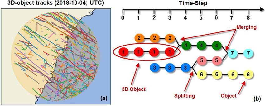
195 South Wales. The climate of these regions is categorized as humid subtropical, or Cfa based on
196 the Köppen–Geiger classification (Kottek et al. 2006), and is significantly affected by the coastal
197 position, with small interseasonal variations ranging from cool winters to warm and hot summers
198 (Bureau of Meteorology 2016; Dare and Davidson 2015). The mean annual precipitation
199 recorded at Observatory Hill (in Greater Sydney) and Wollongong University (in Illawarra)
200 locations are 1213.4 mm and 1348.6 mm, respectively (Bureau of Meteorology 2013).
201 Several factors may impact the precipitation over these regions and its seasonality.
202 Generally, precipitation peaks in the first half of the year and decreases in the second half
203 (Bureau of Meteorology 2013). In the summer, the easterly (or inland) trough is a major
204 contributor to rainfall over these regions with a peak in the evening. Its impact can be enhanced
205 by interacting with any upper-level troughs or cold fronts crossing over these regions. Frontal
206 systems also bring rainfall to these regions throughout the year, but mostly in winter when the
207 subtropical ridge moves northward over inland Australia (Bureau of Meteorology 2010). Another
208 source of precipitation over these regions is cut-off lows, which can occur at any time of year but
209 are most common during autumn and winter. These can be intense and last up to a week when
210 formed as part of a blocking pair or east coast lows, in which case they are accompanied by long-
211 lasting heavy rainfall and gusty winds (Bureau of Meteorology 2007). Northwest cloud bands
212 (stretching from northwest to southeast Australia) can also bring precipitation over these regions.
213 They may interact with cold fronts and cut-off lows over southeastern Australia to produce very
214 heavy rainfall over these regions (Reid et al. 2019). Several modes of variability are known to
215 affect precipitation in Australia, However, precipitation over the coastal zone that includes our
216 study area has shown little relationship (Timbal and Hendon 2011; Fita et al. 2017) Method

217 4.1. Method of Object-based Diagnostic Evaluation (MODE) Time Domain (MTD):
218
219 MTD is an extension for MODE to track the storm objects detected in a precipitation map
220 by the MODE algorithm (Clark et al. 2014). Here we employed a modified version of MTD,
221 proposed by Ayat et al. (2021b), that considers split/merge events during the lifetime of a storm.
222 In this method, the “storm objects” at each time step are the connected pixels higher than a
223 specified threshold in the convolved precipitation map (smoothed by an “n⨯n-pixel” moving
224 window across the map). Every “storm object” at each time-step has a unique label number
225 unless it has overlap with another storm object at the previous time-step (each blob in figure 1b).
226 In this case, it takes the label of the storm object at the previous time-step. If a storm-object has
227 overlap with two (or more) storm objects in the previous time step (merging) or two (or more)
228 objects have overlaps with a storm-object at the previous time step (splitting), the storm-
229 object/storm-objects at the current timestep takes/take a new label. Based on these definitions, A
230 “sequence of objects (or 3D objects)” is the connected storm objects in time that has a unique
231 label number and doesn’t have split/merge events during its lifetime (connected blobs with the
232 same colours and numbers in figure 1b). Finally, a “storm” is a group of the 3D objects that are
233 connected via split/merging events (The whole diagram in figure 1b).

 7

234 Figure 1a represents an example of running the modified MTD on Wollongong radar data
235 during an event that occurred on 2018-10-4. The lines with different colors are showing the 3D-
236 object tracks. In this event, land-originating storms’ parts had a southeastward direction and later
237 were merged with the storms’ parts that had formed over the ocean. Considering split/merge
238 events in this event has shown how successfully this approach could separate storms’ parts over
239 land and ocean before merging which is not possible using the original version of MTD. In
240 addition, with the help of the new approach in tracking the storms, it’s possible to extract storm
241 characteristics with more details from different parts of the storms and better calculate
242 characteristics like translation speed, direction and track length during the lifetime of the storms
243 with high rate of split/merge events.
244 In this research, we are studying the extracted characteristics related to “storms” and
245 “storm objects” using the modified MTD method. The selected threshold to filter the objects is 3
246 mm/hr in the convolved data smoothed by a “3×3-pixel” moving window across the map. The
247 storm-object characteristics of interest in this study include: 1) area: the number of pixels in the
248 storm object; 2) translation speed: the ratio of the distance between the volumetric centroid of
249 two connected objects in time to the temporal resolution of the dataset; 3) maximum intensity:
250 the maximum precipitation rate within a storm object; 4) object average intensity: the average
251 precipitation rate of all cells within a storm object; 5) object volume discharge: the volumetric
252 rain rate that passes through the storm object area during a specified period; 6) aspect ratio: the
253 ratio of the minor and major axis of the fitted ellipse over the storm object; 7) object direction:
254 the compass direction of the line connecting the centroids of two consecutive objects in a
255 sequence, and finally, 8) orientation that is the compass direction of the major axis of the fitted
256 ellipse.
257 The studied storm characteristics in this research include: 1) storm area: the average
258 storm snapshot areas in the storm lifetime; 2) storm volume discharge: the average storm
259 snapshot volume discharge in the storm lifetime; 3) storm average intensity: the average of
260 precipitation rate in the storm lifetime; 4) storm max average intensity: the maximum of storm
261 averaged intensity (calculated at each snapshot) in the storm lifetime; 5) storm translation speed:
262 the area-weighted average translation speed of the storm snapshots in the storm lifetime; 6) storm
263 direction: the area-weighted average direction of the storm snapshots in the storm lifetime; 7)
264 storm contributing objects: The number of root storm objects in the storm graph diagram (e.g. in
265 figure 1 storm object numbers 1, 2 and 3 are the root objects in the storm diagram) and 8) storm
266 split/merge event number: the number of split/merge events in the storm lifetime. Note that no
267 thresholds have been applied over the defined storm/storm-object properties in this study.
268

 8

269
270 Fig. 1 Panel (a) shows the 3D-object tracks for storms that occurred on (2018-10-04;
271 UTC). Panel (b) illustrates the diagram of a tracked storm with split/merge events. Note that each
272 blob represents a storm object at each time step and each colour shows a sequence (or 3D)
273 object.

274 4.2. Clustering Analysis
275 The aim of this section is to find storm clusters (types) with similar quantitative
276 characteristics over the study area using both the Agglomerative clustering algorithm and the t-
277 SNE technique.

278 4.2.1 t-Distributed Stochastic Neighbor Embedding (t-SNE)
279
280 t-SNE is a statistical technique to visualize high-dimensional data by projecting it on a
281 two or three-dimensional map. Here is a brief overview of the main stages in this method: 1) It
282 starts with constructing a probability distribution of similarities over pairs of events in high-
283 dimensional data such that a similar pair of events have a higher value compared to the one that
284 is less similar; then, 2) another probability distribution of similarities is defined over the points in
285 the low-dimensional map, and finally, 3) the algorithm minimizes the divergence between two
286 distributions using Kullback–Leibler divergence parameter (KL divergence) between the two
287 distributions with respect to the locations of the points in the map. Note that the KL divergence
288 parameter is a measure of how one probability distribution diverges from another using a
289 gradient descent method. For more details, please refer to the original research paper by Maaten
290 and Hinton (2008).

291 4.2.2 Agglomerative clustering
292
293 The agglomerative technique is one of the common types of hierarchical clustering in
294 grouping data based on their similarity. This technique works in a “bottom-up” manner by
295 treating each object as a separate group in the beginning. Next, at each step, the two clusters with

 9

296 the most similarity are merged into a bigger cluster and this process continues until all objects
297 are merged into one single big cluster (Subasi 2020). Here we have used the t-SNE algorithm to
298 project our n-dimensional data on a two-dimension map (see fig 9a) and increase the divergence
299 of potential clusters. Then, the agglomerative technique has been employed over the projected
300 data to find the clusters. Similar process has been repeated by applying KMeans clustering
301 algorithm (see fig S3; Online Resource 1). However, based on the density map, the cluster
302 borders have been better recognized by the agglomerative technique.
303 In order to find independent properties as the input for the clustering algorithm, the
304 correlations between all pairs of the storm-object properties have been calculated and the pairs
305 with correlation higher than 0.5 are considered as dependent variables and haven’t been used
306 together as the input in the clustering algorithm. Note that all input data are normalized (ranging
307 from 0-1) by dividing each input storm property by its maximum and standard deviation.
308 One of the problems with hierarchical clustering is that it doesn’t give information
309 regarding the number of clusters, or where to stop the merging process in the algorithm. In order
310 to overcome this limitation, we have employed the Calinski Harabasz index (CHI) to define the
311 number of clusters which is the optimum value of CHI by increasing the number of clusters.
312 CHI is the ratio of between-cluster variance (VARB) to within-cluster variance (VARW):
313
 − 
314 = × (1)
 −1
315 = ∑ 
 =1 | − |
 2
 (2)
 
316 = ∑ 
 =1 ∑ =1 | − |
 2
 (3)
317
318 Here, N is the population of the data, K denotes the number of clusters, and Zk and z refer
319 to the centroid of cluster k and the entire data, respectively. In the second and third equations, n k
320 is the population of cluster k and xi denotes each member of that cluster (Li et al. 2018).

321 4.3. Statistics
322 Here we employed the non-parametric Kendall’s Tau rank correlation coefficient (tau) to
323 investigate the strength of relationships between variables. This value is derived from the
324 following equation:
325
 − 
326 = (4)
 + 
327
328 In this equation, C is the number of matched pairs and D is the number of mismatched
329 pairs of the two variables.
330 To determine the significance of the difference between the two data distributions, the
331 nonparametric statistical Kolmogorov-Smirnov test (KS-test) has been employed. This technique
332 is a non-parametric test which doesn’t need the input data distributions to be normal. The null

 10

333 hypothesis in this test is that both samples come from a population with the same distribution.
334 This null hypothesis is rejected at the level of ⍺ if:
335
 + 
336 , > ( )√ (5)
 × 

337 , = | 1, ( ) − 2. ( )|
338 (6)
 1
339 = √− ( ) × (7)
 2 2
340
341 Where Dn,m denotes the KS statistic and n,m are the sizes of the two datasets. F1, n and
342 F2,m refer to empirical distribution functions for both variables, and sup is the supremum
343 function. Note that the supremum function of a subset S of a set K is the least element in K that
344 is greater than or equal to all elements of S.
345 In order to model the relationship between two or more variables, in this research, we
346 have employed the Ordinary least squares (OLS) method:
347
348 = 
349 (8)
350 = ( )
351 (9)
352 ( ) = ( − ) ( − ) (10)
353
354 Where n is the number of observations, p is the number of independent variables, y is the
355 n×1 matrix of the dependent parameter, X is the n×p matrix of independent variables.
356 Suppose b is a "candidate" value for the parameter β which is the n×1 matrix of
357 coefficients for independent variables.
358 An effort has been made in this study to investigate the relationships between climate
359 indices (i.e., El Niño–Southern Oscillation (ENSO), Indian Ocean Dipole (IOD), and Southern
360 Annular Mode (SAM)) and storm properties in each cluster (derived from the previous section).
361 Since precipitation can be correlated with more than one index, and the indices are often
362 correlated with each other (Maher and Sherwood 2014; Taschetto et al. 2011; Mekanik et al.
363 2013; Mekanik and Imteaz 2012), we have utilized a multivariate approach rather than a
364 bivariate approach to consider the dependency of the climate modes on each other. Equation 11
365 is the model representing the relationship between the three selected indices and each object-
366 based storm properties (in each cluster) for every month using a multiple linear analysis to
367 consider the dependency of the selected indices and include the annual variations.
368
369 . = 0 + 1 × ñ 3.4 + 2 × + 3 × (11)
370

 11

371 Where C0 is the Month constant and C1, C2, C3 are Niño 3.4, IOD and SAM coefficients,
372 respectively. Note that, in this equation, each object-based property at every timestep is matched
373 with its monthly climate indices.
374 The monthly time series of Niño 3.4, DMI and AAO from NOAA, which refer to ENSO,
375 IOD and Southern Annular Mode (SAM) are accessible from the NOAA Physical Sciences
376 Laboratory (information available online at https://psl.noaa.gov/data/climateindices/list/)

377 4. Results
378
379 The object-based storm properties are compared in different seasons in section 5.1
380 followed by the detailed analyses of the storms originating on land and ocean. Then, the diurnal
381 cycles of storm/storm-object properties are analyzed in section 5.2. Finally, in section 5.3 the
382 main contributing storms with similar object-based properties are clustered using clustering
383 analysis, and the effect of climate variability (i.e., ENSO, IOD and SAM) on these clusters is
384 investigated. Note that by applying the object-based technique over the study period, 1,218,787
385 storm-objects and 35,445 storms have been identified. From the detected storm-objects, 252,636,
386 277406, 371389 and 317356 objects are detected in spring (SON), summer (DJF), autumn
387 (MAM) and winter (JJA), respectively. The corresponding numbers for storms are 8233, 8091,
388 10080, 9041.

 12

389 5.1. Seasonal analyses of storm/storm-object properties

390
391 Fig. 2 Storm/storm-object property distributions for different seasons. Note that the bins in the x-
392 axis are equally spaced in the logarithmic scale except panels e-l. Panels e, h and l are also
393 presented in polar coordinates. Green, red, brown and blue lines refer to spring, summer, autumn
394 and winter, respectively. The y-axis in cartesian plots and radius in polar plots show the
395 normalized frequency ranging from 0-100. Note that storm direction in panel (l) refers to the
396 direction of the storm motion, and all the angles shown in panels e, h and l are measured from
397 the positive direction of the x-axis.
398 Figure 2 represents the PDFs of the storm and storm-object properties in different seasons
399 extracted from the radar data. Storms in summer and spring tend to move towards the east-
400 southeast (fig 2i), and are larger in size (fig 2a, 2p) and volume (fig 2p, 2q) compared to the
401 autumn and winter storms which usually move northward. Comparing the mode of PDFs of

 13

402 rainfall intensity (fig 2c, 2d, 2m, 2o) shows that typical storms in autumn are more intense
403 compared to the other seasons. However, extreme rain intensity is higher the warmer the season,
404 since storms with maximum intensity above 40 mm/hr (top 10% of storms in maximum
405 intensity) during spring, summer, autumn and winter have occurred 1194, 1662, 1182 and 441
406 times, respectively, during the study timeframe.
407 In autumn, storms tend to move slower (fig 2f, 2n) and look more symmetric (fig 2i) than
408 in other seasons. In summer, storm objects are mostly oriented near 315∘ from the positive x-axis
409 while in autumn and spring the object orientation angles mostly change to 330∘ and in winter
410 storm objects are mostly oriented west-east (fig 2h). Along with having larger and more severe
411 storms in summer than in winter, summertime storms often include more contributing objects
412 and split/merge events during their lifetimes (fig 2j, 2k). Although all of the mentioned
413 differences are statistically significant based on Kolmogorov–Smirnov test, some storm
414 properties clearly vary with seasons such as rainfall intensity and storm direction. However,
415 there are some properties that look about the same in all four seasons like storm-object areas (fig
416 2a). Note that the differences between the storm size in different seasons are clearer in the storm
417 area and volume PDFs (fig 2p, 2q).
418

 14

419
420
421 Fig. 3 PDFs of storm properties for storms originating on land (solid lines) and ocean
422 (dashed lines). All differences between land and ocean distributions are statistically significant
423 based on the Kolmogorov–Smirnov test. NL indicates the number of storms originating on land
424 and NO refers to the storms originating on the ocean.
425
426 We have also compared the typical and extreme storms’ properties originating on land vs.
427 ocean in different seasons by comparing their PDFs shown in figure 3. The results show that
428 storms in spring and summer mostly initiate over land. However, in autumn and winter storms
429 often originate over the South Pacific Ocean. Land-originating storms are typically larger (fig 3a-
430 d) and move faster (fig 3n-q) than ocean-originating storms in all seasons. In summer and spring,
431 typical land-originating storms have higher maximum (fig 3j-k) and average precipitation

 15

432 intensity (fig 3e-f), which is also true for extreme land-originating storms during autumn
433 compared to their counterparts originating on the ocean. However, typical ocean storms in
434 autumn and also winter (in terms of precipitation intensity) have slightly higher rain rates
435 compared with storms originating on land. Therefore, typical ocean-originating storms are more
436 spatially concentrated with higher rainrate and smaller areas compared to land-originating
437 storms. In summer and spring, both types of storms (land and ocean) mostly move towards the
438 east-southeast. However, in autumn and winter, they have different directions. Land storms still
439 tend to move towards east-southeast, but ocean-storms usually move northward.
440

441
442
443 Fig. 4 PDFs of storm snapshot properties originating on land and transitioning to the ocean
444 (panels a-d) and originating on the ocean and hitting the land (panels e-l). Solid and dashed lines

 16

445 are related to the part of the storms that are over land and over the ocean, respectively. St_no
446 refers to the number of storms that start from land and reach the ocean or vice-versa, and
447 St_snp_L and St_snp_O refer to the number of storm snapshots over the land and the ocean,
448 respectively. All differences between land and ocean distributions are statistically significant
449 based on the Kolmogorov–Smirnov test.
450
451 Next, we examine how storm properties change during the transition of storms between
452 land and ocean. Land-originating storms during summer/spring have higher max intensity over
453 land than later over the ocean (fig 4a, b). However, during the autumn and winter, these
454 differences are smaller (fig 4c, d). Summer and spring storms originating over the ocean and
455 reaching land tend to be smaller (fig 4e, f) without much change in rainfall intensity (fig 4i, j). In
456 addition, autumn and winter ocean-originating storms (that reach the land) are also more
457 spatially concentrated (with higher max intensity (fig 4k, l) and smaller sizes) when they are
458 raining over the ocean compared to when they are over land (fig 4g, h).
459

 17

460
461
462 Fig. 5 Average rainfall intensity variation during the storm lifetimes (represented by
463 seven bins) for storms originating on land (red) and ocean (blue). Only storms with more than
464 seven timesteps have been selected in these plots. Note that all the storms with more than 7
465 timesteps are normalized (averaged) into seven bins (timestep). NL and NO refer to the number
466 of selected storms over land and ocean, respectively. The shaded areas show the 5 to 95
467 percentile range and the dashed/solid lines are the medians.
468
469 Precipitation intensity varies during the lifetime of the storms, as shown in Fig. 5. Storm
470 intensity generally peaks early in the storm lifetime during all seasons, though more clearly in
471 the summer. In all seasons excluding winter, ocean-originating storms, on average, have lower
472 average intensity during their lifetimes compared to their land counterparts. However, the

 18

473 opposite is true in winter, when ocean-originating storms (on average) are more intense. In
474 addition, land-originating storms have a wider range of variability during their lifetimes
475 compared to ocean-originating storms and this range of variability is highest during summer and
476 lowest during the winter.

477 5.2. Diurnal cycle of storm/storm-object properties
478

479
480
481 Fig. 6 Diurnal cycle of storm-object properties overall (black; panels a-d) and for
482 different seasons (panels e-j). The results are also presented over land and ocean for different
483 seasons in panels k-z. NL and NO show the number of storm objects in each season over land

 19

484 and ocean, respectively. The shaded area shows the range from 5-95% and the dashed/solid lines
485 show the median.
486 The diurnal cycle varies with season and with the location of storms (land/ocean).
487 Extreme summertime storm-objects have an afternoon peak around 5:00 UTC (15:00 Australian
488 Eastern Standard Time; AEST) in terms of size (fig 6e) and intensity (fig 6f, g). However, winter
489 storms don’t have such a peak during the day (fig 6e-f). Note that the afternoon peak intensity
490 (which exists for all seasons except winter) is mostly related to intense storm-objects over land.
491 In all seasons except winter, high-intensity storm-objects over the ocean are more intense around
492 10:00-23:00 UTC (20:00-09:00 AEST; fig 6l, 6p, 6t, 6m, 6n and 6q) compared to their land
493 counterparts, but in the afternoon and evening, the opposite is true. During spring, summer and
494 autumn, fast-moving ocean storm-objects move faster than land storm-objects during 0:00-10:00
495 UTC (10:00-20:00 AEST) with a peak around 5:00 UTC (15:00 AEST; fig 6n and 6r). However,
496 during the other times of the day, extreme land storm-objects have faster translation speeds. Note
497 that in winter, these peaks are less clear and land storm-objects are mostly faster than their ocean
498 counterparts (fig 6z).

499 5.3. Clustering analysis
500 Using clustering algorithms, we have grouped the storms with similar object-based
501 properties over the study area. Here, we employed the Agglomerative clustering technique over
502 the projected multi-dimensional storm data on a 2D map using t-SNE algorithm (more details in
503 section 4.2). The selected input storm properties in the clustering algorithm should not be highly
504 dependent on each other. Therefore, we have calculated the correlation between all pairs of the
505 studied storm-object properties to identify the dependent properties. Figure 7 shows the
506 correlated properties at the significance level of 0.01. By considering a threshold of 0.5 for
507 correlation coefficient, we have found that area vs. volume discharge (fig 7a) and maximum
508 intensity vs. average intensity (fig 7h) are highly dependent on each other and should not be used
509 together as the input in the clustering algorithm. Based on this analysis, the selected input
510 properties for the clustering algorithm are: 1) storm area, 2) storm translation speed, 3) storm
511 max intensity and 4) storm direction which is decomposed into x and y components and have
512 been considered as two independent input variables in the clustering algorithm.
513 The bi-variate histograms in figure 7 also show that storm-objects with higher intensities
514 are generally larger in size and volume (fig 7b, 7c, 7f and 7g). In addition, when the size of the
515 storm-objects increases, the shape of the storm-objects (on average) tends to be more linear (fig
516 7d, 7e).

 20

517
518
519 Fig. 7 Bivariate histograms for storm-object properties. Tau (correlation coefficient) and
520 P-value in the figures are calculated based on Kendall’s tau method
521

 21

522
523
524 Fig. 8 Panel (a) is the projected 5-dimensional storm data on a 2D map. The colour on
525 this map shows the density. Panel (b) shows the variation of CHI with the number of clusters.
526 Panels (c) represents the clustered groups of the 2d map (panel a) using the Agglomerative
527 method. Panels (d-h) show the PDFs of different properties for the clustered storms. The annual
528 cycle of each cluster is shown in panel (i).
529
530 The results show that there are five storm clusters (types) with similar object-based
531 properties occurring over the study area. This number is based on the optimum value of CHI
532 against the number of clusters (fig 9b; for more details see section 4.2.2). Figure 8d-h shows the
533 PDFs of storm properties for different storm types with similar quantitative characteristics that
534 have been identified using the Agglomerative and t-SNE algorithms over the study area. Based
535 on these results, the detected storm types have the following characteristics:
536  Type 1 (T1) storms have a peak frequency in autumn and include mostly average size
537 storms with the lowest translation speeds but very high rainfall intensities compared to the other
538 groups. They often move towards the north (over the ocean) to the northwest (hit the land)

 22

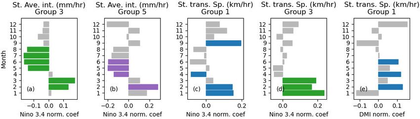
539  Type 2 (T2) storms often move south-eastward and include the fastest and largest storms
540 but with low rainfall intensity. They are frequent during the whole year with a frequency peak in
541 spring
542  Type 3 (T3) storms mostly occur during winter with a frequency peak in June, mostly
543 moving northward over the ocean, and include the very slow storms with the smallest size and
544 low intensity compared to the other types.
545  Type 4 (T4) includes the most extreme storm in terms of rainfall intensity and often
546 appears in large sizes moving eastward with low translation speed. They mostly occur during the
547 summer.
548  Type 5 (T5) storms mostly include very fast storms with small sizes and low rainfall
549 intensities that often occur during the winter, mostly moving northward (over the ocean).
550 To further demonstrate the characteristics of each cluster, a video representing the typical
551 storm for each cluster is provided in the supplemental material (Online Resources 2).
552

553
554
555 Fig. 9 Selected regression coefficients for the relationship between climate mode indices
556 and the object-based storm properties in different months. The detail of selection criteria is
557 explained in the manuscript. The coloured bars show the normalized coefficients that are
558 significantly different from zero. Note that the colours represent the storm groups and are
559 matched with the groups’ colours in figure 8.
560
561 We also investigated whether significant relationships exist between storm properties and
562 climate mode indices. Although no statistically significant relationships were found when
563 investigating all storms, we have found some significant relationships between climate indices
564 and storm properties in each cluster (identified in the previous section) using a multiple
565 regression model described in section 4.3. Based on this approach, 75 regression models have
566 been produced (3 indices × 5 storm properties × 5 clusters). In order to identify robust
567 associations, we have identified instances when at least five coefficients in a row have the same
568 sign (positive or negative), and among them at least three are significantly different from zero.
569 Since these climate indices often have impacts on weather for a period from 3-9 months, this
570 restriction helps us to better exclude those short periods in which precipitation has a statistically
571 acceptable link with climate indices but probably not in reality. Thus, from all of the results, only

 23

572 five regressions passed this criterion and are shown in figure 9. The results show that during El-
573 Niño events in cold seasons, T3 and T5 storms have negative correlation with ENSO in cold
574 season with lower rainfall intensity in El Niño and higher rainfall intensity in La-Niña (fig 9a,
575 9b). ENSO also has an impact on T1 and T3 storms' translation speed during the warm season
576 with a positive correlation (faster in El Niño and slower in La-Niña; fig 9c, 9d). Finally, IOD has
577 also shown to have a positive correlation with T1 storms’ translation speed from mid-summer to
578 early winter (Feb, Apr and Jun; fig 9e). Note that in figure 9, all the coefficients have been
579 normalized to derive the partial correlation between every index and storm property as below:
580
 × ( ℎ ℎ)
581 = (12)
 ( ℎ ℎ)
582
583 Where σ is the standard deviation in this equation, “index coefficient” refers to any
584 calculated coefficient from equation 11 and “index normalized coefficient” is the partial
585 correlation between every index and storm property.

586 5. Discussion
587
588 The results presented in Section 4.1 are broadly consistent with previous studies, but with
589 some notable exceptions. For example, during summer, storms are mostly larger, move faster
590 and are accompanied by higher rainfall intensities compared to the storms in winter (fig 2). This
591 is in agreement with the previous studies over Australia reporting that severe thunderstorms are
592 most prevalent in the warm season (Niall and Walsh 2005; Schuster et al. 2005; Davis and Walsh
593 2008; Warren et al. 2020). The extreme summer and spring storms in terms of rainfall intensity
594 are more intense when they are raining over land between 10:00 to 20:00 (AEST; peaking in the
595 afternoon) compared to when they are raining over the ocean, consistent with the diurnal cycle of
596 surface temperature and the maximum availability of heating over land. The diurnal peak of
597 severe thunderstorm over land during the warm season was also reported by Griffiths et al.
598 (1993) in studying the severe thunderstorms in New South Wales, Australia and Schuster et al
599 (2005) in studying the hail climatology of the Greater Sydney, Australia both using reported
600 data.
601 Although previous studies reported that thunderstorms are more prevalent during the
602 warm seasons, we have found that there are more storms during autumn and winter than spring
603 and summer. A reason behind this contradiction is that most previous studies employed ground
604 observations that provide information for storms only over land (Niall and Walsh 2005; Schuster
605 et al. 2005; Davis and Walsh 2008), and, based on our findings, autumn and winter storms
606 mostly initiate from the ocean and tend to move northward, causing more precipitation over the
607 ocean than land. Thus, the previous studies have not captured the storms over the ocean in these
608 seasons. In addition, most of the previous studies were focused on the severe thunderstorms or
609 storms with deep convective clouds and high storm tops that are often accompanied by

 24

610 electrification, which are less frequent during the cold seasons. Using lightning records, Dowdy
611 and Kuleshov (2014) also showed that a maximum in lightning activity during the cooler months
612 occurs over the ocean to the east of Australia, which is consistent with our results. However, they
613 reported a higher frequency of thunderstorms during the warm season. Since storms in cold
614 season are small-scale with low rainfall intensity, probably many of them are not accompanied
615 by lightning to be captured by the sensors. Therefore, a large number of storms over the ocean
616 during this season are probably missed in the mentioned study.
617 We have calculated the average wind direction during the rainy days (based on radar
618 data) at 700 hPa and 850 hPa in ERA5 Reanalysis data (see fig S6 and S7; Online Resource 1) to
619 examine whether the storm directions are (on average) following the wind directions in different
620 seasons. The results show that typical storm direction in summer and spring seems to be in
621 agreement with climatological wind fields at 700 hPa in ERA5. This agreement seems to be even
622 better when compared with 850 hPa wind fields since the north westerly storm directions (fig 2e,
623 2l) during these seasons are better matched with the wind directions at this pressure level.
624 However, in autumn and winter, it doesn’t seem to agree well, especially over the ocean. Storms
625 in these seasons mostly move northward over the ocean (fig 2e, 2l). However, the average wind
626 directions in these seasons are south-westerly. A reason might be the climatological conditions during
627 the cold season are not supportive of isolated offshore showers/storms which are more frequent in these
628 seasons. However, further investigations are required by conducting a detailed comparison of wind
629 and storm directions.
630 In all seasons, land and ocean-originating storms tend to peak early in their lifetimes (fig
631 6) consistent with the findings of Ayat et. al. (2021b) and Prein et. al. (2017) over the United
632 States. Additionally, we have found that this peak is more prominent during the summer for
633 severe storms raining over land. Storm characteristics also change during the transition of storms
634 between land and ocean like the decrease in max intensity for summertime land-originating
635 storms when moving over the ocean and wintertime ocean-originating storms when moving over
636 land. These variations are probably related to a change in boundary layer instability in this
637 process, and shows the immediate effect of change in air mass characteristics (land/ocean) on the
638 storms. These characteristics can include surface temperature and humidity, sea/land breezes and
639 topographical interactions, the effects of elevated mixed layers advected over the coast, low-level
640 wind shear and convergence.
641 Using clustering analysis, we have found that there are five storm types with similar
642 object-based properties over this region and described in detail in section 5.3. Among these
643 clusters, three storm types might be accompanied by natural disasters, due to their special
644 characteristics. The first storm type (T1) mostly includes the slowest storms that have high
645 rainfall intensities with small areas and mostly move towards the north-northwest with a peak
646 frequency in autumn. These storms can create flash floods if they hit the land like the high
647 impact event that occurred on 30 May 2011 with a dominant contribution of this type of storm
648 and led to flash flooding in some of Sydney's eastern suburbs (e.g., Zetland, Alexandria and
649 Kingsford). T2 storms mostly move towards the southeast and include the largest and fastest
650 storms but with very low rainfall intensity occurring in every season with a peak frequency at the

 25

651 end of spring. This type of storm can be accompanied by severe winds. For instance, they
652 contributed to the storm that occurred on 8 January 2003, and brought a severe wind gust with a
653 maximum of 109 km/h. Finally, T4 storms mostly occur in summer and include the extreme
654 high-intensity storms that have very large sizes with slow translation speed. These characteristics
655 of the storms in this group can create devastating flash and riverine floods in this region (fig 8).
656 Their dominant contribution in the East Coast Low event on 1 and 2 February 2005 caused flash
657 flooding in Sydney with reports of 6 cm size hail.
658 Our results in investigating the relationships between climate mode indices and storm
659 properties are consistent with the previous studies over the eastern and southeastern parts of
660 Australia. Those studies have reported a reduction in rainfall intensity during El-Niño events in
661 the cold season (Chung and Power 2017; Risbey et al. 2009a,b; Murphy and Timbal 2008;
662 Nicholls et al. 1996; McBride and Nicholls 1983; Allan et al. 1996; Schepen et al. 2012; Min et
663 al. 2013; King et al. 2014; Ashcroft et al. 2019). While no relationship was found for all storms,
664 we have found that the rainfall intensity in T3 and T5 storm types (that are more frequent in
665 winter) decreases during these events (fig 9a, b).
666 We have found that there are relationships between some object-based storm properties
667 over the study area that have also been reported in previous studies over other regions. For
668 example, we find that storm objects with large volume and size tend to be more linear and are
669 accompanied by higher rainfall intensities (fig 7); this is consistent with the findings of Ayat et.
670 al. (2021b) in comparing a merged ground radar product and a merged satellite precipitation
671 product over the United States, and Prein et al. (2017) in simulating North American mesoscale
672 convective systems with a convection‑permitting climate model. Large-scale heavy storms over
673 the study area mostly fall in T2 and T4 storm categories, and typical T2 and T4 storms showed
674 that they are mostly frontal systems that elongated/oriented parallel to the front borders.
675 In summary, the results are showing that the storm intensity variations are consistent with
676 diurnal/seasonal cycles and are related to climate mode oscillations. However, other
677 characteristics of the storms like storm size and translation speed do not seem to always follow
678 the same relationship. This suggests that further investigations are required to find a more
679 definitive answer to the effect of atmospheric parameters variations (e.g. temperature, humidity,
680 etc.) on storm properties other than intensity.

681 6. Conclusion
682 In this study, we establish an object-based storm climatology using an S-band weather
683 radar located near Wollongong, NSW (34.26° S, 150.87° E, 471 m altitude) with more than 20
684 years of records (1996-2018). The study area is the radar coverage region (including land and
685 ocean), within 150 km of the radar. Here, we employed the Method of Object-based Diagnostic
686 Evaluation (MODE) Time Domain (MTD) to detect and track the storms. Using this object-
687 based approach helps us to better understand the climatology of storm properties (other than
688 rainfall intensity and frequency) that haven’t been explored in the previous studies over the study
689 area.

 26