Dymola Dymola Release Notes - Dynamic Modeling Laboratory - Claytex
←
→
Page content transcription
If your browser does not render page correctly, please read the page content below
Dymola
Dynamic Modeling Laboratory

 Dymola Release Notes

          Dymola 2019
The information in this document is subject to change without notice.

Document version: 1

© Copyright 1992-2018 by Dassault Systèmes AB. All rights reserved.
Dymola® is a registered trademark of Dassault Systèmes AB.
Modelica® is a registered trademark of the Modelica Association.

Other product or brand names are trademarks or registered trademarks of their respective holders.

Dassault Systèmes AB
Ideon Gateway
Scheelevägen 27 – Floor 9
SE-223 63 Lund
Sweden

Support:         http://www.3ds.com/support
URL:             http://www.Dymola.com
Phone:           +46 46 270 67 00
Contents

1      Important notes on Dymola .................................................................................................... 5
2      About this booklet ................................................................................................................... 5
3      Dymola 2019 ............................................................................................................................. 6
    3.1 Introduction ...................................................................................................................................................... 6
       3.1.1   Additions and improvements in Dymola ................................................................................................ 6
       3.1.2   New and updated libraries ...................................................................................................................... 7
    3.2 Developing a model ......................................................................................................................................... 8
       3.2.1   Support for Modelica 2 in Dymola discontinued .................................................................................... 8
       3.2.2   Capturing the parameter values and other modifiers of a component..................................................... 8
       3.2.3   Filtering of inherited components in diagram....................................................................................... 13
       3.2.4   Improved plotting in the matrix editor .................................................................................................. 15
       3.2.5   Presenting display units in the diagram layer ....................................................................................... 17
       3.2.6   Improved presentation of display units ................................................................................................. 19
       3.2.7   Customizing the File > Libraries menu ................................................................................................ 22
       3.2.8   Adding variables to bus declarations when connecting expandable connectors ................................... 24
       3.2.9   Minor improvements ............................................................................................................................ 26
    3.3 Simulating a model ........................................................................................................................................ 33
       3.3.1   DAE Mode............................................................................................................................................ 33
       3.3.2   Improvements in Variable Browser ...................................................................................................... 34
       3.3.3   Plot window .......................................................................................................................................... 38
       3.3.4   Scripting ............................................................................................................................................... 40
       3.3.5   New features for debugging initialization failures ................................................................................ 40
       3.3.6   Improved nonlinear solver diagnostics ................................................................................................. 44
       3.3.7   Improved initial guesses for nonlinear equations in the model during simulation ............................... 47
       3.3.8   Minor improvements ............................................................................................................................ 48
    3.4 Installation ...................................................................................................................................................... 54
       3.4.1   Dymola as a 32-bit application discontinued ........................................................................................ 54
       3.4.2   Scientific Data Format (SDF) packages for Python and Matlab available on GitHub ......................... 55
       3.4.3   Installation on Windows ....................................................................................................................... 55
    3.5 Other Simulation Environments ..................................................................................................................... 57
       3.5.1   Dymola – Matlab interface ................................................................................................................... 57
       3.5.2   Real-time simulation............................................................................................................................. 57
       3.5.3   FMI Support in Dymola ....................................................................................................................... 58
       3.5.4   Source Code Generation ....................................................................................................................... 66

                                                                                                                                                                           3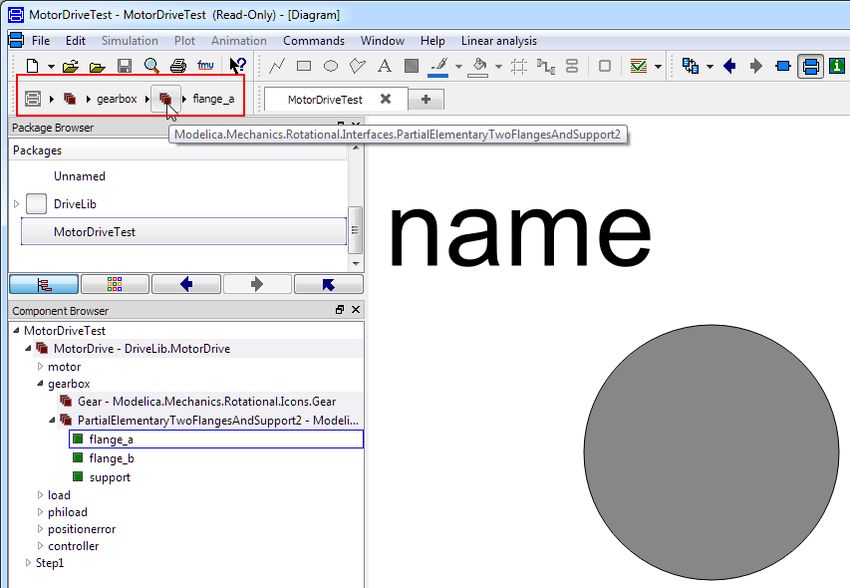
3.6 Modelica Standard Library and Modelica Language Specification ............................................................... 67
    3.7 New libraries .................................................................................................................................................. 67
       3.7.1    ClaRa DCS Library .............................................................................................................................. 67
       3.7.2    Electric Power Systems Library ........................................................................................................... 68
       3.7.3    Pneumatic Systems Library .................................................................................................................. 68
    3.8 Updated libraries ............................................................................................................................................ 70
       3.8.1    Battery Library ..................................................................................................................................... 70
       3.8.2    ClaRa Grid Library ............................................................................................................................... 71
       3.8.3    ClaRa Plus Library ............................................................................................................................... 71
       3.8.4    Cooling Library .................................................................................................................................... 72
       3.8.5    Dymola Commands Library ................................................................................................................. 72
       3.8.6    Electrified Powertrains Library ............................................................................................................ 72
       3.8.7    Fluid Dynamics Library........................................................................................................................ 73
       3.8.8    Fluid Power Library.............................................................................................................................. 73
       3.8.9    FTire Interface Library ......................................................................................................................... 73
       3.8.10   Human Comfort Library ....................................................................................................................... 73
       3.8.11   HVAC (Heating, Ventilation, and Air Conditioning) Library .............................................................. 73
       3.8.12   Hydrogen Library ................................................................................................................................. 73
       3.8.13   Optimization Library ............................................................................................................................ 74
       3.8.14   Testing Library ..................................................................................................................................... 74
       3.8.15   Thermal Systems Library ..................................................................................................................... 75
       3.8.16   VeSyMA (Vehicle Systems Modeling and Analysis) Library.............................................................. 75
       3.8.17   VeSyMA – Engines Library ................................................................................................................. 78
       3.8.18   VeSyMA – Powertrain Library ............................................................................................................ 81
       3.8.19   VeSyMA – Suspensions Library .......................................................................................................... 83
    3.9 Documentation ............................................................................................................................................... 88
    3.10      Appendix – Installation: Hardware and Software Requirements .............................................................. 89
       3.10.1   Hardware requirements/recommendations ........................................................................................... 89
       3.10.2   Software requirements .......................................................................................................................... 89

4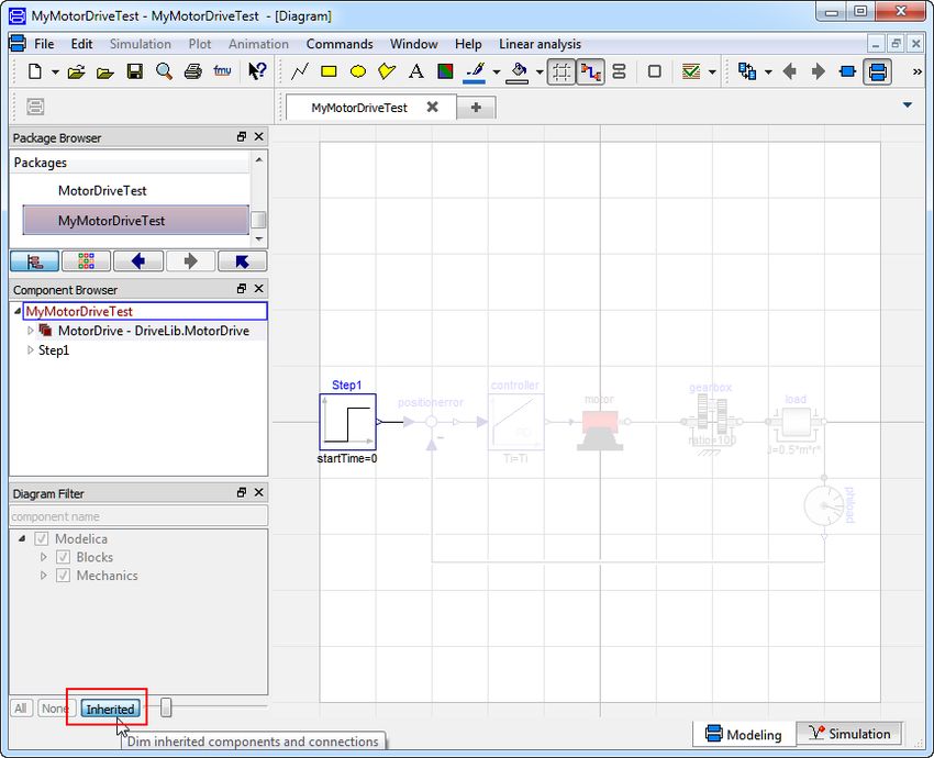
1   Important notes on Dymola
       Installation on Windows
       To translate models on Windows, you must also install a supported compiler. The compiler
       is not distributed with Dymola. Note that administrator privileges are required for
       installation. Three types of compilers are supported on Windows in Dymola 2019:

       Microsoft Visual Studio C++
       This is the recommended compiler for professional users. Note that free Microsoft compiler
       versions earlier than Microsoft Visual Studio Express 2008 are not supported (concerning
       full versions, some earlier versions are supported). Refer to section “Compilers” on page 89
       for more information.

       Intel
       Dymola 2019 has limited support for the Intel Parallel Studio XE compiler. For more
       information about this compiler, see section “Compilers” on page 89; the section about Intel
       compilers.

       GCC
       Dymola 2019 has limited support for the MinGW GCC compiler, 32-bit and 64-bit. For
       more information about GCC, see section “Compilers” on page 89; the section about GCC
       compilers.

       Installation on Linux
       To translate models, Linux relies on a GCC compiler, which is usually part of the Linux
       distribution. Refer to section “Supported Linux versions and compilers” on page 91 for
       more information.

2   About this booklet
       This booklet covers Dymola 2019. The disposition is similar to the one in Dymola User
       Manual Volume 1 and 2; the same main headings are being used (except for, e.g., Libraries
       and Documentation).

                                   Dymola 2019 Release Notes                                    5
3 Dymola 2019
3.1 Introduction
3.1.1 Additions and improvements in Dymola
A number of improvements and additions have been implemented in Dymola 2019. In
particular, Dymola 2019 provides:
• DAE mode for more efficient simulation of large models (page 33)
• Improved initial guesses for equations in the model during simulation (page 47)
• New features for debugging initialization failures (page 40)
• Improved nonlinear solver diagnostics (page 44)
• Capturing parameter values and other modifiers by extending a component to a new
model, or by creating a favorite model from a component (page 8)
• Filtering of inherited components in the diagram layer of editable models (page 13)
• Improved plotting of Boolean and short Integer arrays in the matrix editor (page 15)
• Presentation of display units in the diagram layer (page 17)
• Improved presentation of display units in the parameter dialog (page 19)
• Customization of the File > Libraries menu (page 22)
• Possibility to add variables to bus declarations when connecting expandable
connectors (page 24)
• Variable browser improvements:
o Selecting display units (page 34)
o Improved filtering (page 36)
• Plot improvements (page 38)
o Signal operators for curves plotted against independent variables other
than time
o Improved presentation of display units
• Support for Visual Studio 2017 compiler (page 55)
• Improved FMI support
o General
Reorganization of simulation setup dialog for FMI (page 58)
o FMU Export
Defining user-defined model identifiers for FMUs in GUI
when exporting (page 61)
Sparse Jacobian handling when including source code
supported (page 62)
6
Sparse solver support (page 63)
Export of models in DAE mode (page 63)
More GUI settings available as flags for scripting
o FMU Import
More GUI settings available as flags for scripting
o FMI Kit for Simulink
A new version 2.4.2 with support for Matlab R2017a and
R2017b, and other improvements (page 66)
• Sparse Jacobian handling supported for Source Code Generation (page 66)
• New document: Dymola Referential (page 88)
3.1.2 New and updated libraries
New libraries
The following libraries are new in this Dymola version:
Commercial libraries
• ClaRa DCS Library, version 1.1.0
• Electric Power Systems Library, version 1.0
• Pneumatic Systems Library, version 1.0
For more information about the new libraries, please see the section “New libraries” starting
on page 67.
Updated libraries
The following libraries have been updated:
• Battery Library, version 2.1
• ClaRa Grid Library, version 1.1.0
• ClaRa Plus Library, version 1.1.0
• Cooling Library, version 1.2.1
• Dymola Commands Library, version 1.5
• Electrified Powertrains Library, version 1.2.1
• Fluid Dynamics Library, version 2.5.0
• Fluid Power Library, version 2018.1
• FTire Interface Library, version 1.0.1
• Human Comfort Library, version 2.5.0
• HVAC (Heating, Ventilation, and Air Conditioning) Library, version 2.5.0
• Hydrogen Library, version 1.1
• Optimization Library, version 2.2.3
• Testing Library, version 1.1
Dymola 2019 Release Notes 7
•   Thermal Systems Library, version 1.2.0
           •   VeSyMA (Vehicle Systems Modeling and Analysis) Library, version 2018.1
           •   VeSyMA - Engines Library, version 2018.1
           •   VeSyMA - Powertrain Library, version 2018.1
           •   VeSyMA - Suspensions Library, version 2018.1
         For more information about the updated libraries, please see the section “Updated libraries”
         starting on page 70.

3.2   Developing a model
         3.2.1 Support for Modelica 2 in Dymola discontinued
         Modelica 3.0 was standardized in September 2007 and Modelica Standard Library 3.0 was
         introduced in March 1, 2008. Modelica 2 traces its origins back to 2004.
         The support for Modelica 2 in Dymola is discontinued from Dymola 2018 FD01. Neither
         simulation nor editing of Modelica 2 models is supported. Modelica Standard Library
         (MSL) 2.x is not available.
         Conversion from Modelica 2 to Modelica 3 is still possible in this version, but it is easier to
         verify the conversion in a previous version of Dymola, e.g. Dymola 2018, where Modelica 2
         is still supported. For more information and tips about conversion, see
         MigrationModelica2.pdf.

         3.2.2 Capturing the parameter values and other
               modifiers of a component
         In Dymola 2019 two new commands for capturing parameter values and other modifiers of
         a component are available, Capture Parameters > As Model and Capture Parameters >
         As Favorite. The commands are available as context commands for components in the
         diagram layer and component browser. The context menu in the diagram layer:

8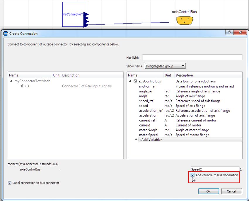
The context menu in the component browser:

                           Dymola 2019 Release Notes   9
Capturing the parameter values of a component by extending to a new
     model
     If you select a component in the diagram layer or component browser, right-click and select
     Capture Parameters > As Model, the component´s model will be extended to create a new
     model. Parameter values and other modifiers are included in the extension.
     As a minor example, consider the following model MyModel with just one parameter
     MyParameter with no default value, however given the value 33 by using the parameter
     dialog:

10
Right-clicking it in the diagram or component browser and selecting Capture Parameters >
As Model, gives the dialog for extending the component´s model. Giving the new model the
name MyModelCapturedParameters in the dialog:
The code of the new model will be:
Instantiating the new model in the diagram and looking at the parameter dialog gives:
Dymola 2019 Release Notes 11Capturing the parameter values of a component by adding a new model to
favorites
If you select a component in the diagram layer or component browser, right-click and select
Capture Parameters > As Favorite, the component will added as a new model to favorites.
Parameter values and other modifiers are included in the new favorite model.
As a minor example, consider the starting point from the example above, the model
MyModel. Now let’s make this model a favorite instead by right-clicking it in the diagram
or in the component browser and select Capture Parameters > As Favorite. The dialog that
appears (if the package to add the favorite model to is selected to be Favorites):
The code for this favorite model will be:
Instantiating this favorite model in the diagram and looking at the parameter dialog gives:
123.2.3 Filtering of inherited components in diagram
The Diagram Filter command has been extended to also include filtering of inherited
components and connections for editable models.
As an example, using the command File > Demos > Motor Drive to open the motor drive
demo, and then using the command New > Duplicate Class… to create an editable model,
you can use the command Edit > Diagram Filter to activate the diagram filter. Now, you
can, in the diagram filter, click Inherited to filter the inherited components of the model:
Dymola 2019 Release Notes 13Notes:
• The model must be editable to be able to do this filtering.
• The Inherited button works in toggle mode.
• If other filtering has been implied in the diagram filter, that filtering is deactivated
(and grayed) while the filtering of inherited components is active. Once the filtering of
inherited components has been deactivated, the previous filtering is active again.
• The opacity level can be changed also for the filtering of inherited components.
• The previous setting Highlight inherited components in the Edit > Options… dialog
has been removed.
143.2.4 Improved plotting in the matrix editor
Support for Boolean and short integer arrays
Boolean and short integer arrays are now plotted as expected; before they were also plotted,
but displayed as real values.
A short integer array is by default defined as an array containing integers where the span
between the minimum value and the maximum value is less than 10. This span can be
changed by changing the value of the flag Advanced.ShortIntegerSpan. (The flag is by
default 10.)
An example of plotting the following short integer array in the matrix editor:
Integer i[:]={1, 2, 0, 4, 8, 8, 7, 4, 3, 3, 6}
The curve is by default displayed using markers, marker style Filled Circle, and only the
original points are marked, not the ones inserted to create the steps.
An example of plotting the following Boolean array in the matrix editor:
Boolean b[:]={true, false, true, true, false}
Dymola 2019 Release Notes 15Support for Line Style and Marker Style for one curve
Plotting in the matrix editor now has support for line style and marker style for the curve in
a plot containing only one curve. You can select using the context menu of the plot:
16Note that for Boolean and short integer arrays that marker (Filled Circle) is the default.
Support for toggling the grid
The grid in a matrix editor plot can be hidden or displayed the same way as in the common
plot window by using the context command Toggle Grid.
3.2.5 Presenting display units in the diagram layer
In Dymola 2019 display units are by default presented in the diagram layer. For example,
the diagram layer of the demo Coupled Clutches now by default looks the following:
Note: The improved presentation of display units described in next section is valid also for
the display units presented in the diagram.
The previous behavior of not presenting the display units in the diagram can be restored by
unticking the setting Use display unit for presenting parameter values, reached by the
command Edit > Options…, the Graphical Editor tab:
Dymola 2019 Release Notes 17This setting is by default ticked. The setting corresponds to the flag
Advanced.UseDisplayUnitInDiagram=true
If unticking the setting, the diagram layer of the demo Couple Clutches will look like in
previous Dymola versions:
183.2.6 Improved presentation of display units
Parameter dialog improvements
Using µ, Ω, and ˚C instead of u, Ohm, and degC
The characters µ, Ω, and˚C are now presented instead of u, Ohm, and degC in the display
unit column. An example of using Ω and ˚C is the pa rameter dialog of an ordinary resistor:
Improved display of e.g. m2 and m3
Power 2 and 3 of units, for example m2 and m3 are now presented in this way, using
Superscript, instead of the previous way presenting m2 and m3.
Dymola 2019 Release Notes 19Entering values with prefixed units
It is possible to enter values with prefixed units, also if that prefix is currently not selectable
from the display unit after the value in the dialog. As an example, consider the parameter
dialog of an ordinary constant current component
(Modelica.Electrical.Analog.Sources.ConstantCurrent):
Default parameter dialog:
Default display unit selection:
20Entering 2 uA (note that you must enter the blank between the value and the unit):
Clicking OK and displaying the parameter dialog again now gives:
The display unit selection has also been updated:
The display unit selection for Ampere will be updated for all display unit selections of
Ampere.
Notes:
• It is possible to enter values with prefixed units also for parameters that have no
alternative display unit (gray background in display unit column).
• The prefixed display unit update is not saved between sessions (the display unit will
still be µA but this selection will not be displayed in the menu for selecting display
unit, that is, that one will be reverted to the default one, until a change is being made
of a µA value).
Dymola 2019 Release Notes 213.2.7 Customizing the File > Libraries menu
In Dymola 2019 you can customize the File > Libraries menu. The new command File >
Library Management has been introduced:
This command contains two tabs. The Libraries tab lets you decide what libraries should be
present in the File > Libraries menu, and the order of the libraries:
22You can:
• Include or exclude all libraries by using the checkbox in the heading
• Include or exclude any library in the list by the checkbox in front of it
• Move the selected library upwards or downwards using the arrow buttons.
Any action is immediately implemented when clicking OK.
The setup is saved between sessions.
To restore the default library configuration, you can click Reset in the menu above.
The second tab Modelica Path is the previous command File > Modelica Path… that has
been included in the Library Management command.
Note. If you change the Modelica Path, by for example adding a directory, the libraries to
select from in the Libraries tab may change when you click OK in the Modelica Path tab.
Dymola 2019 Release Notes 233.2.8 Adding variables to bus declarations when
connecting expandable connectors
It is now possible to add a new variable to the bus declaration when connecting expandable
connectors. This is done by ticking the check box Add variable to bus declaration when
adding a new variable by clicking in the Create Connection menu. An
example:
The next time this dialog is used, for example when connecting to another instance, the new
variable is presented in the bus:
24Note that the check box for adding a variable to the bus declaration is present also for
variables that are visible under when clicking it; ticking the check box for
such a variable will “push” it above the entry in the pane and add it to the
bus declaration.
By default the variables added to bus declarations this way are stored between sessions, this
is controlled by the selection Added variables in bus declarations that can be reached by
the command Edit > Options…, the Settings tab:
Dymola 2019 Release Notes 25If this setting is unticked, the variables added to bus declarations this way will not be present
in the bus declaration dialogs when Dymola is restarted. (The added variables will still be
present in the bus locally for the components where they have been added.)
3.2.9 Minor improvements
Base classes supported in instance hierarchy
Base classes are now supported in the instance hierarchy. As an example, opening the demo
Motor Drive (by File > Demos > Motor Drive) and then right-clicking the gearbox in the
diagram layer and selecting the command Show Component, followed by right-clicking
flange_a and selecting the command Show Component now gives:
26The base classes are shown with the same icon as in the component browser; the name of a
base class can be shown by the tooltip (as above). Just like normal components, base classes
can be navigated to by clicking them in the instance hierarchy.
(To compare, performing the same commands as above in a previous version of Dymola
results in:
Dymola 2019 Release Notes 27)
Shift+double-click on a component in the diagram layer
Previously only double-click was supported on a component in the diagram layer. The
action performed when double-clicking a component in the diagram layer can be configured
using the Edit > Options… command, the Graphical Editor tab. The default action is to
open the parameter dialog of the component.
Now Shift+double-click is also available for a component in the diagram layer. If double-
clicking results in opening the parameter dialog, Shift+double-click on the component will
perform the Show Component command. If double-clicking is configured to do something
else than opening the parameter dialog, Shift+double-click on the component will open the
parameter dialog.
Smart rename and smart delete available as GUI settings
How to update other classes when renaming or deleting a class or a component was
previously available only as flags. Now they are also available in the GUI using the
command Edit > Options…, the Package Browser tab (note than changing any of these
settings does not require a new translation of the model).
28The alternatives for renaming class and renaming components are the same. As example,
looking at renaming classes:
The alternatives correspond to the alternatives of the flags
Advanced.ActivateSmartRenameClass (for renaming classes), and
Advanced.ActivateSmartRename (for components):
Dymola 2019 Release Notes 29GUI alternative Flag value
No 0
Ask in dialog 1
Yes [default] 2 [default]
Yes, also conversion scripts 3
Notes:
• In the dialog you get when having selected Ask in dialog, you can change the setting
to Yes for future renaming by ticking Always update without confirmation and then
clicking Update.
• In the last alternative, “also conversion scripts” means that the renaming operations
are accumulated in a conversion-script, to enable conversion of libraries using the
library that were not loaded during the conversion.
The alternatives for deleting classes or component correspond to the alternatives of the flag
Advanced.ActivateSmartDelete:
GUI alternative Flag value
No 0
Ask in dialog [default] 1 [default]
Yes, if possible 2
Note that in the dialog you get when having selected Ask in dialog, you can change the
setting to Yes for future renaming by ticking Always update without confirmation and
then clicking Update
The Edit > Options… dialog contains a new tab
The dialog from the command Edit > Options… now contains a new tab Package Browser.
The tab contains settings related to the package browser previously located in the General
tab, as well as new settings related to updates of classes when, for example, renaming a
class. See previous section for details about these new settings.
The General tab and the Package Browser tab now looks the following:
30Shortcuts for navigating model tabs
Having a number of model tabs, Ctrl+Tab activates the tab to the right of the currently
active tab in the model tabs toolbar; corresponding to moving down in the list of tabs
(available to the right in the model tabs toolbar). Ctrl+Shift+Tab activates the tab to the left
of the currently active one, corresponding to moving up in the list of tabs.
Simplified insertion and editing of links in the documentation layer
The insertion and editing of links in documentation has been simplified:
• When creating a link using the toolbar button Link , from a text that is a web
address, the dialog for creation is prepopulated:
Dymola 2019 Release Notes 31• If you have entered something that can be identified as a link in the text in the
documentation layer and if you continue with pressing press Space, Enter or Tab, a
link is automatically created. This feature can be disabled by setting the flag
Advanced.AutoLinksDoc = false.
• To edit an existing link, you can place the cursor anywhere on the link, click the Link
button in the toolbar, and edit the link or remove it by ticking Remove link.
MathML supported for inserting and editing equations and expressions in
the documentation layer
You can now also use MathML format when inserting and editing equations and
expressions in the documentation layer using the toolbar button Equation .
The MathML expression needs to be surrounded with … or
…. An example:
Opacity in diagram filter saved between sessions
The diagram filter, activated by, for example, Edit > Diagram Filter, includes a slider to set
the opacity of the components being filtered out. This setting can now also be controlled by
the flag Advanced.DiagramFilterOpacity. The default value is 0.15. The value of the
flag is saved between sessions.
32File > Modelica Path… integrated in File > Library Management
The previous command File > Modelica Path… is now integrated in the new command File
> Library Management, as the second tab Modelica Path. No other changes have been
made for this command.
3.3 Simulating a model
3.3.1 DAE Mode
Dymola 2019 supports DAE (Differential-Algebraic Equations) mode. DAE mode is
activated by setting the flag
Advanced.Define.DAEsolver = true
DAE mode is supported by the integrators Dassl, Radau IIa, Esdirk23a, Esdirk34a,
Esdirk45a, and Sdirk34hw. (The flag is by default false.)
A translated model may contain several nonlinear equation systems. (These are listed in the
translation log under Statistics.) When DAE solver is not enabled these equations are solved
numerically whenever the integrator calls the model. When DAE solver is enabled the
equations in the output and dynamics section of the model are not solved during calls to the
model. They are instead handled by the integrator as part of the nonlinear system of
equations that the integrator solves each step. If the translated model contains several or
large nonlinear equation systems, then DAE solvers may be more efficient since fewer
nonlinear systems are solved.
When a simulation is run with the DAE flag enabled and one of the above solvers are used a
message is printed in the simulation log. The message
The translated model is a DAE. Integrating using DAE solver.
means that there are nonlinear equations in the output and/or dynamics section of the
translated model and that these are handled by the integrator as described above. The
message
The translated model is an ODE. Integrating using DAE solver.
means that there are no nonlinear equations in the output and dynamics section of the
translated model. However, the DAE solver formulation is still used. In this case, no
performance differences should be expected compared to simulation without the flag
enabled.
When trying to run a simulation in DAE mode with a solver that is not supporting DAE
mode, the simulation is terminated and an error message is printed.
It is allowed to export a model where the DAE flag is set but the selected solver does not
support DAE mode using Binary Model Export or Source Code Generation, but the model
will generate error messages when trying to simulate it.
Dymola 2019 Release Notes 33However, it is not allowed to export such a model as an FMU, neither as an FMU using
model exchange or as an FMU using co-simulation. Trying to perform such an export, an
error message is given.
3.3.2 Improvements in Variable Browser
Selection of display units
In Dymola 2019, you can select display units for signals in the variable browser, if display
units are defined for the signals, and if the signals are editable. Click on the unit to get a
selection like in the parameter dialog:
When you have selected the new display unit the value is converted.
When you plot the signal, the selected display unit is used in the plot.
Context command to close all results in the variable browser
For the top-level nodes in the variable browser, a new context command Close All Results
can be given.
34The command closes all results; however the initial values of the current model are still
present. This facilitates giving new initial values to be able to make a re-simulation with
better parameter settings.
Dymola 2019 Release Notes 35If a new model is opened now, also the initial values will be closed, since they do not apply
to the new model.
The behavior is the same as for the built-in function removeResults(). This function is
available also in previous versions.
Option to decide if filtering should be case sensitive or not, and changed
default value
In Dymola 2019 it is possible to decide if the filtering using the line at the bottom of the
variable browser should be case sensitive of not. This can be changed by the command
Case Sensitive in the context menu of the filter line:
36By default the filtering is not case sensitive – this is changed from previous versions of
Dymola where the filtering was case sensitive. Clicking the command gives (the command
works in toggle mode):
Dymola 2019 Release Notes 37When starting a new session, the filtering is always not case sensitive.
The results of a failed initialization can be made available in the variable
browser
The results of a failed initialization can be made available in the variable browser. See “The
results of the failed initialization can be plotted using the Variable Browser” on page 42.
3.3.3 Plot window
Signal operators for curves plotted against independent variables other
than time
You can now apply signal operators on curves plotted against independent variables other
than time. All signal operators are supported, except First Harmonic, Total Harmonic
Distortion (THD), and FFT (Fast Fourier Transform).
An example:
Only independent variables with values rising over time are supported. Trying to apply a
signal operator on an independent variable not fulfilling this will produce an error message.
Creating the supported signal operators by scripting, using plotSignalOperator or
plotSignalDifference also works.
38Command to close all plot windows
The new command Plot > Close All Plot Windows closes all plot windows in the current
Dymola window.
Note that if you have opened a second Dymola window from the current one (by the
command Window > New Dymola Window) only the plots in the window where the new
window command was issued will be closed.
Display unit presentation in plots improved
The improved display unit presentation in the parameter dialog is also implemented in the
plot. The improvements consist of:
• Displaying µ, Ω, and ˚C instead of u, Ohm, and degC
• Displaying power 2 and 3 using Superscript e.g. presenting m and m instead of m2
2 3
and m3
• Displaying units with new prefix that have been used to enter the values, for example,
having entered 10 kOhm instead of 10000 for a variable with unit Ohm, this value will
be displayed as 10 kΩ or 10 kOhm.
These improvements are implemented for the curve and parameter tooltips, the legend, axis
headings, and the curve context command Display Unit. For details on the improvements,
see relevant parts of “Parameter dialog improvements” on page 19.
Note! Presently the variable browser is still unchanged, entering and presenting values has
to be done as in previous versions.
Dymola 2019 Release Notes 393.3.4 Scripting
New built-in function GetDymolaCompiler (Windows)
A new built-in function GetDymolaCompiler has been added. The function extracts the
compiler settings from the Compiler tab of the simulation setup (except the Customer
options settings) to two output text parameters, compiler that is the compiler type, and
settings[:] that contains the other settings. An example of a call and the output of that
call:
GetDymolaCompiler()
= "vs", {"CCompiler=MSVC", "IntelDir=C:/Program Files
(x86)/IntelSWTools/compilers_and_libraries_2016.1.146",
"IntelVsVersion=", "GCC32Path=C:/MinGW/bin/gcc.exe",
"GCC64Path=C:/MinGW64/mingw64/bin/gcc.exe",
"MSVCDir=C:/Program Files (x86)/Microsoft Visual Studio
14.0/Vc",
"gcc32Disabled=0", "gcc64Disabled=0", "DDE=0", "DLL=0",
"OPC=0"}
(The Customer options settings in the Compiler tab cannot be extracted by this function;
they are handled by the string flags Advanced.LinkerOptions and
Advanced.CompilerOptions, respectively.)
Note that the function extracts all settings except the above, not only the ones used.
The function can be used, for example, to test if an application relying on a specific
compiler setup is supported on a certain machine by defining and populating the variables
compiler and settings by the call (compiler,settings)=GetDymolaCompiler()
and then comparing with demands.
The function is not supported on Linux; in Linux it returns just an empty list.
The function is available in the DymolaCommands library.
Note the related built-in function SetDymolaCompiler that can be used to define the
compiler settings.
Improved built-in functions for signal operators
The built-in functions plotSignalOperator and plotSignalDifference have been
extended to also work creating signal operators for curves plotted against independent
variables other than time; with certain limitations. See “Signal operators for curves plotted
against independent variables other than time” on page 38 for the limitations.
3.3.5 New features for debugging initialization failures
Activating the features
To activate the features below, you must, before the simulation, enable the new setting
Store variables after failed initialization in the simulation setup. You can reach this setting
by the command Simulation > Setup…, the Debug tab:
40The setting is by default not enabled. The setting is saved between sessions; see also “Minor
changes in the Debug tab in simulation setup, and more settings saved between sessions” on
page 53.
Plot Dependencies available also after failed initializations
You can now use the feature of plotting dependencies also after failed initializations, if you
have activated the setting in previous section before simulation. The feature is available in
the same way as usual, note however that the presented dependencies are for the simulation
problem, the dependencies for the initialization problem may differ, cf. dsmodel.mof.
Dymola 2019 Release Notes 41The results of the failed initialization can be plotted using the Variable
Browser
If you have activated the setting in the first subsection above before simulation, after a failed
initialization all variables are now available in the Variable Browser, ready for plotting. The
value of each variable depends on how far the initialization process came before failing. If
the variable was initialized the result of that initialization is presented. If the variable was
not initialized its start value is instead presented. The simulation log contains information on
what made the initialization fail. The execution order can be found in e.g. dsmodel.mof (to
generate this file, activate the setting Generate listing of translated Modelica code in
dsmodel.mof before translation, the setting can be reached by the command Simulation >
Setup…, the Translation tab).
Consider the example model:
To compute the variable der(x) = dx Dymola will, during translation, generate a nonlinear
equation in this variable. When simulating the model Dymola complains that it cannot solve
this nonlinear equation and the initialization fails. Plotting the iteration variable der(x) = dx
gives the last attempted value in the Newton iteration.
42By a closer look at the model one can see that the nonlinear equation depends on the
variables u and x. (This information is also readily available in the translation log if you
enable the setting List non-linear iteration variables before translation, the setting can be
reached by the command Simulation > Setup…, the Translation tab) or in dsmodel.mof
(see above how to generate this file).) Plotting these variables reveals that u = 0 and x = -
0.5.
Dymola 2019 Release Notes 43Thus, the nonlinear equation reduces to exp(dx) = -0.5, which lacks solution. The source of
the initialization problem has been isolated.
Also note that a look into dsmodel.mof reveals that y1 is computed before the attempt to
solve the nonlinear equation. The variable y2 is computed after. This agrees with the values
presented when plotting these variables: y1 = -0.125 and y2 = -1. The former variable has it
computed value x^3, whereas the latter variable has its start value -1.
3.3.6 Improved nonlinear solver diagnostics
The message in the simulation log when there is a failure to solve nonlinear equations has
been improved:
More general information
When there is a failure to solve nonlinear equations, the general message contains:
• More information about common causes for failures
• Extended list of settings that can be used to get more information, for example, the
new settings in section “New features for debugging initialization failures” starting on
page 40.
• A nonlinear solver summary, if the below option is activated.
44Option to print a nonlinear solution summary
A new setting Nonlinear solution summary is available in the simulation setup. This
setting is reached by the command Simulation > Setup…, the Debug tab:
The setting is by default not activated. If activated, a summary of the nonlinear solution is
generated in the simulation log. An example:
Dymola 2019 Release Notes 45If the above setting is active, the nonlinear solution summary is also included in the message
given in the simulation log in the following cases:
• When solving a nonlinear equation fails
• When initialization fails
• When using profiling – note the tip about setting the flag
Advanced.GenerateBlockTimers to activate profiling to log CPU times, see also
“Improved profiling information” on page 51.
More information when using the setting Nonlinear solution in the
simulation setup
If the setting Nonlinear solution in the simulation setup has been activated before
translation, the information has been enhanced with:
• How many times each nonlinear equation is called
• A nonlinear solver summary, displaying accumulated results, if the setting Nonlinear
solution summary has been activated.
(The simulation setup can be reached by the command Simulation > Setup…, the Debug
tab.)
463.3.7 Improved initial guesses for nonlinear equations
in the model during simulation
A translated Modelica model may contain nonlinear equations which are solved several
times during integration. To enable fast and robust solution Dymola integrators provide
initial guesses for these nonlinear equations. The guesses are dynamically updated during
integration to incorporate the most recent values of the iteration variables of the nonlinear
equation system.
In Dymola 2019 these initial guesses have been further improved, in particular for nonlinear
equations in the accepted sections (Accepted Section and Conditionally Accepted
Section) of the model equations.
(To display the output of manipulated equations in readable form to see the different
equations sections, you must generate the output of manipulated equations in Modelica
format and investigate the file dsmodel.mof. For more information about this, and
examples, see Dymola User Manual Volume 1, section 5.5.6 “Output of manipulated
equations in Modelica format”.)
The inter-/extrapolation method to be used to compute initial guesses can be controlled by
using the flag
Advanced.Define.InitialGuessInterpolation
The flag can have any of the following values:
• 0 results in constant inter-/extrapolation in all sections
• 1 (default) meaning linear inter-/extrapolation is being used to define initial guesses in
all sections except accepted sections
• 2 results in linear inter-/extrapolation only in accepted sections
• 3 results in linear inter-/extrapolation being used to define initial guesses in all
sections.
Linear extrapolation typically performs better if the iteration variables vary smoothly as
functions of time, otherwise constant extrapolation may perform better.
Note that only some solvers support linear inter/extrapolation. The solvers supporting it are
• Dassl
• Radau IIa
• Esdirk23a, 34a, and 45a
• Dopri45 and 853
• Sdirk34hw
• Cerk23, 34, and 45
Enabling the flag
Advanced.MoveEquationsToDynamics
moves all nonlinear equations in the accepted sections to the dynamics section. This may be
useful if problems with nonlinear equations in the accepted sections are experienced,
Dymola 2019 Release Notes 47especially if few output points are used. It forces the integrator to solve the nonlinear
equations each integrator step and thereby it also updates the initial guesses more often.
3.3.8 Minor improvements
Alias elimination of parameters
In Dymola 2019 alias elimination of parameters can be obtained, by setting the flag
Advanced.AllowParameterAlias=true
This eliminates parameters equal to other parameters – in the same way as alias elimination
of time-varying variables. This is primarily intended to reduce the size of the generated C-
code, and the only down-side is that such parameters are treated a bit specially when
exporting the model to FMI.
Efficient code generation for large tables
Large tables in Modelica models will by default yield a large amount of extra C code to be
compiled and fills up the variable browser with table data which may be of limited interest.
In Dymola 2019 it is possible to avoid this overhead by setting the annotations
Evaluate=true and HideArray=true on the table, combined with the new (see above
section) global setting Advanced.AllowParameterAlias=true. For example,
Setting to use analytic ODE Jacobians available in GUI
In previous versions, to use analytic ODE Jacobians during simulation and also for
linearization, you could set the flag Advanced.GenerateAnalyticJacobian to true.
Now there is a corresponding setting Generate Analytic Jacobian for the OED problem
available in the GUI, in the simulation setup, the Translation tab:
48(The simulation setup can be reached by the command Simulation > Setup…)
The setting is by default not activated.
The setting is intended to improve the simulation speed, by computing the Jacobians more
efficiently, but it generates a large amount of C code that needs to be compiled. Note that
the speed improvement may not be as large as assumed since that case when the setting is
not activated has also been optimized.
More efficient event handling activated by default
Already in previous Dymola versions a more efficient event handling of “minor” events
could be activated by setting the flag Advanced.EfficientMinorEvents = true. In
Dymola 2019 Release Notes 49Dymola 2019, this is the default value, since generally having this feature activated is a
gain.
Extended information about nonlinear systems of equations in the
translation log
In Dymola 2019, if activating the setting List non-linear iteration variables in the
simulation setup (reached by the command Simulation > Setup…, the Translation tab) the
following information is now also listed in the translation log when translating the model:
• Initial equations (previously only simulation equations were listed)
• Time-varying variables that the equations depend on (previously only the iteration
variables were listed)
• Each system of equations is more precisely tagged
As an example, please compare the last part of the translation log for the model
Modelica.Mechanics.Multibody.Examples.Loops.EngineV6 for Dymola 2019 (to the left)
and Dymola 2018 FD01 (to the right):
Improved logic for concealing parts of model.mof and dsmodel.mof
The logic for concealing parts of model.mof and dsmodel.mof depending on encryption
and the annotation showDiagnostics has been improved.
50Improved profiling information
In the profiling information, given in the simulation log when the flag
Advanced.GenerateBlockTimers is set to true before simulation, the tags for linear
and non-linear equation systems are now used.
Changed usage of compiled functions
In Dymola 2019 expressions using compiled functions are not evaluated unless needed, for
example, if they contain any parameter with the annotation Evaluate=true.
For compatibility reasons, if models have been constructed to rely on all expressions using
compiled functions being evaluated, previous behavior can be preserved by setting the flag
Advanced.RelyOnCompiledFunctions=true
The flag is false by default.
Several result files can be opened by multiselection
The plot and animation commands for opening result files (Plot > Open Result… and
Animation > Open Result…) now supports opening several result files by multiselection
using Shift or Ctrl keys the usual way.
Note that the opened result files will be displayed in alphabetical order in the variable
browser.
Shortcuts for navigating recent windows
Having a number of subwindows in a Dymola window (plot, animation, diagram, visualizer
window), the already previously available command button Recent Windows can display a
list of these by clicking the arrow to the right of the button. Now shortcuts are available for
navigation in that list: Ctrl+Tab activates the subwindow below the currently active one in
the list, while Ctrl+Shift+Tab activates the subwindow above the currently active one in the
list.
Progress bar in the taskbar icon for Dymola (Windows)
When you simulate, you now get a progress bar in the taskbar icon for Dymola. During
initialization, you get a green blob that moves back and forth. During simulation you get a
progress bar based on the current simulation time. In the example below the max time was
set to 2000 s.
Dymola 2019 Release Notes 51Note that this progress bar is currently only available in Windows.
Improved editing in the command window
Option to hide the toolbar of the command window
In Dymola 2019 a new context command Show Toolbar makes it possible to display/hide
the toolbar of the command window to save screen space:
The toolbar is shown by default. The command works in toggle mode. If Show Toolbar is
not activated, the command window looks like:
The setting is saved between sessions.
Command button to enable/disable mathematical notation in the command log
A new command button in the command window toolbar can be used to enable/disable
mathematical notation in the command log. The button works in toggle mode.
52The mathematical notation includes formulas and equations, Greek characters, and index
rendering.
In the example above, the expression with beta has been entered with mathematical notation
disabled, while the expression with gamma has been entered with mathematical notation
enabled. Note that the flag controlling Greek character rendering
(Advanced.RenderGreekLetters) is simply overrun when the mathematical notation is
disabled; the value of the flag does not matter here.
By default the mathematical notation is disabled. This setting corresponds to the flag (which
was available also in previous versions):
Advanced.MathematicalNotation.InCommandLog = false
The setting is saved between sessions.
Simplified insertion and editing of links in the command log
The insertion and editing of links in the command log using the command button Link in
documentation editor has been simplified in the same way as when doing this in the
documentation layer. See section “Simplified insertion and editing of links in the
documentation layer” starting on page 31 for details.
MathML supported for inserting and editing equations and expressions in the
command log
You can now also use MathML format when inserting and editing equations and
expressions in the command log using the command button Equation, in the same way as
doing this in the documentation layer. See section “MathML supported for inserting and
editing equations and expressions in the documentation layer” starting on page 32.
Editing of inserted equations and expressions harmonized with the corresponding
command in the documentation layer
In Dymola 2019, to edit an inserted equation/expression that has been inserted using the
toolbar command button Equation, put the cursor directly in front of, or directly after the
equation/expression and then click the command button Equation; this will bring up the edit
dialog again - this is the same way to do it as in the documentation layer.
Minor changes in the Debug tab in simulation setup, and more settings
saved between sessions
The settings in the Debug tab in the simulation setup (reached by Simulation > Setup…,
the Debug tab) have been slightly rearranged, and all settings in the General group are now
saved between sessions.
Dymola 2019 Release Notes 533.4 Installation
For the current list of hardware and software requirements, please see chapter “Appendix –
Installation: Hardware and Software Requirements” starting on page 89.
3.4.1 Dymola as a 32-bit application discontinued
Dymola 2018 was the last version to support Dymola as a 32 bit application. Dymola 2018
FD01 and later versions are only available as 64-bit applications, on Windows and Linux.
54Note however that only the Dymola 32-bit application is discontinued, the executable
dymosim.exe, for example, is still available as a 32-bit executable.
3.4.2 Scientific Data Format (SDF) packages for Python
and Matlab available on GitHub
The Scientific Data Format (SDF) packages for Python and Matlab have been removed from
the Dymola distribution; they are now instead available on GitHub:
Removed package Now available on
bin\external\Python https://github.com/ScientificDataFormat/SDF-Python
Mfiles\+SDF https://github.com/ScientificDataFormat/SDF-MATLAB
3.4.3 Installation on Windows
For the full list of supported compilers, see “Software requirements” starting on page 89.
Support for Visual Studio 2017 compiler
Dymola 2019 supports the Visual Studio 2017 compiler, the following editions:
• Visual Studio 2017 Desktop Express Note! This compiler only supports compiling to
Windows 32-bit executables.
• Visual Studio Community 2017
• Visual Studio Enterprise 2017
• Visual Studio Professional 2017
The recommended free compiler to use is the Community edition due to the limitation in the
Desktop Express edition.
The compiler is selected in the simulation setup, reached by the command Simulation >
Setup…, the Compiler tab:
Dymola 2019 Release Notes 55You can also read


