Volcanic ash forecast using ensemble-based data assimilation: an ensemble transform Kalman filter coupled with the FALL3D-7.2 model ETKF-FALL3D ...
←
→
Page content transcription
If your browser does not render page correctly, please read the page content below
Geosci. Model Dev., 13, 1–22, 2020
https://doi.org/10.5194/gmd-13-1-2020
© Author(s) 2020. This work is distributed under
the Creative Commons Attribution 4.0 License.

Volcanic ash forecast using ensemble-based data assimilation: an
ensemble transform Kalman filter coupled with the FALL3D-7.2
model (ETKF–FALL3D version 1.0)
Soledad Osores1,2,3 , Juan Ruiz4 , Arnau Folch5 , and Estela Collini6
1 Servicio Meteorológico Nacional (SMN), Buenos Aires, Argentina
2 Consejo  Nacional de Investigaciones Científicas y Técnicas (CONICET), Buenos Aires, Argentina
3 Comisión Nacional de Actividades Espaciales (CONAE), Buenos Aires, Argentina
4 Centro de Investigaciones del Mar y la Atmósfera, Facultad de Ciencias Exactas y Naturales, Universidad de Buenos Aires,

CONICET, UBA, UMI-IFAECI (CNRS-CONICET-UBA), Departamento de Ciencias de la Atmósfera y los Océanos,
Facultad de Ciencias Exactas y Naturales, Universidad de Buenos Aires. Buenos Aires, Argentina, Argentina
5 Barcelona Supercomputing Center (BSC), Barcelona, Spain
6 Servicio de Hidrografía Naval (SHN), Buenos Aires, Argentina

Correspondence: Soledad Osores (msosores@smn.gob.ar)

Received: 9 April 2019 – Discussion started: 3 June 2019
Revised: 29 October 2019 – Accepted: 31 October 2019 – Published: 2 January 2020

Abstract. Quantitative volcanic ash cloud forecasts are prone        1   Introduction
to uncertainties coming from the source term quantification
(e.g., the eruption strength or vertical distribution of the emit-
ted particles), with consequent implications for an opera-           Volcanic ash dispersal forecasts are routinely used to pre-
tional ash impact assessment. We present an ensemble-based           vent aircraft encounters with volcanic ash clouds and to de-
data assimilation and forecast system for volcanic ash disper-       fine flight rerouted trajectories, avoiding potentially contam-
sal and deposition aimed at reducing uncertainties related to        inated airspace areas. In the aftermath of the 2010 Eyjafjalla-
eruption source parameters. The FALL3D atmospheric dis-              jökull volcanic eruption in Iceland, safety-based quantitative
persal model is coupled with the ensemble transform Kalman           criteria for air traffic disruption were introduced, originally
filter (ETKF) data assimilation technique by combining ash           based on ash concentration thresholds and, more recently, on
mass loading observations with ash dispersal simulations in          engine-ingested dosage (Clarkson et al., 2016). These sce-
order to obtain a better joint estimation of the 3-D ash con-        narios involve the implementation of quantitative ash con-
centration and source parameters. The ETKF–FALL3D data               centration forecasts, which require better model input con-
assimilation system is evaluated by performing observing             straints, particularly on ash emission rates and/or on model
system simulation experiments (OSSEs) in which synthetic             initialization. A large amount of scientific research has been
observations of fine ash mass loadings are assimilated. The          conducted in recent years to achieve the following: (i) better
evaluation of the ETKF–FALL3D system, considering refer-             quantify the amount of ash emitted, its vertical distribution
ence states of steady and time-varying eruption source pa-           across the column, and the related uncertainties; (ii) obtain
rameters, shows that the assimilation process gives both bet-        data on the 3-D structure of ash clouds, particularly using
ter estimations of ash concentration and time-dependent op-          ground, aircraft, and space-based instrumentation; (iii) im-
timized values of eruption source parameters. The joint es-          prove model representation of the physical processes occur-
timation of concentrations and source parameters leads to a          ring within ash plumes and clouds; and (iv) transfer scientific
better analysis and forecast of the 3-D ash concentrations.          outcomes into operations. However, despite the substantial
The results show the potential of the methodology to improve         advances in model formulation and initialization, it is esti-
volcanic ash cloud forecasts in operational contexts.                mated that, in operational contexts, forecasted ash concen-

Published by Copernicus Publications on behalf of the European Geosciences Union.
2                                                                                         S. Osores et al.: ETKF–FALL3D v1.0

trations can still have an uncertainty as large as 1 order of       of ash concentrations. Fu et al. (2017b) presented a modified
magnitude (e.g., IVATF, 2011).                                      approach for comparison between models and observations
   Epistemic uncertainties in ash dispersal forecasts may           in the context of the ensemble Kalman filter that tries to deal
have different origins, including the following: (i) uncertain-     with this limitation.
ties in the source term (i.e., eruption column height, mass            Uncertainties in the source parameters can be circum-
eruption rate, particle grain size distribution); (ii) uncertain-   vented in part by using inverse modeling techniques for the
ties in the atmospheric model driving dispersal simulations         optimization of these parameters. Eckhardt et al. (2008) im-
(e.g., wind velocity and direction, small-scale turbulence in-      plemented a source parameter optimization approach based
tensity, atmospheric temperature, and humidity); and (iii) un-      on the definition of a cost function that measures the de-
certainties in model parameterizations of the physical pro-         parture of ash concentrations from observed values and the
cesses occurring both in the eruptive column and during             departure of the estimated parameters from their a priori val-
subsequent passive transport (e.g., ash settling and removal        ues. This allowed for the reconstruction of the full emission
processes, particle aggregation, interaction with meteorolog-       profile using data from different sensors. Stohl et al. (2011),
ical clouds, etc.). In addition to these, aleatoric uncertainties   Kristiansen et al. (2012), Denlinger et al. (2012), Pelley et al.
always exist regarding the future evolution of the eruption         (2015), and Steensen et al. (2017) discussed further develop-
source parameters (ESPs) when an eruption is ongoing at             ments and evaluations of the proposed approach. In particu-
the time of running a forecast. Several studies (e.g., Zehner,      lar, Pelley et al. (2015) describe the operational implementa-
2010; Kristiansen et al., 2012) have concluded that the main        tion of this algorithm at the London Volcanic Ash Advisory
source of epistemic uncertainty in ash dispersal forecasts          Centre (VAAC). In Chai et al. (2017), the optimal parameters
comes from ESPs that very often are not well constrained            are found using a quasi-Newtonian minimization approach of
in real time.                                                       a similar cost function, and Lu et al. (2016) use a similar ap-
   Inverse modeling and, in particular, data assimilation           proach in the context of an Eulerian model. Finally, Zidikheri
methods are techniques that can be used to estimate the state       et al. (2017a, b) presented an optimization algorithm based
of dynamical systems based on partial and noisy observa-            on a systematic search of the optimal parameter values for
tions. In a broad sense, these techniques build on continu-         both qualitative and quantitative ash forecasts and evaluated
ous or quasi-continuous observations to produce model ini-          the performance of the technique for different cases, showing
tial conditions (analyses) that can be used to better predict       a positive impact on forecast quality. Wang et al. (2017) per-
the future state, taking into account uncertainties in observa-     form idealized experiments in which a particle filter and an
tions and model formulation. Data assimilation methods have         expectation maximization algorithm are used for the estima-
been successfully applied to the estimation of the state of the     tion of ash source parameters, obtaining promising results.
ocean or the atmosphere (e.g., Kalnay, 2003; Carrassi et al.,          The goal of this paper is to contribute to the development
2018) as well as for the optimization of uncertain model pa-        of data assimilation methods to improve quantitative ash
rameters (e.g., Ruiz et al., 2013). More recently, applications     dispersion forecasts. To this end, we propose an ensemble-
have been extended to atmospheric constituents (e.g., Boc-          based data assimilation system for volcanic ash combining
quet et al., 2010; Hutchinson et al., 2017), including ash dis-     an ensemble transform Kalman filter (ETKF) (Ott et al.,
persion models with the purpose of estimating the 3-D dis-          2004; Hunt et al., 2007) and the FALL3D ash dispersal
tribution of ash concentrations to be used as initial condi-        model (Costa et al., 2006; Folch et al., 2009), named ETKF–
tions for forecasts. Surprisingly, examples of the application      FALL3D. This system produces a joint estimation of 3-D
of data assimilation techniques to volcanic ash dispersion are      ash concentration and critical ESPs that can improve the
scarce and still mainly limited to a research level. For ex-        performance of classical ash dispersion forecast strategies.
ample, Wilkins et al. (2015) implemented a data insertion           This paper presents a first analysis of the ETKF–FALL3D
methodology to improve the initial conditions of ash concen-        system using different observing system simulation experi-
trations based on satellite estimations of ash mass loadings        ments (OSSEs) in which synthetic observations of ash col-
in a Lagrangian dispersion model. Fu et al. (2015, 2017a)           umn mass loadings are simulated and assimilated. The sys-
applied an ensemble Kalman filter technique to the estima-          tem is evaluated under constant and time-dependent ESPs,
tion of ash concentrations in an Eulerian dispersion model          and the sensitivity of the system performance to parame-
based on flight concentration measurements and satellite es-        ter uncertainty, ensemble size, and observation uncertainty
timations using idealized experiments and real observations.        is explored and discussed. Additionally, some impacts of the
Their results showed that both observational sets (flight mea-      Gaussian assumptions underlying the ensemble Kalman fil-
surements and satellite mass loads) reduced forecast errors,        ter in the present case are discussed. A description of the
which in their particular case were attributed to a wrong           methodology is presented in Sect. 2, the experimental setup
model representation of ash sedimentation processes. One            of the sensitivity experiments is described in Sect. 3, the re-
important issue when using satellite estimates of ash mass          sults are discussed in Sect. 4, and the final conclusions are
loadings is that observations only provide a 2-D distribution       outlined in Sect. 5.
of ash mass, while models usually require the vertical profile

Geosci. Model Dev., 13, 1–22, 2020                                                        www.geosci-model-dev.net/13/1/2020/
S. Osores et al.: ETKF–FALL3D v1.0                                                                                                 3

2     Methodology                                                    parameters in terms of the deposit has been documented by,
                                                                     e.g., Scollo et al. (2008).
2.1    The FALL3D model
                                                                     2.2   The ETKF–FALL3D system
FALL3D is an Eulerian atmospheric dispersal model that
solves the advection–diffusion–sedimentation equation for a          In operational applications, data assimilation is implemented
set of particle classes (bins), each characterized by a parti-       sequentially to provide an estimation of the state of the sys-
cle size, density, and shape factor. Given an eruption source        tem at a series of times in the so-called “data assimilation
term and meteorological variables, FALL3D solves the 4-D             cycle”. Each data assimilation cycle consists of two steps: a
ash concentration for each particle class, from which the to-        first step in which the numerical model is used to provide
tal and the fine ash column mass loadings are diagnosed by           an a priori estimation or forecast of the state of the system
performing a vertical integration. The meteorological fields         and its uncertainty, followed by a second step in which the
must be furnished offline by a numerical weather predic-             prior estimation is combined with observations (which are
tion (NWP) model forecast or from a reanalysis dataset. The          also considered uncertain) to obtain a posterior estimation or
source term determines the amount of tephra injected to the          analysis. These two steps are repeated sequentially in order
atmosphere, its vertical distribution along the eruption col-        to propagate forward in time information from past observa-
umn, and the fraction of mass associated with each particle          tions.
bin. This term can be parameterized using different schemes              Let us assume that the state of a system at time t is repre-
available in the model for the mass eruption rate (MER) (e.g.,       sented by a state vector x t that, in our particular case, con-
Mastin et al., 2009; Degruyter and Bonadonna, 2012; Wood-            sists of the values of ash concentration at each model grid
house et al., 2013) and the vertical mass distribution (e.g.,        point and for each particle class. In other words, x t is a col-
Pfeiffer et al., 2005; Folch et al., 2016). For simplicity and       umn vector with n elements, n being the total number of state
without loss of generality, we will assume here a MER given          variables in the FALL3D model (i.e., the total number of grid
by the Mastin et al. (2009) scheme, which depends on the             points times the number of particle bins). For parameter es-
fourth power of the top height of the eruptive column and            timation, model parameters θ , e.g., those defining the char-
does not account for wind effects, and a Suzuki vertical mass        acteristics of the source term, are also considered part of the
distribution (Pfeiffer et al., 2005) that is an empirical vertical   state of the system and are thus assumed uncertain. For the
ash mass eruption rate distribution that assumes no interac-         sake of simplicity, we limit the FALL3D source term parame-
tions with the surrounding atmosphere (e.g., the effects of          ters to the eruption column height h and the A-Suzuki param-
wind shear or stratification upon the eruptive column); it is        eter, but the methodology that follows can easily be extended
also assumed that the shape of the vertical flow rate is the         to any other set of model input parameters. The augmented
same for all particle sizes and is given by                          state vector s t at time t is defined as the concatenation of
                                                                     the state vector x t and the (time-dependent) estimated model
         z   h z    iλ
                                                                     parameters θ ; that is, s t = [xt , θt ] is a column vector with
S(z) = 1 − exp A   −1      ,                                  (1)
          h      h                                                   ns = n + 2 elements.
where S(z) is the mass eruption rate distribution function, z            In the ensemble Kalman filter the time-dependent uncer-
is the altitude above the vent, h is the top height of the erup-     tainty in the state variables and parameters is estimated using
tive column, and A and λ are two dimensionless parameters.           a Monte Carlo approach through an ensemble of augmented
Figure 1 shows the sensitivity of the vertical emission pro-         states. Let us assume that we start at time t − 1 with an en-
file to different values of h and A. It is important to recall       semble of initial conditions and model parameters. Then, our
that h not only controls the maximum height of the erup-             forecast of the state of the system at time t is obtained by
tive column, but also the total mass emitted (Fig. 1a). Pa-          integrating in time the FALL3D model for each ensemble
rameter A does not modify the total amount of mass being             member:

emitted but significantly affects the level at which the maxi-         f (i)         a(i) a(i)
                                                                     s t = Mt x t−1 , θ t−1 ,                                     (2)
mum emission takes place (Fig. 1b), which can significantly
affect the posterior evolution of the ash plume, particularly        where Mt represents the FALL3D model operator, which
for cases in which there is strong vertical wind shear. The          integrates the model in time for the ith ensemble member
parameter λ is a measure of how concentrated the emission            starting from the ith initial conditions (analysis) x at−1 and
is around the maximum (not shown). A previous sensitivity            fixes the model parameters to θ at−1 during the time integra-
test (Osores, 2018) has shown that the two FALL3D model              tion interval. Note that a persistence model is assumed for
                                                                                                    f      a ) since no information
parameters that most affect the model results are the eruption       the model parameters (i.e., θ t = θt−1
column height h and the parameter A in the Suzuki distri-            about its variations is available yet during the forecast. Fol-
bution. For this reason, these two parameters will be used in        lowing the assumptions of the ensemble Kalman filter, the
the following sections to define the ETKF–FALL3D system              joint a priori probability distribution of the augmented state
experiments. The sensitivity of the FALL3D model to these            at time t is assumed Gaussian, with a mean and a covariance

www.geosci-model-dev.net/13/1/2020/                                                           Geosci. Model Dev., 13, 1–22, 2020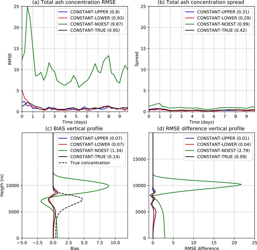
4                                                                                               S. Osores et al.: ETKF–FALL3D v1.0

Figure 1. Vertical mass distribution for different (a) eruptive column top heights and (b) A Suzuki parameters.

matrix estimated from the ensemble of forecasts:                        (e.g., cloud column mass load), and the vector  represents
             k                                                          the error in the observations. This error is typically assumed
 f                  f (i)
             X
s t = k −1         st       ,                                   (3)     to be a zero-mean Gaussian random variable with covariance
             i=1                                                        matrix R (dimensions of m × m). The errors in the observa-
                                                                        tions are assumed to be uncorrelated in time and indepen-
    f                   f fT
Pt = (k − 1)−1 St St ,                                          (4)     dent of the state of the system. Under these assumptions, the
                                                                        information provided by the forecast and the observations
         f                                       f
where s t is the ensemble forecast mean, Pt is the ensem-               can be combined to obtain an estimation of the augmented
ble forecast covariance matrix (a square matrix of dimension            state that minimizes the root mean square error (RMSE) with
                f
ns × ns ), and St is the ensemble forecast perturbation matrix          respect to the unknown truth (e.g., Kalnay, 2003; Carrassi
                                       f (i)
whose ith column is computed as St = st − st .
                                                f (i)   f (i)           et al., 2018):
    Note that the integration of the ensemble in time propa-                     f    f          f

                                                                                                                f         f

                                                                        s at = s t + Pt HTt (Ht Pt HTt + R)−1 y t − H(x t ) ,       (6)
gates the uncertainty on the initial conditions and parame-
ters at time t − 1 into the future in order to provide a time-
                                                                        where s at is the a posteriori estimation of the augmented state
dependent estimation of the forecast uncertainty. This is a
                                                                        (i.e., the analysis), and Ht is the tangent linear of the observa-
key feature that makes these methods particularly appealing                                            f         f
                                                                        tion operator. The factor Pt HTt (Ht Pt HTt + R)−1 is usually
for the estimation of uncertain model parameters (e.g., Aksoy
                                                                        referred to as the Kalman gain. The Kalman filter equations
et al., 2006; Ruiz et al., 2013) and for an accurate quantifi-
                                                                        also provide a way to estimate the uncertainty of the analy-
cation of concentration. At the analysis step a set of observa-
                                                                        sis. After the assimilation of the observations, the augmented
tions is available that is related to the true state of the system
                                                                        state covariance matrix is updated to
by the following expression:
                                                                                            f
y t = H x true

                 + t ,                                         (5)     Pat = (I − KHt )Pt ,                                          (7)
            t
where y t is an m-sized column vector containing the value of           where Patis the posterior or analysis-augmented state covari-
the m observations at time t, and x true is the true model state        ance matrix. Note that Eqs. (6) and (7) can be used to obtain
(assumed to be unknown). H is a (usually nonlinear) trans-              an ensemble of analyses for the state variables, and the pa-
                                                                                                                       f
formation that maps the state variables (i.e., ash concentra-           rameters whose ensemble mean is equal to s t and the pertur-
tions for different particle sizes) into the observed quantities        bations are sampled from a Gaussian distribution with zero

Geosci. Model Dev., 13, 1–22, 2020                                                              www.geosci-model-dev.net/13/1/2020/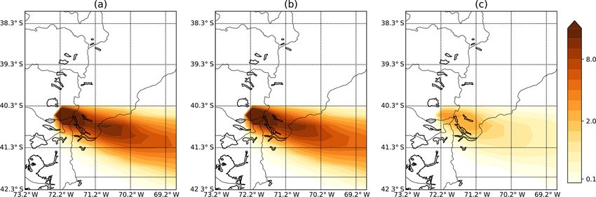
S. Osores et al.: ETKF–FALL3D v1.0 5
Table 1. Summary of the notation used in the paper, with the nomenclature for the ETKF method and its correspondence to the experiments
discussed in this work. Here, n is the total number of grid points times the number of particle classes in the FALL3D model, m is the number
of observations at time t, p is the number of parameters, and k is the number of ensemble members.
Nomenclature Dimension Description ETKF–FALL3D
Mt – Nonlinear model FALL3D model
y ot m×l Observations Satellite retrieval of ash mass loading
t m×1 Observational error Ash mass loading estimation error
f
xt n×k A priori or forecast ensemble Ensemble forecast of 3-D concentration
f
xt n×1 Background mean Mean of 3-D concentration short-term forecast
f
σt p×k A priori or forecast set of parameters A priori parameters ensemble used in the FALL3D
forecast
f
yt m×k Forecast into the observational space FALL3D ash mass loading ensemble forecast
f
yt m×1 Forecast mean Ash mass loading ensemble forecast mean
x at n×k A posteriori or analysis ensemble Ensemble analysis of 3-D concentration
x at n×1 Analysis mean Mean 3-D concentration analysis
σta p×k A posteriori or analysis set of parameters Ensemble of optimized set of parameters
Ht – Observational operator Transformation function from concentration to ash
mass loading
Ht m×n Tangent linear observation operator
f
Pt n×n Background error covariance matrix 3-D concentration forecast error covariance matrix
Pat n×n Analysis augmented state error covariance 3-D concentration analysis error covariance matrix
matrix
Rt m×m Observational error covariance matrix Ash mass loading error covariance matrix
f
st ns × 1 Augmented state vector Concatenation of the state vector x t and the esti-
f
mated model parameters σt
f
St ns × ns Ensemble forecast perturbation matrix
mean and covariance matrix equal to Pat . These equations ing they have a Gaussian distribution, k random samples are
can be difficult to solve explicitly for high-dimensional sys- taken. Each parameter sample is used in one of the ensemble
tems due to the large size of Pt and Rt , but several methods members integrated with the dispersion model. When an ob-
have been proposed to address this issue and to implement servation is available, it is combined with the ensemble fore-
the ensemble Kalman filter in high-dimensional systems. In casts using the ETKF equations. From this combination an
the present work, we use the ETKF approach, which solves ensemble of analysis is obtained with a set of optimized pa-
the ensemble Kalman filter equations in a subspace defined rameters that also has a Gaussian distribution. Then the next
by the ensemble members. Details about the equation that cycle starts from the ensemble of analysis and the set of opti-
arises from this particular implementation can be found in mized parameters to produce a new ensemble forecast. When
Hunt et al. (2007), but a summary is given in Appendix A. a new observation is available, the assimilation method is ap-
Table 1 also presents a summary of the notation and dimen- plied, and the cycle continues.
sions associated with the different quantities previously dis-
cussed. One of the main advantages of this approach is that
finding the analysis ensemble mean requires inverting a k ×k 3 ETKF–FALL3D experimental setup
matrix, which is significantly cheaper than inverting the n×n
matrix for the case in which k
n (which is usually the case To explore the capability of the ETKF–FALL3D system we
for high-dimensional applications of the filter). use an OSSE approach, in which a long model integration
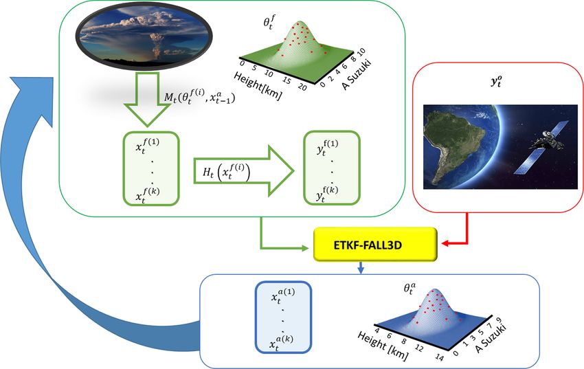
The process is schematically shown in Fig. 2. The cycle is performed and regarded as the true evolution of the ash
starts with an estimation of the mean parameters; assum- cloud. This model integration will be referred to as the nature
www.geosci-model-dev.net/13/1/2020/ Geosci. Model Dev., 13, 1–22, 2020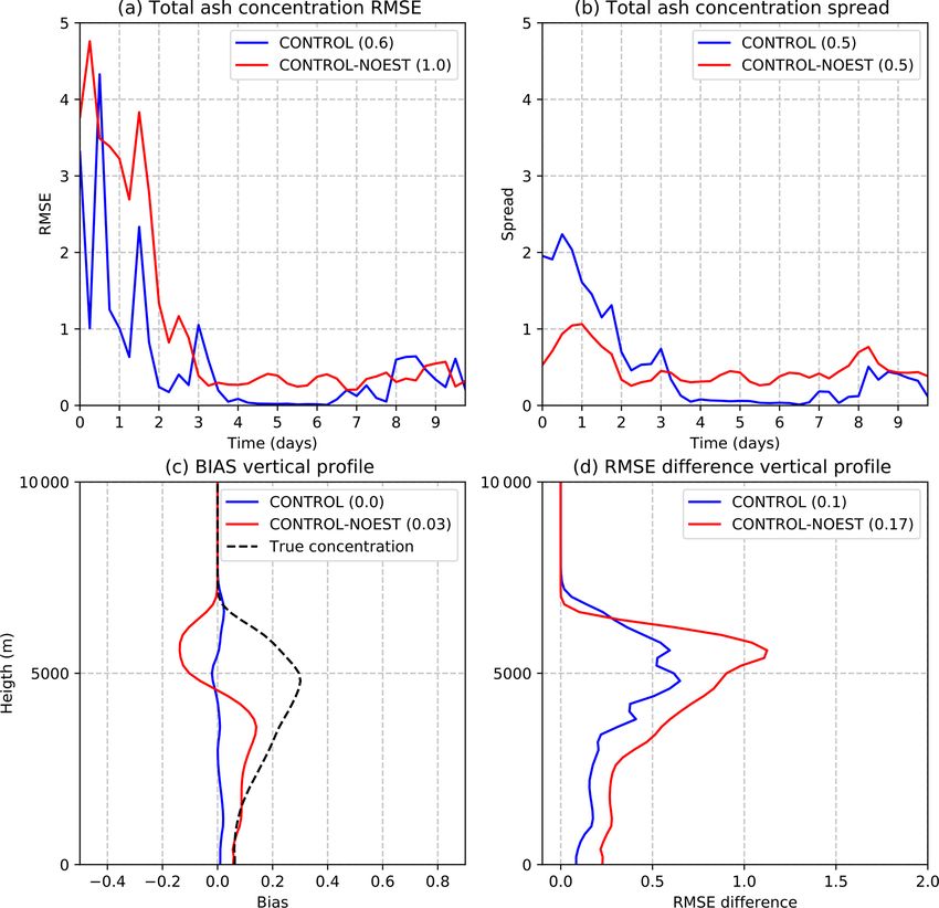
6 S. Osores et al.: ETKF–FALL3D v1.0
Figure 2. ETKF–FALL3D data assimilation system scheme for volcanic ash.
run. Observations are simulated from the nature run and then resolution of 0.5◦ , a temporal resolution of 6 h, and 27 con-
assimilated with the ETKF–FALL3D system. The June 2011 stant pressure vertical levels.
Puyehue-Cordón Caulle eruption (Osores et al., 2012; Collini The simulated observations represent ash mass column
et al., 2013) has been selected for the generation of the nature load (vertically integrated ash mass per unit area) estimates
run. retrieved from satellite radiances (e.g., Prata and Prata, 2012;
Francis et al., 2012; Pavolonis et al., 2013). Simulations of
3.1 Ash mass loading observation simulations satellite retrievals are chosen since these observations are
available almost globally and have a high spatial and tem-
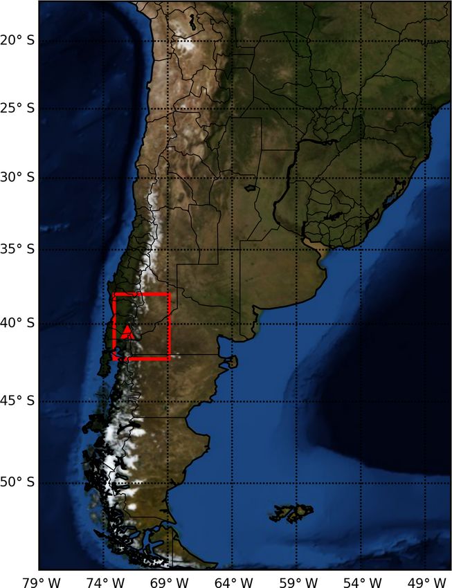
The nature run and observation simulation begin at poral resolution, making them particularly appealing for the
18:00 UTC on 4 June 2011 and last for 10 d up to 00:00 UTC implementation of operational data assimilation systems. To
on 15 June, covering the domain shown in Fig. 3 with a represent some of the limitations of current satellite-based
model horizontal resolution of 0.23◦ and a vertical resolu- ash mass load retrievals, the simulated observations are avail-
tion of 200 m. The model top is located at 20 km above the able only where the true load values are between 0.2 and
ground. The volcanic vent is located at 40.52◦ S–72.15◦ W at 10 g m−2 . The lower bound approximately corresponds to
an altitude of 1420 m a.s.l. the minimum mass load that can be retrieved by state-of-
The particle total grain size distribution (GSD) is repre- the-art algorithms. Retrievals usually cannot estimate mass
sented by 12 classes with diameters between 2 mm (−1φ) loads over the upper bound because the optical thickness of
and 1 µm (10φ) and densities ranging from 400 for the larger the corresponding ash plume is too high (e.g., Wen and Rose,
particles to 2100 kg m−3 for the smaller ones (Bonadonna 1994; Prata and Prata, 2012; Pavolonis et al., 2013). The ob-
et al., 2015). The vertical distribution of the source is param- servational error is assumed to have a random Gaussian dis-
eterized using the Suzuki scheme considering λ = 5, the set- tribution, with a standard deviation of 0.15 of the ash mass
tling velocity model is that of Ganser (Ganser, 1993), and the load.
vertical and horizontal turbulent diffusion are parameterized For the sake of simplicity, observations are assumed to be
by the similarity (Ulke, 2000) and Community Multiscale colocated with the model grid points; we also assume that
Air Quality (CMAQ) (Byun and Schere, 2006) schemes, re- observation errors are uncorrelated (i.e., R is diagonal) and
spectively. The meteorological fields are obtained from the that observations are unbiased. All observations are gener-
Global Forecasting System (GFS) analysis with a horizontal ated assuming a clear-sky condition both above and below
Geosci. Model Dev., 13, 1–22, 2020 www.geosci-model-dev.net/13/1/2020/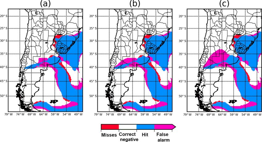
S. Osores et al.: ETKF–FALL3D v1.0                                                                                                  7

                                                                    Figure 4. Nature run parameter time series for the constant (solid
                                                                    lines) and variable emission profiles (dashed lines) for h (black
                                                                    lines) and A Suzuki (red lines).

                                                                    3.1.2    Variable emission profile

                                                                    In this experiment, h and A Suzuki are time-dependent
                                                                    (Fig. 4). In order to represent a realistic variability of the
                                                                    source parameters, the h evolution corresponds to the esti-
                                                                    mated heights during the 2011 Puyehue-Cordón Caulle erup-
                                                                    tion (Osores et al., 2014). Since the A Suzuki parameter can-
Figure 3. Domain used in the ETKF–FALL3D sensitivity tests (red     not be directly estimated, the evolution of this parameter is
square).                                                            simulated using an auto-regressive model (Fig. 4).
                                                                       In Fig. 5b and d, the ash mass loading fields for 7 June at
                                                                    12:00 UTC from the nature run and the observation simula-
the ash cloud. Two nature runs were generated to evaluate the       tion are shown. As has been shown for the constant parame-
ETKF–FALL3D system: one with constant emission profiles             ter case, the observational error does not significantly affect
and another with time-varying emission profiles.                    the spatial distribution of the plume. In this experiment, the
                                                                    number of observations assimilated depends on the emission
3.1.1   Constant emission profile
                                                                    profile as well as the wind field, and it can range from 15 (on
This nature run simulation considers a source term that re-         11 June at 06:00 UTC) to 86 (on 11 June at 18:00 UTC).
mains constant during the entire simulated period, with an
                                                                    3.2     Data assimilation experimental setup
eruption column height of 8.5 km above the vent and an A
Suzuki parameter of 5.5 (Fig. 4). Figure 5a and c show the          In the data assimilation experiments performed in this work,
ash mass loading from the nature run and the observation            the simulated observations are assimilated every 6 h. The
simulation on 7 June at 12:00 UTC for illustrative purposes.        number of ensemble members in the experiments is set to
The addition of observational error to the nature run does          32 (unless stated otherwise). In most experiments source pa-
not significantly affect the spatial distribution or the location   rameters are assumed to be unknown and estimated within
and intensity of the maximum concentration. The number of           the data assimilation cycle. The model grid, boundary condi-
available observations (which depends on the thresholds de-         tions, and all other model parameters and configuration op-
scribed in the previous section) is time-dependent (ranging         tions are set as in the nature run. The ensemble at the first
from 27 to 52 grid point observations) and, in this partic-         assimilation cycle is initialized using zero ash concentrations
ular case, is primarily affected by the atmospheric circula-        for all members and a set of parameters that are sampled ran-
tion, which produces variations in the 3-D ash concentration        domly from a Gaussian distribution whose mean and vari-
within the model domain.                                            ance for each experiment are detailed below. The relaxation
                                                                    to prior spread (RTPS; Whitaker and Hamill, 2012) inflation
                                                                    approach, with a parameter of α = 0.5, is applied to the state
                                                                    variables to reduce the impact of sampling error. For the pa-

www.geosci-model-dev.net/13/1/2020/                                                           Geosci. Model Dev., 13, 1–22, 2020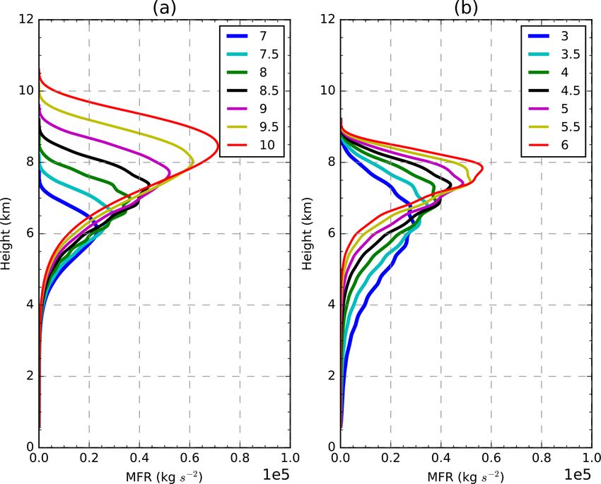
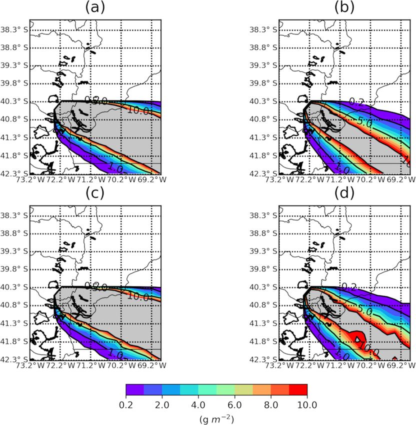
8                                                                                           S. Osores et al.: ETKF–FALL3D v1.0

Figure 5. Ash mass loading on 7 June at 12:00 UTC for (a) the nature run with constant parameters, (c) the run with observational error
and constant parameters, the (b) nature run with time-dependent parameters, and (d) the run with observational error and time-dependent
parameters. Ash mass loading values outside the 0.2–10.0 g m−2 interval are in grey.

rameters, the ensemble spread is inflated back to its origi-          domains, using covariance localization will highly improve
nal value after assimilating the observations (similar to the         its performance.
conditional inflation approach of Aksoy et al., 2006). This              Given that in the ensemble Kalman filter the distribution
is equivalent to assuming that the parameter uncertainty is           of ash concentration and parameters is assumed to be Gaus-
time-independent, thus preventing the parameter ensemble              sian, a negative ash concentration or nonphysical parame-
spread from collapsing. Covariance localization is usually            ter values can result from the assimilation of observations.
required to reduce the impact of spurious correlation that re-        These nonphysical solutions must be corrected before using
sults from the use of small ensemble sizes. The estimation of         the analysis ensemble as initial conditions for the next en-
small correlations (e.g., between locations that are far apart        semble forecast cycle. For ash concentration, negative values
from each other) is usually strongly affected by sampling             are turned into zero concentrations. In the case of eruption
noise; this is why estimated covariances are usually forced           source parameters, nonphysical values are checked individu-
to decay with distance. Since the domain used in the data as-         ally for each ensemble member and replaced with a random
similation experiments is small, the impact of spurious corre-        realization from a Gaussian distribution with the same mean
lations between distant grid points is less significant. For this     and standard deviation as the analysis ensemble. If the ran-
reason, no covariance localization is used in the estimation          domly generated value is outside the physically meaningful
of the state variables or the parameters. However, is impor-          range for the parameter, the process is repeated until the ran-
tant to keep in mind that if the system is extended to larger         domly generated value is within the physically meaningful

Geosci. Model Dev., 13, 1–22, 2020                                                          www.geosci-model-dev.net/13/1/2020/
S. Osores et al.: ETKF–FALL3D v1.0 9
range. The physically meaningful range for model parame- To explore the impact of modifying the ensemble size, an
ters is set to 0–20 km and 0–15 for h and A Suzuki, respec- experiment with ensemble sizes of 8 (ENS-8) and 16 (ENS-
tively. The number of grid points and ensemble members 16) is presented for which all other configuration settings are
with estimated concentrations below −1.0 × 10⁻⁴ g m−3 is equal to the CONTROL run experiment. Finally, the impact
usually below 15 % of the grid points and ensemble mem- of observation error is assessed in two experiments with ob-
bers for which the concentration has been updated. This pro- servation errors that are 30 (OBS-30) and 40 % (OBS-40) of
portion decreased with increasing ash concentration as well the true total mass concentration. All presented data assimi-
as with ensemble spread. Estimated parameters for individ- lation and parameter estimation experiments are summarized
ual ensemble members fall outside the physical meaningful in Table 2, including the statistical properties of the initial
range less than 10 % of the times, also depending on how parameter ensemble. Finally, a set of simulation experiments
close to the boundaries the true parameters are and how large is carried out using a larger domain to evaluate the impact
the parameter ensemble spread is. of the optimized parameters upon the simulation of the ash
One of the main hypotheses of the Kalman filter is that cloud farther from the vent.
state variables and parameters are approximately linearly
correlated with the observations. This is not true for the h 3.3 Performance metrics
parameter since in the Mastin et al. (2009) emission scheme
the source strength is proportional to the fourth power of h. The evaluation of the FALL3D-ETKF system is achieved by
For this reason, instead of estimating h, we estimate h4 so comparing the 3-D ash concentration forecast (and analysis)
that the estimated parameter is more linearly correlated with against the nature run and also by measuring the consistency
the observations. between the estimated and the actual forecast uncertainties.
In this work, several experiments are performed to study The comparison is based on the RMSE, error bias, and the
the convergence of the filter and its sensitivity to some key ensemble spread of either the forecast or the analysis, which
parameters. Two experiments are performed using the con- are given by the following expressions:
stant parameter nature run to assess filter convergence. The v
N
u
first experiment starts with source parameters that are higher u X 2
than the true value and will be referred to as CONSTANT- RMSE = tN −1 x f,i − x t,i , (8)
i=1
UPPER; the second starts with an underestimation of the
N
source parameters and will be referred to as CONSTANT- X
BIAS = N −1
LOWER. The initial parameter spread for h and A Suzuki x f,i − x t,i , (9)
i=1
is 500 and 0.5 m, respectively, and is the same for both ex- v !
periments. These experiments are compared against an ex-
u N k 2
(j )
u X X
periment in which parameters remain constant at their initial SPREAD = tN −1 k −1 x f ,i − x f,i , (10)
value (CONSTANT-NOEST) and against an experiment in i=1 j =1
which the parameters are constant and their ensemble mean
where x f,i is either the forecast or analysis ensemble mean
is equal to the true value (CONSTANT-TRUE). (j )
The second set of experiments is based on the nature run ash concentration at time and location i and x f,i , and x t,i
with time-dependent parameters. An estimation experiment represents their corresponding values for the j th ensemble
that uses the same parameter ensemble spread as in the pre- member and the nature run, respectively. Spatial or temporal
vious experiments is performed and will be referred to as averages are obtain by summing over i.
the CONTROL experiment. To evaluate the impact of per-
forming parameter estimation in the time-dependent param- 4 Results
eter context, an experiment in which the parameters are kept
constant at the time average of the true parameters is also 4.1 Constant emission profile experiments
presented (CONTROL-NOEST).
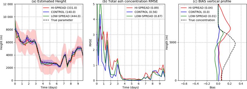
To quantify the sensitivity of the ETKF–FALL3D system In these experiments, we explore the impact of data assimi-
to the parameter ensemble spread, two additional experi- lation and parameter estimation in the steady parameter sce-
ments are performed: one in which the ensemble spread is nario. Figure 6 shows the ensemble mean and the spread of
larger than in the CONTROL experiment (HI-SPREAD), for h and A Suzuki. After the first assimilation cycle, both pa-
which the spread in h and A Suzuki is 2000 and 4 m, respec- rameters start to converge rapidly to values close to the true
tively, and another experiment in which the ensemble spread ones, with mean errors below 500 and 1 m, respectively. The
is lower than in the CONTROL run (LOW-SPREAD), for convergence of h is faster, likely due to the strongest sensitiv-
which the spread in h and A Suzuki is 100 and 0.1 m, re- ity of forecasted ash concentrations to column height in the
spectively. All the other configuration settings are as in the surroundings of the source. The two experiments consider-
CONTROL experiment. ing different initial parameter values (CONSTANT-UPPER
and CONSTANT-LOWER) converge to values close to the
www.geosci-model-dev.net/13/1/2020/ Geosci. Model Dev., 13, 1–22, 2020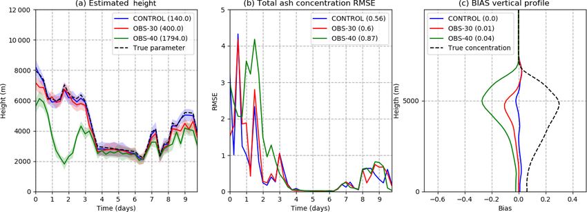
10                                                                                             S. Osores et al.: ETKF–FALL3D v1.0

Table 2. Summary of the main parameters that distinguish the different experiments described in the text.

             Name                      Ens. size   h ini. (m)   A ini.   h spread (m)    A spread    Par. est.   Obs. err. (%)
             CONSTANT-UPPER                  32       11.000      7.0           500.0          2.0          y              15
             CONSTANT-LOWER                  32        3.000      2.0           500.0          2.0          y              15
             CONSTANT-NOEST                  32        3.000      2.0           500.0          2.0          n              15
             CONSTANT-TRUE                   32        8.500      5.5           500.0          2.0          n              15
             CONTROL                         32       11.000      7.0           500.0          2.0          y              15
             CONTROL-NOEST                   32       11.000      7.0           500.0          2.0          n              15
             HI-SPREAD                       32       11.000      7.0          2000.0          4.0          y              15
             LOW-SPREAD                      32       11.000      7.0           100.0          0.1          y              15
             ENS-16                          16       11.000      7.0           500.0          2.0          y              15
             ENS-8                            8       11.000      7.0           500.0          2.0          y              15
             OBS-30                          32       11.000      7.0           500.0          2.0          y              30
             OBS-40                          32       11.000      7.0           500.0          2.0          y              40

Figure 6. Optimized parameters as a function of time in the CONSTANT-UPPER (blue line), CONSTANT-LOWER (red line), CONSTANT-
TRUE (black line), and CONSTANT-NOEST (green line) experiments. The shading surrounding the CONSTANT-UPPER and CONSTANT-
LOWER estimated values represents ± 1 standard deviation; (a) h parameter and (b) A Suzuki parameter.

true parameter, indicating that the parameter estimation tech-              Figure 7a shows the time evolution of the domain-
nique is robust in finding the correct values of parameters              averaged RMSE for the 3-D total ash concentration forecasts.
regardless of ensemble initialization. As observed in Fig. 6,            The RMSE of the parameter estimation experiments is com-
both parameter estimation experiments tend to sub-estimate               pared against an experiment in which parameters are not es-
the values of h and to slightly overestimate the values of A             timated and are fixed at the initial value of the CONSTANT-
Suzuki. Figure 6 also shows the parameter ensemble spread.               UPPER experiment (CONSTANT-NOEST) and against an
In these experiments, the ensemble almost always contains                experiment in which the parameter ensemble is centered
the true parameter value, meaning that the parameter uncer-              at the true value of the source parameters (CONSTANT-
tainty is well captured by the ensemble. However, it should              TRUE). Parameter estimation experiments show similar re-
be noted that, in these experiments, the ensemble spread of              sults in terms of the 6 h forecast errors, indicating the ro-
the model parameters is prescribed a priori to a value that              bustness of the convergence to the optimal parameter val-
may not be the optimal one under different conditions (e.g., if          ues. Moreover, both parameter estimation experiments show
the optimal parameters are time-dependent or if other sources            ash concentration errors that are similar to the one obtained
of uncertainty, like errors in the atmospheric circulation, are          in the CONSTANT-TRUE experiment and are much lower
present). Sensitivity experiments to the parameter ensemble              than the errors obtained in the CONSTANT-NOEST exper-
spread will be discussed in the following sections.                      iment, clearly showing the advantage of performing data-
                                                                         assimilation-based source parameter estimation. Figure 7b

Geosci. Model Dev., 13, 1–22, 2020                                                             www.geosci-model-dev.net/13/1/2020/
S. Osores et al.: ETKF–FALL3D v1.0 11 shows the spatially averaged ash concentration ensemble concentrations and mass loadings are obtained by taking into spread. One way to assess if the current parameter ensemble account the uncertainties associated with the source parame- spread is well tuned is to compare the ash concentration fore- ters. cast error and spread. If these are similar then we can assume that our uncertainty is well represented in the ensemble. In 4.2 Time-dependent emission experiments this case, the uncertainty in the ash concentration is mainly associated with the uncertainty in the source parameters. As These experiments use the observations simulated from the observed, the spread values are close to the RMSE values in nature run with time-varying parameters (Fig. 4). The pa- Fig. 7a, which indicates that after convergence of the param- rameter ensemble is initialized with a mean h of 11 km, a eters, the ensemble spread closely represents the magnitude mean A Suzuki of 7, and standard deviations of 0.5 and of the errors. 2.0 km, respectively. Figure 8 shows the evolution in time Figure 7c shows the horizontal and time-averaged error of the optimized parameter ensemble as well as their corre- bias for the total ash concentration as a function of height. sponding true values, showing a good agreement. The esti- The first 2 d have been excluded because they are considered mation of h seems to be particularly accurate and can detect part of the spin-up time of the filter. This figure shows that rapid variations in the eruptive column height, with RMSE biases associated with the estimation experiments are much values lower than 200 m throughout the experiment. For the lower than for the CONSTANT-NOEST experiment, show- A Suzuki parameter, the time evolution is not reproduced so ing once again the advantage of optimizing the source pa- accurately. There are also two sudden jumps in the estima- rameters. The CONSTANT-UPPER, CONSTANT-LOWER, tion of A Suzuki, indicating a less well-constrained parame- and CONSTANT-TRUE experiments show a small system- ter value. These differences in the behavior of the estimated atic underestimation of the maximum concentrations and an h and A Suzuki may be due to the higher sensitivity of the overestimation above and below the location of the maxi- ash distribution to the eruptive column height in comparison mum. Note that the bias is slightly lower in the parameter es- with the A Suzuki parameter. The jumps in the estimated A timation experiments with respect to the CONSTANT-TRUE Suzuki occur during periods of fast changes in h, suggesting experiment. that when h is not well estimated, A Suzuki may be modified The fact that a biased parameter ensemble (i.e., the under- in an attempt to compensate for errors in h. estimation of h observed in Fig. 6a) produces a less biased es- Figure 9 shows the RMSE of the forecast for the 3-D to- timation of ash concentrations (Fig. 7c) may be related to the tal ash concentration. Errors in this case vary strongly with nonlinear relationship between h and the total mass emission time, with larger errors corresponding to the instants in which at the source. Since the emitted mass depends on h4 , positive h is larger, leading to stronger ash mass emission at the vent perturbations in h are associated with a much larger emission and consequently larger ash concentrations in the surround- rate and are thus farther from the observations than ensem- ings of the vent. The ensemble spread (Fig. 9b), although ble members with negative perturbations in h. This creates a smaller than the error (indicating an under-dispersive ensem- bias in the estimation of the concentrations because, even if ble), changes accordingly with more spread during the peri- the ensemble is centered at the true h value, positive pertur- ods in which the emission is higher. These changes in the en- bations are farther from observations than the negative ones, semble spread are a consequence of the relationship between and therefore the ensemble mean tends to overestimate con- h and mass emission at the vent. Since h deviations from the centrations. ETKF tries to compensate for this effect by con- ensemble mean are almost time-independent, the associated verging to a slightly biased parameter set, which reduces the departures in mass emission are larger during the periods of error bias and the RMSE. higher h, leading to a larger spread in the concentration field. As observed in Fig. 7d, the analysis error in ash concentra- Figure 9d shows the spatially averaged reduction in the tion is below the forecast error. This indicates that the ETKF RMSE for the total ash concentration between the forecast method is efficient in reducing the error in the 3-D concentra- and the analysis. The RMSE is reduced between the forecast tion field based on the information provided by a 2-D obser- and the analysis at almost all vertical levels, indicating that vation. This is a remarkable result in a context in which most the vertical covariance structure between mass loadings and observations are 2-D, whereas operational requirements are ash concentrations at different levels is well estimated, lead- 3-D. This finding will be the basis for using the analysis as a ing to accurate 3-D ash concentration estimations. better diagnostic of the state of the plume to improve the fore- In order to assess the impact of treating the parameters casts. The reason behind this lies in the structure of the fore- as a time-dependent variable, this experiment is compared cast error covariance matrix, which is estimated from the en- with an experiment in which data assimilation is performed semble of forecasts. This matrix contains information about but only the ash concentration field is updated. In this case, the covariances between mass loading (which is the observ- source parameters are kept constant in time at a value equal able quantity) and the concentration at different heights from to the time average of the true parameters (CONTROL- which the mass loading is obtained and which are not directly NOEST, Fig. 8). This value is chosen to obtain a solution observed. In this work, reliable covariances between 3-D ash that is as close as possible to the one obtained with the www.geosci-model-dev.net/13/1/2020/ Geosci. Model Dev., 13, 1–22, 2020
12                                                                                             S. Osores et al.: ETKF–FALL3D v1.0

Figure 7. (a) Spatially averaged forecasted total ash concentration RMSE, (b) spatially averaged forecasted total ash concentration ensemble
spread, (c) spatially averaged forecasted total ash concentration bias, and (d) the difference between the 6 h forecast and analysis total
ash concentration RMSE for the CONSTANT-UPPER (blue line), CONSTANT-LOWER (red line), CONSTANT-TRUE (black line), and
CONSTANT-NOEST (green line) experiments. Panels (a), (b), and (c) are computed from the 6 h ensemble forecast (all values: 10−3 g m−3 ).

time-dependent parameters. Figure 9 shows that the forecast             similation for the estimation of 3-D ash concentrations is not
RMSE and bias in the 3-D ash concentration are almost al-               sufficient to properly constrain 3-D ash concentration val-
ways larger in the CONTROL-NOEST experiment with re-                    ues and that source parameters also have to be taken into ac-
spect to the CONTROL experiment. The error in the CON-                  count, particularly close to the source where these parameters
TROL and CONTROL-NOEST experiments becomes simi-                        rapidly impact concentrations.
lar around day 3 and after day 8 because at those times in-                As an example, Fig. 10 shows the ensemble forecast mean
stants the source parameters are close to each other (Fig. 8).          for the CONTROL and CONTROL-NOEST experiments
Moreover, the ensemble spread for the CONTROL-NOEST                     and the nature run at FL200 at the 12th assimilation cy-
experiment is almost constant in time and, because of that,             cle. The ash concentration pattern at this particular level is
changes in the forecast uncertainty are not captured (Fig. 9b).         well represented by the simulation that estimates the source
This is because time variations in the ensemble spread are              parameters, whereas in the CONTROL-NOEST experiment,
mainly associated with changes in the mean values of pa-                there is a significant underestimation of the concentrations
rameters. These experiments suggest that performing data as-            due to the underestimation of the column height at this par-

Geosci. Model Dev., 13, 1–22, 2020                                                              www.geosci-model-dev.net/13/1/2020/
S. Osores et al.: ETKF–FALL3D v1.0                                                                                                 13

Figure 8. Optimized parameters as a function of time in the CONTROL (blue line) and CONTROL-NOEST (red line) experiments. The
shading surrounding the estimated values represents ± 1 standard deviation; (a) h parameter and (b) A Suzuki parameter. The black line
indicates the value of the parameters in the true run.

ticular time. Note that data assimilation is being performed         periment. Slower convergence or a lack of convergence is
to correct the 3-D ash concentrations in both experiments.           expected when the parameter uncertainty is underestimated.
                                                                     In this case, the ETKF does not allow for large corrections
4.3   Sensitivity experiments                                        in the parameter values based on the observations, basically
                                                                     because the error in the parameters is assumed to be small.
This section discusses the sensitivity of the analysis and the       These experiments show that the system is particularly sensi-
forecast to the parameter ensemble spread, the ensemble size,        tive to the parameter ensemble spread that has to be specified
and the observation uncertainty. The purpose is to identify          a priori. Moreover, in these idealized experiments, the opti-
the potentially more important tuning parameters for the op-         mal parameter ensemble spread is determined by the uncer-
timization of the system and how robust the system is with           tainty in the observations and with no information regarding
respect to errors in observations, which are known to exist in       the changes in the true parameters in time.
satellite-based ash mass loading estimations.                           As discussed in Sect. 4.1, parameters are estimated based
   To explore the sensitivity to the parameter ensemble              on their covariance with the observed quantities. In the
spread, the experiments CONTROL, HI-SPREAD, and                      ensemble-based data assimilation methods, these covari-
LOW-SPREAD with different parameter spreads (Table 2)                ances are estimated directly from the ensemble, so they can
are compared. Figure 11 shows the estimated h obtained               be affected by sampling errors. To assess the impact of these
in these experiments as well as the total ash concentration          sampling errors on the analysis, quality assimilation exper-
RMSE and bias. As observed, the CONTROL experiment                   iments with different ensemble sizes have been performed.
gives a more accurate estimation of h and the minimum                Three experiments with 8, 16, and 32 ensemble members are
RMSE and bias. When the parameter ensemble spread is                 presented (ENS-8, ENS-16, and CONTROL, respectively).
larger than in the CONTROL experiment, parameter values              Figure 12 shows the results in terms of h estimation and total
are systematically underestimated. As previously discussed,          ash concentration RMSE and bias. The CONTROL experi-
this can be explained by the nonlinear dependence between            ment shows a more accurate h estimation and consistently
h and the total emitted mass. However, what is relevant from         lower RMSE and bias values. However, the results are not
this experiment is that increasing the ensemble spread de-           very sensitive to the size of the ensemble. The lack of sen-
grades the quality of the estimation and increases the im-           sitivity to the ensemble size might be surprising, particularly
pact of nonlinearities. Higher dispersion in h increases the         considering that no spatial localization is being used in order
magnitude of positive h perturbations, leading to a larger           to reduce the impact of sampling errors. However, note that in
error bias, particularly above and below the maximum con-            this case, the only source of uncertainty in the system comes
centration (Fig. 11c). In the case of the LOW-SPREAD ex-             from the uncertain parameters. Based on this, uncertainties
periment, results are closer to the CONTROL experiment.              have to be constrained in two dimensions. This is confirmed
However, this experiment shows a slower convergence with             by the strong covariances that exist between the parameters
larger h estimation errors during the first days of the ex-          and ash concentration within the domain (not shown). This

www.geosci-model-dev.net/13/1/2020/                                                            Geosci. Model Dev., 13, 1–22, 2020
14 S. Osores et al.: ETKF–FALL3D v1.0 Figure 9. As in Fig. 7 but for the experiments CONTROL (blue line) and CONTROL-NOEST (red line; all values: 10−3 g m−3 ). effective low dimensionality is reinforced by the fact that the expected, the best results are obtained with the lowest ob- domain is small and close to the source, and, because of that, servation error. However, one interesting result is that as the the ash concentration at most grid points is strongly corre- observation error increases, estimated h values are lower, lated with the value of the uncertain source parameters. eventually leading to substantial underestimations such as the The last sensitivity experiment looks into the issue of ob- ones seen for OBS-40 during the first days of the experiment. servation errors in satellite retrievals of mass loadings. In the Moreover, this systematic underestimation of h produces an experiments presented so far, the standard deviation of the underestimation of the total ash concentrations, as is visible observation errors has been assumed to be 15 % of the mass in the bias profiles (Fig. 13c). Under the hypothesis of the loading in the nature run. However, in real cases, uncertain- ensemble Kalman filter, an increase in the observation error ties associated with mass loading estimations can be larger leads to an increase in the RMSE of the estimation. How- than that. Two additional experiments are performed to ex- ever, in this case, the systematic component of the error is plore the impact of the magnitude of the observation errors also increased. This behavior is probably a consequence of on the estimation of source parameters and total ash con- the nonlinear effects arising from the nonlinear relationship centrations with an observation standard deviation of 30 % between h and the ash emission rate that has been previously (OBS-30) and 40 % (OBS-40) of the true mass loading value. discussed. Results from these experiments are presented in Fig. 13. As Geosci. Model Dev., 13, 1–22, 2020 www.geosci-model-dev.net/13/1/2020/
S. Osores et al.: ETKF–FALL3D v1.0                                                                                                             15

Figure 10. (a) Nature run ash concentration at flight level 200 (shaded, 10−3 g m−3 ); (b) as in (a) but for the 6 h forecast of ash concentration
initialized from the CONTROL analysis experiment; (c) as in (b) but for the CONTROL-NOEST experiment, corresponding to the 12th
assimilation cycle.

Figure 11. (a) Estimated h as a function of time for the HI-SPREAD (red line), CONTROL (blue line), and LOW-SPREAD (green line). The
shading surrounding the estimated values represents ± 1 standard deviation, and the black dashed line indicates the true parameter value.
(b) Spatially averaged total ash concentration 6 h forecast RMSE as a function of time (10−3 g m−3 ). Line color code as in (a). (c) Temporally
averaged 6 h forecast bias as a function of height (10−3 g m−3 ). Line color code as in (a).

4.4   Ash concentration simulations in an extended                            To see if the estimated parameters can be used to recon-
      domain simulation                                                    struct the ash cloud far from the source, the estimated param-
                                                                           eters are used to produce a simulation of the ash cloud over
The experiments discussed so far have been performed in a                  a larger domain. At each time the source parameter values
relatively small domain surrounding the vent. In most appli-               in this simulation are taken from the CONTROL run param-
cations, however, it is expected that forecasts over larger do-            eter ensemble mean. This simulation will be referred to as
mains are required. In this section, we explore the adequacy               CONTROL-LD. Figure 14a shows the results of comparing
of the parameter estimation approach to generate a good esti-              the ash mass loading above 0.2 g m−2 from the experiment
mation of ash dispersion over larger domains in an idealized               forced with the estimated parameters against the nature run.
context in which the atmospheric flow is perfectly known.                  The comparison of these categorical variables shows that hits
For this purpose, a nature simulation over a larger domain                 (i.e., grid points in which mass loadings are over the selected
is performed. This nature run is forced with the same evo-                 threshold for both the simulation and the nature run) prevail,
lution as parameters of the time-dependent parameter nature                with a lower number of false alarms and misses (i.e., grid
run and spanning the same period.                                          points in which the simulation is over the threshold and the

www.geosci-model-dev.net/13/1/2020/                                                                    Geosci. Model Dev., 13, 1–22, 2020
You can also read