Seasonal forecasts of the Saharan heat low characteristics: a multi-model assessment
←
→
Page content transcription
If your browser does not render page correctly, please read the page content below
Weather Clim. Dynam., 2, 893–912, 2021
https://doi.org/10.5194/wcd-2-893-2021
© Author(s) 2021. This work is distributed under
the Creative Commons Attribution 4.0 License.

Seasonal forecasts of the Saharan heat low characteristics:
a multi-model assessment
Cedric G. Ngoungue Langue1,4 , Christophe Lavaysse4,5 , Mathieu Vrac2 , Philippe Peyrillé3 , and Cyrille Flamant1
1 Laboratoire Atmosphères, Milieux, Observations Spatiales (LATMOS) – UMR 8190 CNRS–Sorbonne Université–UVSQ,
78280 Guyancourt, France
2 Laboratoire des Sciences du Climat et de l’Environnement, CEA Paris-Saclay l’Orme des Merisiers, UMR 8212

CEA–CNRS–UVSQ, Université Paris-Saclay & IPSL, 91191 Gif-sur-Yvette, France
3 Centre National de Recherches Météorologiques (CNRM) – Université de Toulouse, Météo-France,

CNRS, 31057 Toulouse CEDEX 1, France
4 Université Grenoble Alpes, CNRS, IRD, G-INP, IGE, 38000 Grenoble, France
5 European Commission, Joint Research Centre (JRC), 21027 Ispra, VA, Italy

Correspondence: Cedric G. Ngoungue Langue (cedric-gacial.ngoungue-langue@latmos.ipsl.fr)

Received: 14 April 2021 – Discussion started: 26 April 2021
Revised: 23 July 2021 – Accepted: 2 August 2021 – Published: 15 September 2021

Abstract. The Saharan heat low (SHL) is a key component of        yearly distribution of the SHL and the forecast scores. The
the West African Monsoon system at the synoptic scale and         results highlight the capacity of the models to represent the
a driver of summertime precipitation over the Sahel region.       intraseasonal pulsations (the so-called east–west phases) of
Therefore, accurate seasonal precipitation forecasts rely in      the SHL. We notice an overestimation of the occurrence of
part on a proper representation of the SHL characteristics in     the SHL east phases in the models (SEAS5, MF7), while
seasonal forecast models. This is investigated using the latest   the SHL west phases are much better represented in MF7. In
versions of two seasonal forecast systems namely the SEAS5        spite of an improvement in prediction score, the SHL-related
and MF7 systems from the European Center of Medium-               forecast skills of the seasonal forecast models remain weak
Range Weather Forecasts (ECMWF) and Météo-France re-              for specific variations for lead times beyond 1 month, requir-
spectively. The SHL characteristics in the seasonal forecast      ing some adaptations. Moreover, the models show predictive
models are assessed based on a comparison with the fifth          skills at an intraseasonal timescale for shorter lead times.
ECMWF Reanalysis (ERA5) for the period 1993–2016. The
analysis of the modes of variability shows that the seasonal
forecast models have issues with the timing and the intensity
of the SHL pulsations when compared to ERA5. SEAS5 and            1   Introduction
MF7 show a cool bias centered on the Sahara and a warm
bias located in the eastern part of the Sahara respectively.      In the Sahel region, food security for populations depends on
Both models tend to underestimate the interannual variabil-       rainfed agriculture which is conditioned by seasonal rainfall
ity in the SHL. Large discrepancies are found in the repre-       (Durand, 1977; Bickle et al., 2020), characterized by a strong
sentation of extremes SHL events in the seasonal forecast         convective activity in the summer, associated with a large
models. These results are not linked to our choice of ERA5        climatic variability (local- and large-scale forcings), gener-
as a reference, for we show robust coherence and high cor-        ally leading to poor precipitation forecast skills at subsea-
relation between ERA5 and the Modern-Era Retrospective            sonal and seasonal timescales in tropical North Africa (Vo-
analysis for Research and Applications (MERRA). The use           gel et al., 2018). Hence, climate models suffer from biases
of statistical bias correction methods significantly reduces      in the representation of West African Monsoon (WAM) pro-
the bias in the seasonal forecast models and improves the         cesses and dynamics responsible for rainfall in West Africa
                                                                  (Roehrig et al., 2013; Martin et al., 2017). During the African

Published by Copernicus Publications on behalf of the European Geosciences Union.
894                              C. G. Ngoungue Langue et al.: Seasonal forecasts of the Saharan heat low characteristics

Monsoon Multidisciplinary Analysis (AMMA) project (Re-             posed into two phases called east–west oscillations. The west
delsperger et al., 2006), the Saharan heat low (SHL) has           phase corresponds to a maximum temperature over the coast
been used as a key component to assess the variability in the      of Morocco–Mauritania, propagating southwestward, and a
WAM system. In particular, forecasters and researchers have        minimum temperature between Libya and Sicily, propagat-
pointed out the need to document the SHL predictability and        ing southeastward. The east phase corresponds to the oppo-
its link with Sahelian rainfall (Janicot et al., 2008b). Improv-   site temperature structure which propagates as in the west
ing precipitation forecasts not only is crucial for agriculture    phase. Roehrig et al. (2011) studied the link between the vari-
and water supply in the region but also is of paramount im-        ability in convection in the Sahel region and the variability
portance for floods and disease prevention.                        in the SHL at an intraseasonal timescale using NCEP-2 re-
   The SHL refers to the low-surface-pressure area that ap-        analysis data. They showed that the onset of the monsoon
pears above the Sahara region in the boreal summer due             is associated with strong SHL activity when the northerlies
to seasonal high temperatures and insolation (e.g., Lavaysse       coming from the Mediterranean (sometimes called ventila-
et al., 2009). The SHL is an essential component of the WAM        tion) are weak. Conversely, they revealed that the formation
system at the synoptic scale (Sultan and Janicot, 2003; Parker     of a strong cold air surge over Libya and Egypt and its prop-
et al., 2005; Peyrillé and Lafore, 2007; Lavaysse et al., 2009;    agation toward the Sahel lead to the decrease in the SHL,
Chauvin et al., 2010) and a driver of precipitation over the       which inhibits the WAM onset.
Sahel region (Lavaysse et al., 2010a; Evan et al., 2015). It          As detailed above, previous work has evidenced the im-
plays an important role in the atmospheric circulation over        portance and the role of the SHL in the West African climate.
West Africa and brings moisture from the Atlantic Ocean to         These studies are based on a climatological view of the SHL
the region, thereby favoring the installation of the monsoon       using mostly reanalysis data. One may legitimately wonder
flow. In the lower atmospheric layers, the cyclonic circulation    how seasonal forecast models represent the SHL evolution.
generated by a strong SHL tends to reinforce the monsoon              The seasonal forecast is a long-term forecast which is very
flow around its eastern flank and the Harmattan flow along         useful because it allows an anticipation of seasonal trends.
the western flank (Lavaysse, 2015). In the mid-layers, the         The use of an ensemble forecast for seasonal forecasting pro-
anticyclonic circulation associated with the divergent flow at     vides a range of forecasts and gives information about the
the top of the SHL contributes to maintaining the African          spread associated with the forecast of a specific variable. En-
Easterly Jet (AEJ) at around 700 hPa and modulates its in-         semble forecast models lead to an improvement in the pre-
tensity (Thorncroft and Blackburn, 1999). An intensification       dictive skills of some atmospheric variables (Haiden et al.,
of the AEJ is observed during strong phases of SHL activity        2015; Lavaysse et al., 2019). The evaluation of the SHL be-
(Lavaysse et al., 2010b). According to Lavaysse et al. (2009),     havior in seasonal forecast models has not been addressed
the SHL maximum activity over the Sahara occurs on av-             yet. Roehrig et al. (2013) show that the mean temperature
erage from 20 June to 17 September, and it is located 20–          over the Sahara from July to September is well correlated
30◦ N, 7◦ W–5◦ E, covering much of northern Mauritania,            with rainfall position over the Sahel region. Provided that the
Mali, Niger and southern Algeria (Fig. 1). The maximum of          SHL characteristics (i.e., the east and west pulsations of the
SHL activity happens during the rainfall season in the Sahel       heat low, its intensity, and its interannual variability) are well
region (from June to September; Sultan and Janicot, 2003).         captured in seasonal forecast models simulations, they can
The SHL is considered a reliable proxy for the regional- and       be used as predictors for rainfall in the Sahel area.
large-scale forcings impacting the WAM (Lavaysse et al.,              The goal of this article is (i) to investigate the representa-
2010b).                                                            tion and the forecast skills of the SHL in two seasonal fore-
   Lavaysse et al. (2009) monitored the seasonal evolution of      cast models and (ii) to evaluate the added value of bias cor-
the West African heat low (WAHL) using ERA-40 reanaly-             rection techniques on raw seasonal forecasts. Bias issues are
ses and brightness temperature from the Cloud Archive User         very frequent in seasonal forecast models; by correcting them
Service (CLAUS). They found a northwestward migration              with statistical methods, the predictive skills of the models
of the WAHL from a position south of the Darfur moun-              can be improved in order to provide atmospheric variables
tains in the winter to a location over the Sahara between the      that better fit the characteristics of the observation.
Hoggar and the Atlas mountains during the summer. They                To reach this aim, we firstly study the SHL variability
also estimated the climatological onset of the SHL occur-          modes in seasonal forecast models and reanalyses; secondly
ring around 20 June (from the period 1984–2001) some days          we estimate the biases between the forecasts and reanaly-
before the climatological monsoon onset date. This high-           ses. Finally, we assess the recent evolution of the SHL and
lights strong links between the SHL and the monsoon flux.          proceed with an evaluation of forecasts with respect to the
Chauvin et al. (2010) assessed the intraseasonal variability in    reanalyses.
the SHL and its link with midlatitudes using National Cen-            The remainder of this article is organized as follows: in
ters for Environmental Prediction (NCEP-2) reanalysis data.        Sect. 2, we present our region of interest and the data used
They found a robust mode of variability in the SHL over            for this work; the description of the methodology adopted is
North Africa and the Mediterranean which can be decom-             also provided. Section 3 contains the main results of this in-

Weather Clim. Dynam., 2, 893–912, 2021                                                 https://doi.org/10.5194/wcd-2-893-2021
C. G. Ngoungue Langue et al.: Seasonal forecasts of the Saharan heat low characteristics                                               895

Figure 1. Topographic map of West Africa using ERA5 elevation data. The y axis and x axis represent the latitude and longitude respectively,
in degrees over the domain. The color bar shows the elevation in meters over the region.

vestigation obtained by following the methodology described             are used, the detection of the SHL is not needed, but strong
in Sect. 2. In Sect. 4, the predictive skills of the seasonal fore-     (weak) phases of the SHL will be associated with high (low)
cast models are discussed; and Sect. 5 provides a conclusion            T850.
with some perspectives for future studies.
                                                                        2.2    Region of interest

2     Data and methods                                                  The Sahara is located over 20–35◦ N, 25◦ W–40◦ E, and cov-
                                                                        ers large parts of Algeria, Chad, Egypt, Libya, Mali, Mau-
2.1    Saharan heat low evaluation metric                               ritania, Morocco, Niger, Western Sahara, Sudan and Tunisia
                                                                        (see topographic map in Fig. 1). The climate is associated
The location of the West African heat low has a strong                  with very hot temperatures from May to September of around
seasonal variation: north–south owing to the seasonal cy-               30 ◦ C for mean temperatures and over 40 ◦ C for mean max-
cle of insolation and east–west owing to orographic forcing             imum temperatures, very low humidity close to the surface
(Lavaysse et al., 2009; Drobinski et al., 2005). It is termed           (with relative humidities of less than 10 %), and a critical ab-
SHL once it reaches its Saharan location generally within               sence of rainfall.
20–30◦ N, 7◦ W–5◦ E, during the monsoon season, an area                    It is also the region with the largest production of dust par-
that is bounded by the Atlas mountains to the north, the                ticles (Prospero et al., 2002). For this study, North Africa is
Hogar mountains to the east, the Atlantic Ocean to the west             subdivided in four regions (see Fig. 2) defined as follows:
and the northern extent of the WAM to the south (Evan et al.,
2015). The SHL has been detected in previous studies using                 – the Sahara area 20–30◦ N, 10◦ W–20◦ E, and extending
the low-level atmospheric thickness (LLAT) computed as a                     from the south of Morocco to Egypt;
geopotential distance between two pressure levels, 700 and                 – the central SHL here denoted as CSHL, located 20–
925 hPa (Lavaysse et al., 2009). Because the LLAT is due to                  30◦ N, 7◦ W–5◦ E, and covering most of the north of
a thermal dilatation of the low troposphere and in order to                  Mauritania, Mali and the south of Algeria;
simplify the detection process, the SHL can be monitored by
using the 850 hPa temperature field. Lavaysse et al. (2016)                – the western SHL here denoted as WSHL, located 20–
using ERA-Interim reanalysis, showed that the 850 hPa tem-                   30◦ N, 10–2◦ W and including the north of Mauritania,
perature (T850) field is well correlated to the LLAT and can                 Mali, the south of Morocco and Algeria;
be used as a proxy for the monitoring of the SHL (detec-
                                                                           – the eastern SHL denoted as ESHL, located 20–30◦ N,
tion and intensity). As ERA5 is an improvement in ERA-
                                                                             0–8◦ E, and mostly in the south of Algeria.
Interim, we assume that the correlation between T850 and
the LLAT is preserved in ERA5. We suppose this is also true                The choice of the four regions is supported by previous
for the forecast models. Consequently in this study, we use             studies: Lavaysse et al. (2009) highlight a maximum activ-
T850 to analyze the SHL characteristics. Because fixed boxes            ity of the SHL in the CSHL location during summer (JJAS

https://doi.org/10.5194/wcd-2-893-2021                                                     Weather Clim. Dynam., 2, 893–912, 2021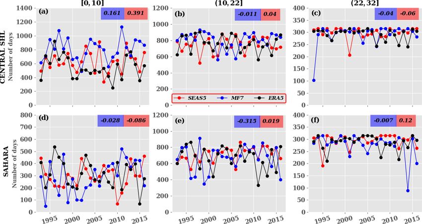
896 C. G. Ngoungue Langue et al.: Seasonal forecasts of the Saharan heat low characteristics
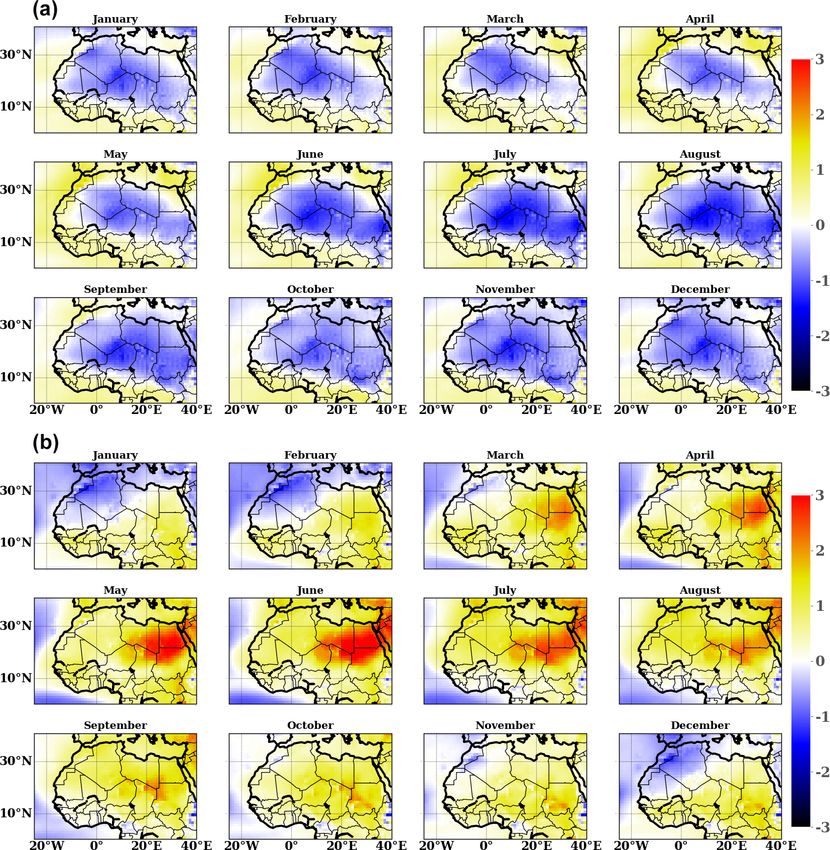
Figure 2. Climatology of the SHL during the JJAS period over 1993–2016 in the reanalysis data using T850, (a) ERA5 and (b) MERRA,
and the anomalies of the climatologies of the SHL between (c) SEAS5 and ERA5, (e) SEAS5 and MERRA, (d) MF7 and ERA5, and (f)
MF7 and MERRA. The rectangles indicate the boxes chosen for the computation of the average T850 and their corresponding name. WSHL:
western SHL; CSHL: central SHL; ESHL: eastern SHL; SAH: the Saharan region. The color bars indicate T850 (a, b) and the anomalies of
T850 (c–f) in kelvins. The computation was made using the ensemble mean member.
period, June–September); Roehrig et al. (2011) show that To be coherent with the model outputs, we consider only
the SHL tends to migrate from the west to the east during the daily temperature data at 00:00 and 12:00 UTC. We also
the season, which explains the WSHL and ESHL locations. transformed the spatial resolution of ERA5/MERRA (from
The Saharan location has been used in some climate studies 0.25◦ ×0.25◦ /0.5◦ ×0.625◦ to 1◦ ×1◦ ) to match the one of the
(Lavaysse, 2015; Taylor et al., 2017). seasonal forecast models. The two forecast models analyzed
here are the seasonal forecast SEAS5 from ECMWF and
2.3 Data the seasonal forecast system MF7 from Météo-France. The
seasonal forecast model SEAS5 replaces the previous sea-
In this study, we used two types of data: reanalyses and sonal system S4 (Johnson et al., 2019); it includes upgraded
seasonal forecast model outputs. We used outputs from versions of the atmosphere and ocean models at higher res-
the fifth-generation European Center for Medium-Range olutions. The SEAS5 model has a horizontal resolution of
Weather Forecasts (ECMWF) Reanalysis (ERA5) (Hersbach 36 km over the globe and contains 91 levels for the vertical
et al., 2020). The ERA5 atmospheric variable studied here is resolution. The MF7 seasonal forecast system is based on
daily T850 with a spatial resolution of 0.25◦ × 0.25◦ down- the ARPEGE/IFS global forecast model (Déqué et al., 1994)
loaded on the climate data store website: https://cds.climate. which was jointly developed by Météo-France and ECMWF.
copernicus.eu/ (last access: 14 January 2020). The Modern- MF7 uses the climate version of CNRM-CM6 (Voldoire
Era Retrospective analysis for Research and Applications et al., 2019) such that MF7 and SEAS5 only share a com-
(MERRA) dataset was also used. The MERRA data have mon radiation parameterization but the rest of the physical
a spatial resolution of 0.5◦ × 0.625◦ with 42 vertical levels package is different. The horizontal resolution of the MF7
downloaded on the ClimServ database. As for ERA5 reanal- model is around 7.5 km over France and 37 km over the An-
ysis, we used the MERRA T850 to carry out our analyses. tipodes; it contains 105 vertical levels. Both SEAS5 and MF7
Weather Clim. Dynam., 2, 893–912, 2021 https://doi.org/10.5194/wcd-2-893-2021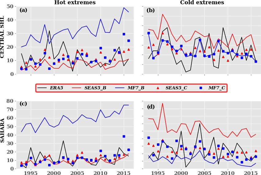
C. G. Ngoungue Langue et al.: Seasonal forecasts of the Saharan heat low characteristics                                      897

model outputs used in this paper are based on the ensemble        by a scale factor and a position factor (Büssow, 2007; Zhao
retrospective forecast (hindcast) which contains 25 members,      et al., 2004).
meaning that for a given time, we have 25 re-forecasts from          Let f (t) be a real function of a real variable; the wavelet
each model. The re-forecasts are released on the first day        transformation of this function denoted as W (f )(a, b) is
of every month for a period of 6 months for SEAS5. With           given by
MF7, one member of the model is initialized on the first of
the month and the other members are launched on the last                                    Z+∞
two Thursdays of the month. The atmospheric variable in-          W (f )(a, b) =< f, ψa,b >= (f (t) · ψa,b (t)dt,             (1)
vestigated in models is also daily temperature at 00:00 and                                        −∞
12:00 UTC with a spatial resolution of 1◦ × 1◦ . Our dataset                  1     t −b
covers the period going from 1 January 1993 to 31 Decem-          ψa,b (t) = √ · 9(      ).                                   (2)
                                                                               a      a
ber 2016.
                                                                     The function 9 is called theR mother wavelet and must be of
                                                                                                   +∞
2.4     Strategy for the analysis of forecast                     square integrable that means −∞ (9(t))2 dt is finite and also
                                                                                                   R +∞
                                                                  verify the following property: −∞ 9(t)dt = 0. The param-
As we analyze the representation of the SHL, we focus on          eter b is the position factor, and a is the scaling parameter
the period going from June to September (denoted by JJAS          greater than zero. For a given signal, a represents the fre-
in the rest of the study) because it corresponds approximately    quency and b the time. There exist diverse types of mother
to the period of maximum heat low activity over the Sa-           wavelets; based on the literature review and its common use,
hara (Lavaysse et al., 2009). Seasonal forecast models usu-       we chose the Morlet wavelet (Tang et al., 2010). The Morlet
ally fail to correctly forecast events a long time in advance     wavelet is defined as the product of a complex sine wave and
for a given target period. Therefore, we are interested in a      a Gaussian window (see Eq. 3) (Cohen, 2018). The wavelet
forecast launched at most 2 months in advance of the JJAS         analysis has been applied separately to the re-forecasts and
period. In order to do that, we consider re-forecasts initial-    the reanalyses for an initialization of the seasonal forecast
ized on 1 April, 1 May and 1 June, which corresponds to a         models on 1 April, 1 May and 1 June for a 6-month period;
June lead time of 2, 1 and 0 months respectively. This tech-      but we extracted only the signal on the JJAS period to con-
nique allows us to quantify the sensitivity of the models in      duct our analyses on variability modes. We focused on sig-
representing the SHL at different lead times. The re-forecast     nals with a period of up to 32 d.
validation process is made separately for the whole JJAS pe-
riod and individual months (June, July, August and Septem-                              2 /2
ber) because June and September temperature values are in         9(t) = π −1/4 exp−t          cos(wo t)                      (3)
the same range.
                                                                  2.5.2   Bias correction
2.5     Methods                                                   Seasonal forecast models provide a numerical representation
                                                                  of the Earth and the interactions between its different compo-
This section describes in more detail the set of analyses car-    nents: the atmosphere, the ocean and the continental surfaces.
ried out to achieve our goal. The methodology adopted is          Those interactions are very complex and take place at differ-
illustrated below.                                                ent spatio-temporal scales. This can lead in certain cases to
                                                                  an over/underestimation of the evolution of atmospheric vari-
2.5.1    Subseasonal modes of variability                         ables in the models. The cause of this behavior in the models
                                                                  is often the presence of biases. To overcome this bias issue,
A mode of variability represents a spatio-temporal structure      we use here two univariate bias correction methods: quan-
highlighting the main characteristics of the evolution of at-     tile mapping (QMAP) and cumulative distribution function
mospheric variables at a given timescale. There are several       transform (CDF-t).
statistical methods for assessing the modes of variability that
contribute to a raw signal. The one used here is the wavelet      QMAP
analysis of the temperature signal. The wavelet transform
consists in applying a time–frequency analysis to a given sig-    Quantile mapping aims to adjust climate model simulations
nal. It is very useful for analyzing non-stationary signals in    with respect to reference data, in determining a transfer func-
which phenomena occur at different scales. This method pro-       tion to match the statistical distribution of simulated data to
vides more information than the Fourier transform about the       one of the reference values (e.g., Dosio and Paruolo, 2011).
observed structures in the initial signal (starting and ending    When reference data have a resolution similar to those of cli-
time and the duration of propagation (frequency)). With this      mate model simulations, this technique can be considered a
type of analysis, we observe the distribution of the signal in-   bias adjustment method. On the other hand, when the obser-
tensity in time and frequency. A wavelet function is defined      vations are of a higher spatial resolution than those of climate

https://doi.org/10.5194/wcd-2-893-2021                                              Weather Clim. Dynam., 2, 893–912, 2021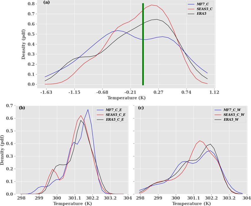
898                                    C. G. Ngoungue Langue et al.: Seasonal forecasts of the Saharan heat low characteristics

simulations, quantile mapping attempts to fill the scale shift        to the raw re-forecasts will be assessed by the computation
and is then considered a downscaling method (Michelangeli             of the Cramér–von Mises (hereafter Cramér) score (Henze
et al., 2009). The QMAP method is based on the assump-                and Meintanis, 2005; Michelangeli et al., 2009). The Cramér
tion that the transfer function calibrated over the past period       score measures the similarity between two distribution func-
remains valid in the future. Let Fo, h and Fm, h be the cumu-         tions; the closer its value is to 0, the closer the distributions
lative distribution functions (CDFs) of the observational (ref-       are.
erence) data Xo, h and modeled data Xm, h respectively, in a
historical period h. The transfer function for bias correction
                                                                      Application of bias correction
of Xm, p (t) which represents a modeled value at time t within
a projected period p is given by the following relation (e.g.,
Cannon et al., 2015; Dosio and Paruolo, 2011):                        QMAP and CDF-t are usually used for downscaling tasks in
                                                                      a climate projection context. In this study, we adapted the
                                                                      application of these methods for bias correction in a seasonal
X̂m, p (t) = Fo,−1h {Fm, h [Xm, p (t)]},                       (4)    forecast context. We used a leave-one-out approach for the
                                                                      calibration process with CDF-t and QMAP. This method con-
where Fo,−1h is the inverse function of the CDF Fo, h .               sists in removing the target year (the year we want to apply
                                                                      the correction to) in the historical period before the estima-
CDF-t                                                                 tion of the transfer function which allows us to pass from
                                                                      the global scale to local-scale data. In our case the calibra-
CDF-t is a statistical downscaling method developed by                tion process has been made using 23 of the 24 years in the
Michelangeli et al. (2009). It can be considered a general-           historical period 1993–2016 for every year. The correction
ization of the quantile-mapping correction method. Hence,             or projection process is made differently using CDF-t and
as with QMAP, CDF-t consists in finding a relationship be-            QMAP. For QMAP, we use as input the target year removed
tween the CDF of a large-scale climate variable and the CDF           previously during the calibration phase. With CDF-t, we built
of this same variable at the local scale. However, while the          a new dataset of 24 years which is the concatenation of the
quantile-mapping method projects the simulated values at a            dataset used for the calibration and the target year so that the
large scale on the historical CDF to calculate quantiles, CDF-        year at the end of the new dataset represents the target year.
t takes explicitly into account the change in the large-scale
CDF between the historical period and the future period. In
the CDF-t approach, a mathematical transformation T is ap-            2.5.3   Ensemble forecast verification
plied to the large-scale CDF to define a new CDF as close
as possible to the CDF obtained from the station data (e.g.,          Ensemble forecast verification is the process of assessing the
Vrac et al., 2012; Lavaysse et al., 2012).                            quality of a forecast. The forecast is compared against a cor-
   Let Fm, h and Fo, h be the CDFs at a large and local scale         responding observation or a reference; the verification can
respectively of the modeled data Xm, h and the observational          be qualitative or quantitative. Forecast verification is impor-
data Xo, h over a historical period h and T the transformation        tant for monitoring forecast quality, improving forecast qual-
allowing us to go from Fm, h to Fo, h . We have the following         ity and comparing the quality of different forecast systems.
relation (Vrac et al., 2012):                                         There are many metrics or probability scores developed for
                                                                      ensemble forecast verification depending on the tasks per-
                                                                      formed. In our preliminary studies (not shown) on the skills
T (Fm, h (Xm, h )) = Fo, h (Xo, h ).                           (5)
                                                                      of the forecast models, we used different scores (continuous
   By applying this relation to the CDF Fm, f of the modeled          ranked probability score – CRPS, Brier score, relative oper-
data Xm, f in a future period f, it provides an estimation of the     ating characteristic (ROC) area curve, rank histogram, relia-
local CDF Fo, f in the future period f:                               bility diagram), but in the present work, we will only focus
                                                                      on the CRPS (Hudson and Ebert, 2017), which is very simi-
                                                                      lar to the Brier score. This choice is justified by the simplicity
F̂o, f = T (Fm, f (Xm, f )).                                   (6)    in data processing when computing the CRPS through some
                                                                      R packages like SpecsVerification (Siegert et al., 2017). The
   Quantile mapping can then be performed between Fm, f               CRPS is a quadratic measure of the difference between the
and F̂o, f to obtain bias-corrected values of future simula-          forecast CDF and observation CDF. It quantifies the relative
tions. More details about CDF-t can be found in Vrac et al.           error between the model forecasts and the observations; it is
(2012). All the computations for the CDF-t method were                a measure of the precision of an ensemble forecast model.
done with the R package “CDFt”.                                       The closer the CRPS is to 0, the better it is.
   After applying the bias correction methods to the model               Letting PF (x) and PO (x) be the cumulative distribution
outputs, the added value of the bias correction compared              functions for the forecasts and observations respectively, the

Weather Clim. Dynam., 2, 893–912, 2021                                                    https://doi.org/10.5194/wcd-2-893-2021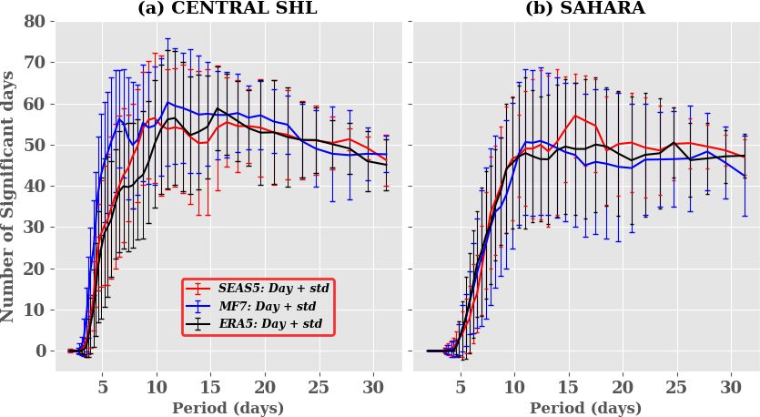
C. G. Ngoungue Langue et al.: Seasonal forecasts of the Saharan heat low characteristics                                      899

CRPS is computed as follows:                                      3.2   Variability modes

       Z+∞                                                        Through a wavelet transformation, we compared the vari-
CRPS =    (PF (x) − PO (x))2 dx                            (7)    ability modes in the forecast products (SEAS5, MF7) with
          −∞                                                      respect to ERA5 over the central SHL location and Sahara
                                                                  (boxes indicated in Fig. 2) (see Fig. S4 in the Supplement).
   The root mean square error (RMSE), which is a measure          Especially for the year 2016, three main frequency bands of
of the differences between two samples (model predictions         activity of the SHL have been identified in ERA5: firstly,
and observations), has also been used for the evaluation of       the SHL activity within the 4–8 d window with high inten-
the forecasts. Letting yt be the forecast of the model at time    sity; secondly an intensification of events with strong inten-
t and Ot the corresponding observation at the same time, the      sity (spectral power > 16) is observed for periods of about
RMSE is given by the following relation:                          8–16 d. Finally, events at very high frequencies are observed,
                                                                  and the intensity associated is much higher (spectral power >
           s
                PN                                                64) than in the previous ones. This shows the SHL activity
                 t=1 (yt   − Ot )2                                becomes stronger at high frequencies. The models tend to
RMSE =                               ,                     (8)
                      N                                           reproduce the pulsations observed in the reanalysis signals
                                                                  quite differently; there is an issue regarding the temporality,
where N is the number of time steps.                              frequency and intensity of the pulsations in the forecast mod-
                                                                  els.
3     Results                                                        To assess the climatology of the variability modes (Fig. 3),
                                                                  we analyzed the distribution of days associated with spectral
3.1    Climatology of the SHL                                     power greater than 1 (normalized value), here defined as sig-
                                                                  nificant days during the period 1993 to 2016. This threshold
The climatology state of the SHL has been assessed from           of 1 has been selected arbitrarily after applying a sensitivity
1993 to 2016 during the JJAS period for ERA5, MERRA,              test to several threshold values from 0.5 to 10 to focus on
SEAS5 and MF7 (see Fig. S2 in the Supplement). The sea-           predominant events at different periods. We noticed globally
sonal forecast models tend to develop SHL’s climatologies         a decrease in events occurrence with high threshold values of
with very similar characteristics to those of the reanalyses.     the spectral power. Note that the sensitivity to the threshold
Strong SHL intensities are located over the CSHL location         values does not significantly impact our results (not shown).
(Fig. S2) for all the products (reanalyses and forecast mod-      We observe similar behavior in ERA5, SEAS5 and MF7 in
els); this is in agreement with Lavaysse et al. (2009). Another   terms of significant days with an increasing number of days
point discussed in this section is the uncertainty between        with periods of up to 10 d followed by quite steady activity
the reanalyses (ERA5 and MERRA) (see Fig. 2). ERA5 and            for longer periods. Over the Sahara area, there is a tendency
MERRA exhibit similar behaviors regarding the climatologi-        for both models to reproduce SHL activity that is similar to
cal bias of the SHL with respect to the seasonal forecast mod-    ERA5 at too-short periods (∼ 10 d). ERA5 shows little vari-
els (Fig. 2c–f): a cold bias with SEAS5 and a warm bias with      ation in the number of significant days with periods between
MF7. The seasonal evolution of the climatological state of        12–26 d and tends to be constant for high-frequency peri-
the SHL in ERA5 and MERRA (see Fig. 6) is almost similar          ods (greater than 27 d). SEAS5 overestimates the SHL ac-
over the CSHL location except for the Sahara, where a little      tivity around the 15 d period, while MF7 is shifted toward
shift of MERRA to high temperatures is observed but the pat-      higher frequencies and underestimates the longer period.
terns in the evolution remain very close to ERA5. The distri-     Over the central SHL box, there is a tendency of both the
bution of yearly T850 over the JJAS period (see Fig. 7a, b, g,    MF7 and the SEAS5 models to generate significant SHL ac-
h) in ERA5 and MERRA is quite similar, suggesting a good          tivity at too-short periods (∼ 4/10 d) compared to ERA5. At
correlation between the two reanalyses. The uncertainties be-     longer timescales MF7 tends to overestimate the SHL activ-
tween the reanalyses (see Fig. S3 in the Supplement) are          ity within the 10–23 d period, while SEAS5 shows an under-
much smaller than the biases in the seasonal forecast mod-        estimation of the SHL activity within the same window. The
els with respect to ERA5. We also found large correlation         evolution of significant days over the central SHL location
between ERA5 and MERRA (see Fig. S1 in the Supplement)            and Sahara highlighted three main pulsations based on the
of around 0.97/0.92 over the CSHL/Sahara location during          period (or frequency). The different pulsations identified are
the JJAS period. By considering all these results highlighting    arbitrarily classified as follows: the class C1 = [0, 10] d for
high similarities between ERA5 and MERRA, we decided              low-frequency, the class C2 = (10, 22] d for high-frequency
to choose ERA5 as our reference dataset for the rest of the       and the class C3 = (22, 32] d for very high frequency pulsa-
study.                                                            tions. In the following, we investigate the interannual vari-
                                                                  ability of significant days for those different classes of pulsa-
                                                                  tion (Fig. 4). The result for ERA5 shows a high interannual

https://doi.org/10.5194/wcd-2-893-2021                                              Weather Clim. Dynam., 2, 893–912, 2021
900 C. G. Ngoungue Langue et al.: Seasonal forecasts of the Saharan heat low characteristics
variability for pulsations in class C1 over both the central less affected by this warming in MF7 compared to the rest of
SHL box and the Sahara (Fig. 4a, d). This can be caused by the Sahara. This behavior in the Sahara region, especially in
the triggering of easterly waves and Kelvin equatorial waves the eastern part of the Sahara, could be related to an under-
which tend to reinforce the convection activity. Those two estimation of air advection coming from the Mediterranean
types of wave have a periodicity of between 1–6 d (Janicot regarding the prevalence of the hot bias to the eastern part of
et al., 2008a). The correlation between the seasonal forecast the Sahara (Fig. 2b). This analysis shows that the two sea-
models and ERA5 is very low, less than 0.4. From this anal- sonal forecast models have two contrasted representations of
ysis, we can see that the seasonal forecast models tend to the SHL compared to ERA5, with a colder SHL in SEAS5
represent the climatological activity of the SHL at different and a warmer SHL in MF7, which is in agreement with pre-
frequencies even if some discrepancies are observed. How- vious global studies (e.g., Dixon et al., 2017; Johnson et al.,
ever, the representation of the interannual variability in the 2019). The two seasonal forecast models share however a
SHL activity remains a big challenge for the seasonal fore- similar seasonal evolution of the bias (increasing bias during
cast models. the monsoon season) and a large spatial scale of the bias that
covers most of the Sahara. Without sensitivity experiments,
3.3 Seasonal cycle it is impossible to clearly identify the reasons for these op-
posite behaviors between the two models. The investigation
In this section, we are assessing the spatial representation of of the origins of these biases is well beyond the scope of
the SHL over the Sahara region. In order to do that, we eval- this article. In a more general framework, various European
uate the bias between the seasonal forecast models (SEAS5, research projects have shown the difficulty of attributing a
MF7) and ERA5 (Fig. 5). The bias is defined here as the dif- specific bias to a specific parameterization over West Africa,
ference between the forecasts and the reanalyses; the mathe- including the SHL (Martin et al., 2017).
matical expression of the bias is the following: After the evaluation of the spatial evolution of the SHL in
the seasonal forecast models, the representation of the tem-
Bt = Ft − Rt , (9) poral drift is assessed (Fig. 6). The method used here con-
sists in computing the climatology of the daily T850 ensem-
where Ft and Rt are the forecasts and reanalyses respectively ble mean and ensemble spread for the two models (SEAS5
at time t. and MF7) and the daily climatology of T850 for ERA5
The bias is computed for each month at lead time 0 during from 1993–2016. For the models, we consider only the re-
the season from January to December for the period 1993– forecasts launched on 1 April, 1 May and 1 June for a pe-
2016. By extending the analysis window over the season, we riod of 6 months (see Sect. 2.4 for more details). We can
are able to check if the biases in the seasonal forecast mod- see that the climatology of ERA5 remains contained in the
els are constant or specific to the JJAS period. When an- spread described by SEAS5 for all lead times over the cen-
alyzing the SEAS5 model outputs (Fig. 5a), we notice an tral SHL location and Sahara; this spread in SEAS5 seems
overestimation of temperature over the Atlantic Ocean and to be constant in time and does not increase with the lead
over the Mediterranean Sea. We observe a cold bias between time. We observe for the first forecast days a large spread
SEAS5 and ERA5 which appears progressively during the with MF7 which is not present in SEAS5, likely associated
first months (January to April) and tends to intensify during with different perturbations and initialization techniques that
the monsoon phase over the Sahel region. This cold bias is are beyond the scope of this study. For all lead times, an
centered over the Sahara between the north of Mali, Niger overestimation of temperature is shown with MF7 over the
and the south of Algeria and tends to decrease in intensity Sahara around mid-June and later over the central SHL loca-
during the retreat phase of the monsoon in October. SEAS5 is tion (∼ 10 d after 1 July). SEAS5 shows an underestimation
colder than ERA5 and underestimates the spatial evolution of of temperature occurring on 1 July over both the central SHL
the SHL over the Sahara. In fact, biases in the evolution of the box and the Sahara at different lead times. The maximum
coupled ocean–atmosphere system or in the continental sub- intensities of the SHL activity in the two seasonal forecast
surface can play a role in theses biases, but their investigation models are reached during the period of strong activity of the
is beyond the scope of this paper. The analysis on MF7 shows monsoon flux in the Sahel region (July–August). Both mod-
a progressive appearance of a warm bias in comparison to els are very consistent at the beginning of the season (April–
ERA5 over the Sahel during January and February (Fig. 5b). June) when the Sahara is gradually warming. In the extension
This warm bias tends to develop from March to September of the previous analyses, we decided to check the temporal
and affects the whole Sahara. It is more intense during the correlation of the models and ERA5 (Fig. S6). We observe
monsoon phase and is located over the eastern part of the Sa- a weak correlation between the evolution of the SHL in the
hara. The bias between MF7 and ERA5 tends to decrease in seasonal forecast models and ERA5. The scatterplot analysis
intensity during the retreat phase of the monsoon in October. used for this evaluation highlights the over/underestimation
MF7 is warmer than ERA5 and overestimates the spatial evo- of T850 in MF7/SEAS5 with respect to ERA5 as observed in
lution of the SHL over the Sahara. The central SHL area is the monthly bias analyses (Fig. S6c).
Weather Clim. Dynam., 2, 893–912, 2021 https://doi.org/10.5194/wcd-2-893-2021C. G. Ngoungue Langue et al.: Seasonal forecasts of the Saharan heat low characteristics 901 Figure 3. Climatology of significant days: significant days here refer to days with a spectral power signal greater than 1. Red, blue and black curves and bars represent the number of days and spread for SEAS5, MF7 and ERA5 respectively over the (a) central SHL box and (b) Sahara during the period 1993–2016. The computation was made just using the unperturbed member of the ensemble forecast models launched from 1 June for the JJAS period. The y axis represents significant days and x axis the duration of propagation in days. Figure 4. Interannual variability of significant days: significant days here refer to days with a spectral power signal greater than 1. Red, blue and black curves represent the number of days for SEAS5, MF7, ERA5 respectively over the (a–c) central SHL and (d–f) Sahara. The values in red and blue boxes refer to the correlation between SEAS5 and ERA5 and between MF7 and ERA5 respectively. The terms [0, 10], (10, 22] and (22, 32] are the different classes of days identified for the present study. The computation was made just using the unperturbed member of the ensemble forecast models launched from 1 June for the JJAS period. The y axis represents significant days and x axis the year. An estimation of bias was carried out for the SEAS5 model smaller cold bias compared to in SEAS52 . This change in data for (i) the full available period, running from 1981 to bias intensity can be explained by a warming in SEAS5 re- 2016 (denoted SEAS51 ), and (ii) the period common to MF7 forecasts during the period 1981–1992 which attenuates the and SEAS5, 1993–2016 (denoted SEAS52 ). The bias evolu- cooling effect in the model during the period 1993–2016. tion is quite similar over the two periods (see Fig. 5a and Fig. S5 in the Supplement); but we notice in SEAS51 a https://doi.org/10.5194/wcd-2-893-2021 Weather Clim. Dynam., 2, 893–912, 2021
902                                C. G. Ngoungue Langue et al.: Seasonal forecasts of the Saharan heat low characteristics

Figure 5. Climatology of monthly bias temperature over the Sahara region during 1993–2016 between (a) SEAS5 and ERA5 and (b) MF7
and ERA5. The bias is computed using daily temperature at 00:00 and 12:00 UTC. The computation was made using the ensemble mean for
forecast models. The color bar indicates the bias value in kelvins. The y axis indicates the latitudes and x axis the longitudes of our domain.

3.4   Interannual distribution of the T850                                SEAS5 tends to represent much better than MF7 the distribu-
                                                                          tion the SHL intensities over the Sahara (Fig. 7a, c, d and g, i,
The climatological trend of the distribution of SHL intensi-              j). Another specificity of MF7 is its slightly larger ensemble
ties has been analyzed using the seasonal probability distri-             spread. SEAS5 seems to underestimate the warming trends
bution function (pdf) (Fig. 7a, f) of the SHL box-averaged                present in ERA5 from 2005–2016, and an overestimation of
T850 (used as the proxy for the SHL intensity) over the JJAS              this trend is observed with MF7 (Fig. S10); this behavior in
period at June lead time 0 (i.e., the initialization of the model         the seasonal forecast models is present over both the central
was made on 1 June). The analysis of seasonal T850 shows a                SHL box and the Sahara. By using this type of visualization
high variability in ERA5 and the presence of a decadal warm-              (heatmap which is a graphical representation of data where
ing trend from 2005–2016 over both the central SHL location               values are depicted by color), it is possible to assess the inten-
and the Sahara (Fig. 7a, g). The high interannual variabil-               sity of the climatological trend with respect to the intrasea-
ity in the SHL seen in ERA5 is underestimated by SEAS5                    sonal variability (Fig. 8). The interannual variability in the
and MF7. Using raw outputs of the seasonal forecast models,

Weather Clim. Dynam., 2, 893–912, 2021                                                         https://doi.org/10.5194/wcd-2-893-2021
C. G. Ngoungue Langue et al.: Seasonal forecasts of the Saharan heat low characteristics 903
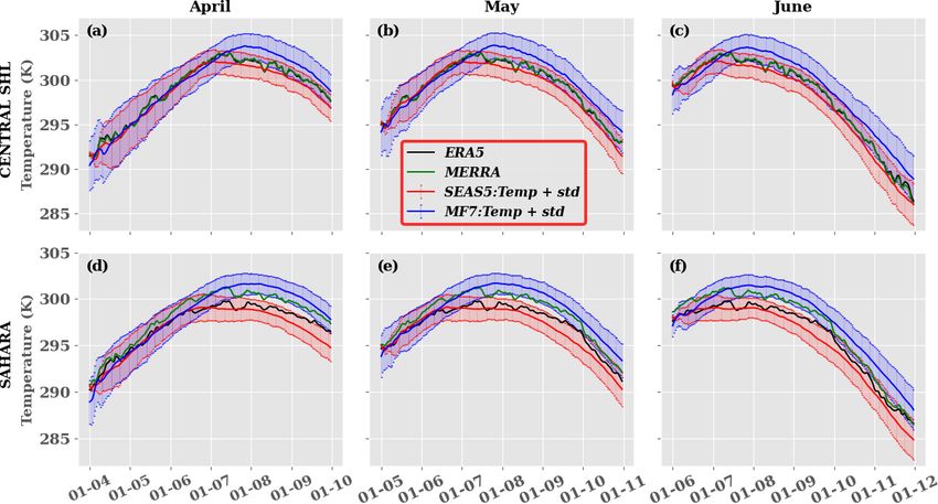
Figure 6. Climatology and spread of mean daily temperature during 1993–2016 at different initialization months for a 6-month forecast:
(a, d) April, (b, e) May and (c, f) June for the (a–c) central SHL box and (d–f) Sahara. Bold black, green, red and blue curves refer to the
mean T850 of ERA5, MERRA, SEAS5 and MF7 respectively; red and blue bars represent the inter-member spreads for SEAS5 and MF7
respectively. The computation was made using the ensemble mean of forecast models. The y axis indicates temperature in kelvins and x axis
the time.
SHL anomalies distribution in the seasonal forecast models is because of the many possible ways to approach the bias cor-
too far from ERA5, but some characteristics are captured by rection; i.e., should we use the unperturbed member, mean
the models (e.g., the increase in the frequency of anomalies ensemble member, median ensemble member or the whole
in ERA5 during the 2000s). We observed high frequencies in ensemble member? In our case, the bias correction is first ap-
the SHL anomalies distribution at an interannual timescale plied separately to the ensemble members in order to correct
for MF7 and SEAS5 with more intense values over the Sa- the re-forecasts of each of the 25 members of the seasonal
hara (Fig. 8b, c, g, h). To focus more on the evolution of the forecast models (SEAS5 and MF7). A second methodology
tails of the distribution (i.e., the warmest and coldest T850), has been tested by applying a bias correction to the ensem-
the anomaly of the pdf of temperature is provided in supple- ble mean. To evaluate the sensitivity of the Cramér score to
mentary materials (Fig. S7). An increase in the occurrence the ensemble forecast models, we defined three different ap-
of the warmest temperature is observed in SEAS5 and MF7 proaches as follows:
during the 2010s. MF7 tends to overestimate the interannual
variability in the coldest and warmest temperature distribu- – CORR_NO_MEAN. In this approach the bias correc-
tion, and SEAS5 exhibits an overall trend with some features tion is applied to the whole ensemble member and the
close to ERA5. Despite the fact that seasonal models tend Cramér score is computed using the outputs of the cor-
to capture some characteristics of the SHL variability, large rection.
differences are observed in comparison with ERA5. These – CORR_MEAN. Here we compute first the mean over the
differences can be explained by systematic biases present in outputs of the bias correction on the whole ensemble
models, as well as by approximations made during the mod- member; and we use this mean to compute the Cramér
els implementation (initial and boundary conditions, physi- score;
cal hypotheses, etc.). In order to improve the quality of the
forecast, bias correction methods have been applied. – MEAN_CORR. The method consists of applying the
The above analyses revealed the presence of biases in the bias correction to the ensemble mean, and the computa-
models; bias correction was applied over the JJAS period for tion of the Cramér is performed directly using the out-
June lead times 2, 1 and 0 (which represent the forecast of the puts of the correction.
JJAS period initialized in April, May and June respectively).
The bias correction techniques used are CDF-t and QMAP The Cramér score was calculated firstly using ERA5 and
(see Sect. 2.5.2 for more details on their application). The the raw forecast samples (SEAS5 and MF7) and secondly be-
analysis of ensemble forecast models remains very delicate tween ERA5 and the bias-corrected forecast samples (Fig. 9).
We can observe that raw forecasts are not improved with
https://doi.org/10.5194/wcd-2-893-2021 Weather Clim. Dynam., 2, 893–912, 2021904 C. G. Ngoungue Langue et al.: Seasonal forecasts of the Saharan heat low characteristics Figure 7. Distribution of yearly T850 over the JJAS period during 1993-2016 over the (a–f) central SHL box and (g–l) Sahara. ERA5, MERRA, SEAS5_BRUT and MF7_BRUT here correspond to the intensity of the SHL using ERA5 and MERRA for the reanalyses; SEAS5 and MF7 raw forecasts respectively. SEAS5_CDFT and MF7_CDFT refer to the intensity of the SHL using SEAS5 and MF7 seasonal forecasts respectively bias corrected using ERA5. The computation was made using the ensemble members of the forecast models. The y axis indicates time in years and x axis T850 in kelvins. The color bar indicates the probability of occurrence. Figure 8. Same as Fig. 7 but for the yearly anomalies of temperature. The anomalies are computed by removing the daily climatology temperature for each year. initialization months (April, May or June) while corrected model outputs. Some illustrations of the corrected forecasts forecasts show an improvement with decreasing lead times. have been made with the CDF-t method. In Fig. 7e and j, we This can be the result of systematic bias in seasonal forecast can notice a significant improvement in the distribution of models. The MEAN_CORR method (Fig. 9c, f, i) is more SHL in MF7 over both the central SHL location and the Sa- efficient than the two other approaches CORR_MEAN and hara. This improvement is also effective for SEAS5 (Fig. 7d, CORR_NO_MEAN, based on the Cramér score values. The i). The corrected forecast distributions are closer to ERA5 CORR_MEAN approach tends to smooth the corrected fore- than the raw forecast ones. The investigation of the correla- casts due to the computation of the mean ensemble mem- tion between the corrected forecasts and ERA5 (Fig. S6b, ber after applying the correction. CDF-t and QMAP meth- d) shows clearly that CDF-t corrects the cold/hot bias in ods produce very similar results; an illustration of the cor- SEAS5/MF7 by increasing/decreasing T850 values in order rected forecasts using both the methods is provided in sup- to match with ERA5 T850 values. CDF-t reduces a large plementary materials (see Fig. S9). MF7 raw forecasts show part of the biases in SEAS5 and MF7, but the interannual relatively large correction over the Sahara (Fig. S8); this be- correlation with ERA5 is not improved. Indeed, CDF-t is a havior in MF7 is related to the hot bias occurring over the quantile-based univariate bias adjustment method. As such, eastern part of Sahara during the JJAS period as mentioned it preserves the ranks of the model simulations and thus pre- in Sect. 3.2 (Fig. 5b). We can see from these results that serves their rank (Spearman) correlations as well (e.g., Vrac, bias corrections are efficient and so important to apply to the 2018; François et al., 2020). Weather Clim. Dynam., 2, 893–912, 2021 https://doi.org/10.5194/wcd-2-893-2021
C. G. Ngoungue Langue et al.: Seasonal forecasts of the Saharan heat low characteristics                                      905

Figure 9. Bias correction evaluation using Cramér–von Mises score over the JJAS period during 1993–2016 on the central SHL box at
different forecast initialization months: (a–c) April, (d–f) May and (g–i) June. The CORR_NO_MEAN, CORR_MEAN and MEAN_CORR
methods are well described in Sect. 3.4. S5_B, S5_CD and S5_QM represent the Cramér score computed using the SEAS5 raw forecasts,
SEAS5 corrected with CDF-t and QMAP methods respectively. The same applies to MF7_B, MF7_CD and MF7_QM with the MF7 model.
The y axis indicates the Cramér score and x axis the different products used for the computation of the Cramér score.

3.5   Evolution of the extreme SHL events                          difference between ERA5 and the corrected forecasts being
                                                                   reduced compared to the raw forecasts, the observed gap re-
                                                                   mains significant.
Strong SHL activity contributes to the reinforcement of the
monsoon flow over the Sahel along the eastern flank of the         3.6   East–west pulsation modes
SHL. It also modulates the intensity of the AEJ and gener-
ates wind shear over the region. The resulting wind shear          The SHL has a typical timescale of 15 d associated with low-
will generate more instabilities favoring convective activi-       level horizontal advection of moist and cold air that modu-
ties over the West Africa region. Taylor et al. (2017) showed      lates the surface temperature on the eastern part of the Sa-
that strong SHL activity intensifies the convection within         hara and makes the maximum surface temperature shift from
the meso-scale convective systems (MCSs). Fitzpatrick et al.       a more eastern to a more western location of the Sahara
(2020) suggest that stronger wind shear may be a key driver        (Chou et al., 2001; Roehrig et al., 2011), leading to so-called
of decadal changes in storm intensity in the Sahel. This           heat low east (HLE) events and heat low west (HLW) events
shows the importance of having a good representation of            respectively (Chauvin et al., 2010). Roehrig et al. (2011)
these SHL characteristics in the models. Therefore, we an-         and Lavaysse et al. (2011) highlighted interactions between
alyzed the variability in the SHL extremes using the raw and       SHL components and Sahelian rainfall events. In the present
corrected forecasts obtained with CDF-t (Fig. 10). We distin-      work, a simple method is proposed to capture the HLW and
guished cold and hot extremes which represent events under         HLE oscillations. Our method consists in defining a dipole
the quantile 10 % and above the quantile 90 % respectively.        by computing the mean T850 difference between HLW and
We observe an increase in the SHL hot extremes in the sea-         HLE boxes, here referred to as WSHL and ESHL respec-
sonal forecast models during the 2010s as well as a diminu-        tively (see Sect. 2.2 for more details):
tion of the SHL cold extremes which is in agreement with
the evolution in ERA5. MF7 raw forecasts tend to overesti-
                                                                   Dipole = H LW − H LE                                      (10)
mate the SHL hot extremes, while they seem to underesti-
mate the SHL cold extremes over both the central SHL loca-            A positive value of the dipole indicates an HLW oc-
tion and the Sahara. SEAS5 raw forecasts underestimate the         currence, while a negative value corresponds to the HLE
SHL hot extremes and make an overestimation of the SHL             event. We evaluate the method using the LLAT approach
cold extremes over the Sahara. We can see the efficiency of        and the automatic detection of the SHL barycenter (Lavaysse
the bias correction (CDF-t) when analyzing the evolution of        et al., 2009) used during the H2020 Dynamics–Aerosol–
the SHL extremes from the corrected forecasts. Despite the         Chemistry–Cloud Interactions in West Africa (DACCIWA)

https://doi.org/10.5194/wcd-2-893-2021                                              Weather Clim. Dynam., 2, 893–912, 2021
906 C. G. Ngoungue Langue et al.: Seasonal forecasts of the Saharan heat low characteristics
Figure 10. Interannual variability in the SHL extremes over the (a, b) central SHL and (c, d) Sahara during the JJAS period from 1993 to
2016. SEAS5_C and MF7_C refer to corrected forecasts with the CDF-t method, and SEAS5_B and MF7_B represent raw model forecasts.
The x axis indicates the time (year) and y axis the number of extremes registered for each year. Hot extremes are events occurring above the
90th percentile, and cold extremes are associated with events below the 10th percentile.
project campaign (Knippertz et al., 2017), which aims to Table 1. Correlation between the dipole values derived from the
evaluate the seasonal location of the SHL with respect to seasonal models (SEAS5 and MF7) and the one derived from
its climatological position. An illustration of our method for ERA5. The “Raw dipole” represents the dipole computed using raw
the year 2005 is shown in Fig. S11 and confirms that there forecasts and “Corrected dipole” that using the bias-corrected fore-
is a good agreement between the evolution of the dipole of casts.
T850 in ERA5 and the SHL barycenter computed in Knip-
SEAS5 MF7
pertz et al. (2017). After the assessment of the detection
method, we evaluate the representation of the SHL compo- Raw dipole 0.53 0.65
nents in the seasonal forecasts and ERA5 data (Fig. 11a). Corrected dipole 0.61 0.75
As the corrected forecasts are unbiased compared to the raw
forecasts, we use them for this analysis. The results show that
ERA5 presents a bimodal regime; the first one is less accen- SHL components. The analysis of the correlation between
tuated and associated with the HLE events (negative dipole the models and ERA5 shows that MF7 seems to be slightly
value), while the second regime is more representative and better correlated with ERA5 than SEAS5 (see Table 1). We
related to HLW events (positive dipole value). For MF7, we noticed a little and not significant improvement in the corre-
also noticed a bimodal regime and a large range in the dis- lation with the corrected signal.
tribution of the dipole compared to ERA5; the first regime To better understand the reasons for these differences, a
is more frequent and associated with the HLE events. The separate analysis of the SHL distribution in the two boxes
second regime is less frequent and related to HLW events. is performed (Fig. 11b, c). First, it is worth noting that the
With SEAS5, we also observed a bimodal regime and a re- east Sahara is climatologically hotter than the west Sahara in
duced range compared to ERA5. The first regime is less im- ERA5, SEAS5 and MF7. This is explained by the proximity
portant and associated with the HLE events, while the second of the west Sahara to the Atlantic Ocean and the advection
one is more important and related to HLW events. From this of fresh air masses in that area (see Fig. 2 for the location
analysis, we can notice that MF7 (SEAS5) tends to overes- of the west Sahara). Hence, there is a greater occurrence of
timate the HLE (HLW) phases (Fig. 11a). This behavior in the HLE events compared to the HLW phases in ERA5. The
the seasonal models is well highlighted when using the raw models (SEAS5/MF7) are able to reproduce this partitioning
forecasts for the computation of the dipole (see Fig. S16a in of the SHL phases observed in ERA5 with the same range
the Supplement). MF7 and SEAS5 here again exhibit oppo- of frequencies (∼ 0.6/0.4) for HLE/HLW respectively. Both
site behaviors in terms of frequencies and intensities of the models overestimate the occurrence of the HLE events; MF7
Weather Clim. Dynam., 2, 893–912, 2021 https://doi.org/10.5194/wcd-2-893-2021You can also read