THE MOSAIC ICE FLOE: SEDIMENT-LADEN SURVIVOR FROM THE SIBERIAN SHELF
←
→
Page content transcription
If your browser does not render page correctly, please read the page content below
The Cryosphere, 14, 2173–2187, 2020
https://doi.org/10.5194/tc-14-2173-2020
© Author(s) 2020. This work is distributed under
the Creative Commons Attribution 4.0 License.

The MOSAiC ice floe: sediment-laden survivor
from the Siberian shelf
Thomas Krumpen1 , Florent Birrien1 , Frank Kauker1 , Thomas Rackow1 , Luisa von Albedyll1 ,
Michael Angelopoulos1 , H. Jakob Belter1 , Vladimir Bessonov2 , Ellen Damm1 , Klaus Dethloff1 , Jari Haapala3 ,
Christian Haas1 , Carolynn Harris4 , Stefan Hendricks1 , Jens Hoelemann1 , Mario Hoppmann1 , Lars Kaleschke1 ,
Michael Karcher1 , Nikolai Kolabutin2 , Ruibo Lei5 , Josefine Lenz1,6 , Anne Morgenstern1 , Marcel Nicolaus1 ,
Uwe Nixdorf1 , Tomash Petrovsky2 , Benjamin Rabe1 , Lasse Rabenstein7 , Markus Rex1 , Robert Ricker1 , Jan Rohde1 ,
Egor Shimanchuk2 , Suman Singha8 , Vasily Smolyanitsky2 , Vladimir Sokolov2 , Tim Stanton9 , Anna Timofeeva2 ,
Michel Tsamados10 , and Daniel Watkins11
1 Alfred Wegener Institute, Helmholtz Centre for Polar and Marine Research, Am Handelshafen 12,
27570 Bremerhaven, Germany
2 Arctic and Antarctic Research Institute, Ulitsa Beringa, 38, Saint Petersburg, 199397, Russia
3 Finnish Meteorological Institute, Marine Research, P.O. Box 503, 00101 Helsinki, Finland
4 Dartmouth College, Department of Earth Science, 6105 Fairchild Hall, Hanover, NH 03755, USA
5 Polar Research Institute of China, MNR Key Laboratory for Polar Science, 451 Jinqiao Road,

Pudong, Shanghai 200136, China
6 Association of Polar Early Career Scientists, Alfred Wegener Institute for Polar and Marine Research,

Telegrafenberg A45, 14473 Potsdam, Germany
7 Drift & Noise Polar Services, Stavendamm 17, 28195 Bremen, Germany
8 German Aerospace Center, Remote Sensing Technology Institute, SAR Signal Processing,

Am Fallturm 9, 28359 Bremen, Germany
9 Naval Postgraduate School, Oceanography Department, 833 Dyer Road, Building 232, Monterey, CA 93943, USA
10 Centre for Polar Observation and Modelling, University College London, Dept. of Earth Science,

5 Gower Place, London WC1E 6BS, UK
11 College of Earth, Ocean, and Atmospheric Science, Oregon State University, Corvallis, OR, USA

Correspondence: Thomas Krumpen (tkrumpen@awi.de)

Received: 23 February 2020 – Discussion started: 25 February 2020
Revised: 10 June 2020 – Accepted: 21 June 2020 – Published: 6 July 2020

Abstract. In September 2019, the research icebreaker Po-          ice-free summer period since reliable instrumental records
larstern started the largest multidisciplinary Arctic expedi-     began. We show, using a Lagrangian tracking tool and a ther-
tion to date, the MOSAiC (Multidisciplinary drifting Obser-       modynamic sea ice model, that the MOSAiC floe carrying
vatory for the Study of Arctic Climate) drift experiment. Be-     the Central Observatory (CO) formed in a polynya event
ing moored to an ice floe for a whole year, thus including        north of the New Siberian Islands at the beginning of De-
the winter season, the declared goal of the expedition is to      cember 2018. The results further indicate that sea ice in the
better understand and quantify relevant processes within the      vicinity of the CO ( < 40 km distance) was younger and 36 %
atmosphere–ice–ocean system that impact the sea ice mass          thinner than the surrounding ice with potential consequences
and energy budget, ultimately leading to much improved cli-       for ice dynamics and momentum and heat transfer between
mate models. Satellite observations, atmospheric reanalysis       ocean and atmosphere. Sea ice surveys carried out on vari-
data, and readings from a nearby meteorological station in-       ous reference floes in autumn 2019 verify this gradient in ice
dicate that the interplay of high ice export in late winter and   thickness, and sediments discovered in ice cores (so-called
exceptionally high air temperatures resulted in the longest       dirty sea ice) around the CO confirm contact with shallow

Published by Copernicus Publications on behalf of the European Geosciences Union.
2174                                                                                 T. Krumpen et al.: The MOSAiC ice floe

waters in an early phase of growth, consistent with the track-     vived the summer melt (hereafter called residual ice (WMO,
ing analysis. Since less and less ice from the Siberian shelves    2017), shorthand for residual first-year ice, which does not
survives its first summer (Krumpen et al., 2019), the MO-          graduate to become second-year ice until 1 January). With
SAiC experiment provides the unique opportunity to study           the support of the Russian research vessel Akademik Fedorov,
the role of sea ice as a transport medium for gases, macronu-      a distributed network (DN) of autonomous buoys was in-
trients, iron, organic matter, sediments and pollutants from       stalled in a 40 km radius around the CO on 55 additional
shelf areas to the central Arctic Ocean and beyond. Com-           residual ice floes of similar age (Krumpen and Sokolov,
pared to data for the past 26 years, the sea ice encountered at    2020). For more information about the MOSAiC expedition
the end of September 2019 can already be classified as excep-      the reader is referred to https://www.mosaic-expedition.org
tionally thin, and further predicted changes towards a season-     (last access: 25 June 2020).
ally ice-free ocean will likely cut off the long-range transport      The purpose of this paper is to investigate the environ-
of ice-rafted materials by the Transpolar Drift in the future.     mental conditions that shaped the ice in the chosen research
A reduced long-range transport of sea ice would have strong        region prior to and at the start of the MOSAiC drift. The
implications for the redistribution of biogeochemical matter       analyses presented here are of high importance for future
in the central Arctic Ocean, with consequences for the bal-        work as they will provide the initial state for model-based
ance of climate-relevant trace gases, primary production and       studies and satellite-based validation planned to take place
biodiversity in the Arctic Ocean.                                  during MOSAiC. In addition, it provides the foundation for
                                                                   the analysis and interpretation of upcoming biogeochemical
                                                                   and ecological studies. This study exclusively employs pre-
                                                                   viously described methods (Damm et al., 2018; Peeken et al.,
1   Introduction                                                   2018; Krumpen et al., 2016, 2019) for tracking sea ice back
                                                                   in time and for modelling thermodynamic sea ice evolution
In early autumn 2019 the German research icebreaker Po-            (see Methods). These tools are used in combination with the
larstern, operated by the Alfred Wegener Institute (AWI),          first field observations made on board the accompanying re-
Helmholtz Centre for Polar and Marine Research, was                search vessel Akademik Fedorov. A more detailed description
moored to an ice floe north of the Laptev Sea in order to          of the CO’s physical characteristics will be the focus of fu-
travel with the Transpolar Drift on a 1-year-long journey to-      ture studies.
ward the Fram Strait. The goal of the international Multidis-         We first provide an overview of the ice conditions in the
ciplinary drifting Observatory for the Study of Arctic Cli-        extended surroundings of the experiment and of the atmo-
mate (MOSAiC) project is to better quantify relevant pro-          spheric and oceanographic processes that preconditioned the
cesses within the atmosphere–ice–ocean system that impact          ice in the preceding winter and summer. To do so, we utilise
the sea ice mass and energy budget. Other main goals are           satellite observations, NCEP atmospheric reanalysis data,
a better understanding of available satellite data via ground-     and readings from a nearby meteorological station.
truthing and improved process understanding that can be im-           Secondly, we evaluate the representativeness of the ice
plemented in climate models. MOSAiC continues a long tra-          conditions in Polarstern’s immediate vicinity compared to
dition of Russian north pole (NP) drifting ice stations. In the    the extended surroundings. These analyses chiefly employ
past, these stations predominantly used older multi-year ice       a Lagrangian backward tracking tool (see Methods) that al-
floes as their base of operations, with small settlements set up   lows us to determine where the encountered ice was initially
on the surface. Using this approach, the Arctic and Antarctic      formed and to identify the dominant processes that have in-
Research Institute (AARI, Russia) undertook 40 NP drift sta-       fluenced the ice along its trajectory. For this work, a thermo-
tions in the central Arctic between 1937 and 2013. However,        dynamic one-column model was coupled to the backtracking
as the summer melt period lasted longer every year, thick          tool to simulate ice growth and melting processes along these
multi-year floes suitable for ice camps became more seldom,        trajectories (Methods). The coupled results are then com-
and Russia was ultimately forced to temporarily discontinue        pared with observational data gathered by satellites and in
these drifting stations.                                           situ measurements made during the search for the main floe
   The MOSAiC project represents an attempt to adapt to the        and set-up of the DN.
“new normal” in the Arctic (warmer and thinner Arctic sea             Thirdly, we discuss whether the ice encountered in autumn
ice) and to use the ship itself as an observational platform.      2019 on site was unusually thin compared to previous years.
Around the ship, an ice camp (Central Observatory, CO) with        For this we run the coupled thermodynamics–tracking model
comprehensive instrumentation was set up to intensively ob-        for the MOSAiC start region with NCEP forcing data of the
serve processes within the atmosphere, ice, and ocean. For         past 26 years to examine interannual variability of residual
this purpose, on 4 October 2019, the ship was moored to a          ice thickness in the study region.
promising ice floe measuring roughly 2.8 km × 3.8 km (see             In closing, implications for upcoming future physical, bio-
Fig. 1 at coordinates 85◦ N, 136◦ E). The floe was part of a       geochemical and ecological MOSAiC studies due to the con-
loose assembly of pack ice, not yet a year old, which had sur-     ditions encountered on site are discussed.

The Cryosphere, 14, 2173–2187, 2020                                                   https://doi.org/10.5194/tc-14-2173-2020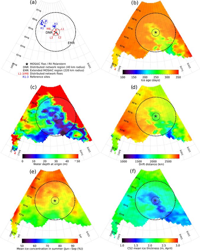
T. Krumpen et al.: The MOSAiC ice floe                                                                                                2175

Figure 1. Initial sea ice conditions in the MOSAiC study region on 25 September 2019, shortly before anchoring at the MOSAiC floe.
(a) Satellite-based sea ice concentration (source: University of Bremen). (b) Ship tracks of Polarstern (white) and Akademik Fedorov (black)
superimposed on a MODIS image (source: NASA) obtained on 22 September 2019. The red circle indicates the distributed network region
(DNR, 40 km radius). (c) Akademik Fedorov (right) and Polarstern (left) during bunkering procedure in thin ice, (d) Sentinel-1 SAR image
operated at C-band obtained on September 25 (source: ESA). The DN was mostly installed on the darker floes that correspond to older ice that
had survived the summer (residual ice). The position of the Central Observatory is marked by a black rectangle. (e) Close-up of the Central
Observatory based on a TerraSAR-X image (X-band) obtained on September 25 (source: DLR). The floe was initially 2.8 km × 3.8 km in
size and is characterised by a strongly deformed zone in the centre, called the “fortress”.

2     Material and methods                                              a combination of satellite-derived, low-resolution drift prod-
                                                                        ucts (Krumpen et al., 2019). The approach has also been ap-
2.1    Lagrangian sea ice trajectories                                  plied in a number of previous studies for the same purpose
                                                                        (Ricker et al., 2018; Damm et al., 2018; Peeken et al., 2018;
To determine the origin, pathways and thickness changes                 Krumpen et al., 2016 and others). In summary, IceTrack uses
of sea ice, as well as the atmospheric forcing acting on                a combination of three different publicly available ice drift
the ice cover, we use our Lagrangian drift analysis system              products for the tracking: (i) motion estimates based on a
called IceTrack that traces sea ice backward in time using              combination of scatterometer and radiometer data provided

https://doi.org/10.5194/tc-14-2173-2020                                                        The Cryosphere, 14, 2173–2187, 2020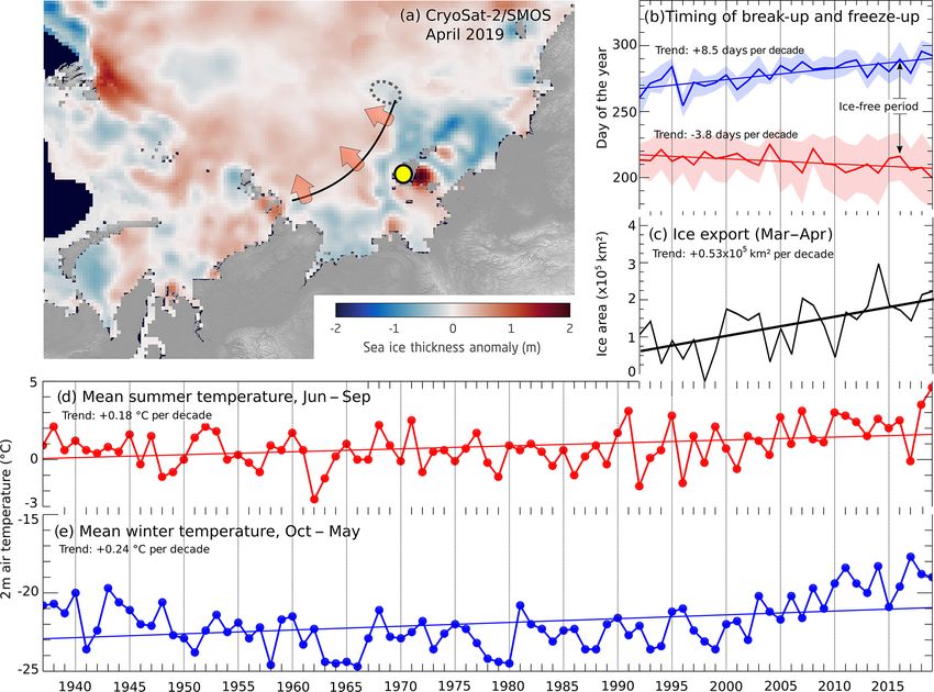
2176                                                                                  T. Krumpen et al.: The MOSAiC ice floe

by the Center for Satellite Exploitation and Research (CER-        counts for thermodynamic growth and melting as well as me-
SAT; Girard-Ardhuin and Ezraty, 2012), (ii) the OSI-405-c          chanical redistributions due to ridging (e.g. Thorndike et al.,
motion product from the Ocean and Sea Ice Satellite Ap-            1975; Lipscomb, 2001). For the purpose of this study, the me-
plication Facility (OSI SAF; Lavergne, 2016), and (iii) Po-        chanical aspect was disregarded in order to focus on thermo-
lar Pathfinder Daily Motion Vectors (v.4) from the National        dynamically grown level ice. At each time step, the growth
Snow and Ice Data Center (NSIDC; Tschudi et al., 2016).            and melt rates are derived from heat fluxes based on atmo-
The contributions of individual products to the used motion        spheric and oceanic forcing by solving conservation laws of
field are weighted based on their accuracies and availability      snow and ice enthalpy (e.g. be Bitz and Lipscomp, 1999).
which vary with seasons, years and study region. The Ice-          Every simulation began with open-ocean conditions. The at-
Track algorithm first checks for the availability of CERSAT        mospheric forcing was provided by NCEP reanalysis data
motion data within a predefined search range. CERSAT pro-          (Kanamitsu et al., 2002) and consisted of downward short-
vides the most consistent time series of motion vectors start-     and longwave radiation fluxes, surface air temperature and
ing from 1991 to present and has shown good performance            specific humidity, wind field, and precipitation. The oceanic
on the Siberian shelves (Rozman et al., 2011). During sum-         forcing, including sea surface temperature and salinity, was
mer months (June–August) when drift estimates from CER-            derived from a climatology based on hydrographic surveys
SAT are missing, motion information is bridged with OSI            carried out in the Laptev Sea (Janout et al., 2016), where
SAF (2012 to present). Prior to 2012, or if no valid OSI SAF       most of the ice originated.
motion vector is available within the search range, NSIDC
data are applied. The tracking approach works as follows:          2.3     Area flux estimates
ice in user-defined individual starting locations or positions
on a 25 km EASE2 grid is traced backward in time on a daily        To investigate the impact of winter sea ice dynamics on the
basis. Tracking is discontinued if (a) the tracked ice reaches     summer ice cover, we calculate monthly sea ice area fluxes
the coastline or fast ice edge or (b) the ice concentration at a   through the northern boundary of the Laptev Sea for the win-
specific location along the backward trajectory drops below        ter season from March to April (1992–2019). The gate is lo-
40 % and we assume the ice to be formed.                           cated between 110 and 160◦ E at 77.5◦ N (black line with
                                                                   arrows in Fig. 2a). The flux calculations follow the approach
2.2     Auxiliary data extracted along the track                   of Ricker et al. (2018), who estimated volume fluxes through
                                                                   the Fram Strait. For ice concentration, we use the CERSAT
2.2.1    Ice concentration and water depth                         product. For ice motion, we use merged products from CER-
                                                                   SAT that are based on radiometer and scatterometer data.
Ice concentration along the trajectories is provided by CER-       Figure 2c shows the total ice area export from March to April
SAT and based on 85 GHz SSM/I brightness temperatures.             of each winter, including a trend line plotted on top.
The CERSAT product makes use of the ARTIST Sea Ice
                                                                   2.4     Sea ice break-up and freeze-up
(ASI) algorithm and is available on a 12.5 km × 12.5 km grid
(Ezraty et al., 2007). Information on water depth was ob-
                                                                   The timing of sea ice break-up and freeze-up (Fig. 2b) was
tained from the International Bathymetry Chart of the Arctic
                                                                   estimated for each year based on CERSAT sea ice concen-
Ocean (IBCAO, Jakobsson et al., 2012).
                                                                   tration data for the region between 86◦ N, 100◦ E and 71◦ N,
                                                                   160◦ E. An ice-free grid point is defined as the first day in
2.2.2    Satellite-based and model-based sea ice thickness         a series of at least 10 d when ice concentration exceeds and
         estimates                                                 reaches zero (Janout et al., 2016).
The satellite-based sea ice thickness observations used in this    2.5     Field observations
study are based on the weekly merged CryoSat-2–SMOS sea
ice thickness product provided on a 25 km EASE2 grid by the        2.5.1    Snow and ice thickness measurements
AWI (Ricker et al., 2017). Weekly estimates from April were
then averaged in order to obtain monthly sea ice thickness         Ground-based electromagnetic (GEM) induction measure-
estimates for April 2019 (compare Fig. 2a).                        ments of ice thickness were obtained on five different resid-
   In addition to satellite-based mean thickness estimates, the    ual ice floes between 1 and 7 October: four floes were located
level ice thickness was computed along the Lagrangian drift        in the vicinity of the CO (∼ 15 km) and part of the DN (see
trajectories by means of the one-dimensional thermodynamic         Fig. 3a, L1-L3, M8). The fifth floe was positioned outside the
model Icepack (see CICE Consortium, 2020) that drifted             DN and will hereafter be called Reference Site R1.
with the ice. The single-column model describes the seasonal          The GEM was mounted on a plastic sledge and pulled
evolution of thickness distribution for a single floe from an      across the snow surface. The most frequently occurring ice
initial ice thickness. It uses an approach combining seven ice     thickness, the mode of the distribution (compare Fig. 6), rep-
categories and seven layers (only one layer of snow) and ac-       resents level ice thickness and is the result of winter accretion

The Cryosphere, 14, 2173–2187, 2020                                                    https://doi.org/10.5194/tc-14-2173-2020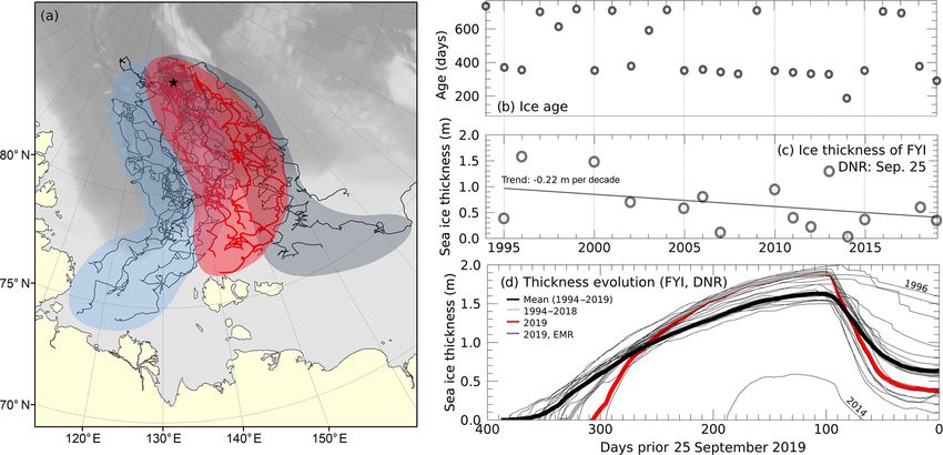
T. Krumpen et al.: The MOSAiC ice floe                                                                                                      2177

Figure 2. Summary of various processes that affected ice formation in the Laptev Sea and the East Siberian Sea in winter 2018/2019:
(a) CryoSat-2–SMOS sea ice thickness anomaly at the end of the winter (April 2019 minus April 2010–2018) in the eastern Eurasian Arctic.
A zone of thinner ice was present prior to the onset of melting along the coastline. The ice field in which the MOSAiC expedition was set up 5
months later is marked by a dotted line. (b) Estimate of the onset of break-up (red line) and freeze-up (blue line) with their standard deviations
and trends between 86◦ N, 100◦ E and 71◦ N, 160◦ E. (c) Satellite-based late winter (March–April) ice area export through a “gate” spanning
from 110 to 160◦ E at 77.5◦ N. A trend line is plotted on top. In (a), the gate is depicted as a solid black line. (d, e) Air temperatures (2 m)
recorded at Kotelny meteorological station (yellow circle in a) between 1935 and 2019 in the summer (red line) and winter months (blue
line). All trends provided in this graph are significant at a 95 % confidence level.

and summer ablation. According to Haas and Eicken (2001),                     While searching for a suitable floe for the CO, two addi-
a comparison of GEM measurements performed in the cen-                     tional regions were visited (see Fig. 3a, R2 and R3), each
tral Arctic during summer months with drill-hole data indi-                consisting of a collection of smaller floes. Here, manual ice
cate that the accuracy of the induction measurements is better             and snow thickness measurements were taken on the level ice
than 0.05–0.10 m and that the method is well suited for high-              with a drill, measuring stick, and thickness gauge.
resolution thickness profiling. For further details on the data               Table 1 summarises the mean and modal thickness of sea
processing and handling, we refer Hunkeler et al. (2016).                  ice and snow for all individual sampling sites.
   It is important to note here that electromagnetic sounding
only yields the total ice thickness (snow thickness plus sea               2.5.2    Ice coring
ice thickness). Therefore the snow surface layer thickness has
to be measured independently to yield ice thickness. Snow                  Ice cores were taken at all the L sites (Fig. 3a) with a stan-
thickness measurements on L1–L3 and M8 were obtained ev-                   dard 9 cm Kovacs ice corer. At L1, four cores were collected.
ery 2–5 m along the GEM tracks with a magnaprobe (Snow                     At L2, three cores were taken from level ice and three cores
Hydro, Fairbanks, AK, USA). At R1, manual snow thickness                   from a ridge at different surface elevations. At L3, three cores
measurements were taken at randomly selected locations. Af-                were extracted from level ice and three cores at the lower
ter GEM and magnaprobe measurements were converted to a                    relief area of a ridge. Within the MOSAiC central floe, ice
drift- and rotation-corrected coordinate system using a GPS                coring took place at several sites on a weekly basis, but only
reference station, sea ice thickness was calculated by sub-                the sediment-laden sea ice observed at one of the residual
tracting total ice thickness from snow thickness.                          ice stations is discussed in this paper. The ice cores were
                                                                           sectioned into 10 cm samples, melted, and then filtered for

https://doi.org/10.5194/tc-14-2173-2020                                                            The Cryosphere, 14, 2173–2187, 2020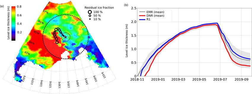
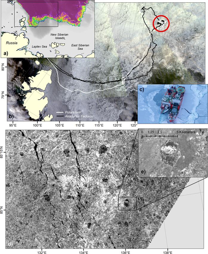
2178                                                                                          T. Krumpen et al.: The MOSAiC ice floe

Figure 3. Results of Lagrangian sea ice backward tracking (see Methods). (a) Starting point of the MOSAiC expedition (black star: position
of the Central Observatory), the spatial extent of the investigation areas defined in this paper (DNR and EMR), and the reference sites where
additional ice and snow thickness measurements were obtained. (b) Sea ice age at the start of the MOSAiC expedition on 25 September
according to Lagrangian tracking. (c) Water depth at the ice formation site for each tracking position. (d) Average distance of sea ice
travelled from its formation site to its position on 25 September. (e) Sea ice concentration for each individual point, averaged over the first
3 months (June–September) of tracking along its trajectory. (f) CryoSat-2 ice thickness estimates in late April, along the trajectory of each
point.

sediments using 0.45 µm filters. At all sampling sites, paral-            biogeochemical conditions from the initial ice formation.
lel cores were taken and stored at −20 ◦ C for future methane             This further demonstrates the importance of understanding
concentration and isotope analysis. Since the MOSAiC floes                the history of the MOSAiC floe for future studies.
may originate from methane supersaturated seawater near the
Siberian coast, some of the residual ice may contain relict

The Cryosphere, 14, 2173–2187, 2020                                                            https://doi.org/10.5194/tc-14-2173-2020
T. Krumpen et al.: The MOSAiC ice floe                                                                                                2179

Table 1. Ice and snow thickness observations obtained on various residual ice floes in the immediate vicinity (grey, L1–L3, M8) and extended
surroundings (R1–R3) of the Central Observatory. The positions of the sites are shown in Fig. 3a. Sample unit indicates either the distance
covered by instruments like GEM/magnaprobe (in kilometres) or the number (n) of individual measurements that were performed manually.
Numbers in parentheses provide the standard deviation.

                                                 Ice thickness (m)                  Snow thickness (m)            Total ice thickness (m)
    Site    Sampling device       Date         Mean     Mode     Samples           Mean     Modal     Samples     Mean             Mode
    L1      GEM/magnaprobe       5 Oct    0.86 (0.66)     0.43       8.7 km   0.10 (0.04)     0.07    n = 659      0.96              0.5
    L2      GEM/magnaprobe       7 Oct    0.67 (0.54)     0.33       9.6 km   0.11 (0.04)     0.08    n = 519      0.78             0.41
    L3      GEM/magnaprobe       9 Oct     1.0 (0.81)     0.31       7.9 km   0.11 (0.05)     0.06    n = 799      1.11             0.37
    M8      GEM/magnaprobe      11 Oct    0.76 (0.75)     0.35       1.2 km   0.09 (0.04)     0.06    n = 385      0.85             0.41
    R1      GEM/magnaprobe       1 Oct    0.85 (0.47)     0.62        21 km   0.11 (0.04)     0.09     n = 86      0.96             0.71
    R2      Manual               2 Oct     0.55 (0.1)     0.60       n = 38          0.18     0.18     n = 38      0.73             0.78
    R3      Manual               2 Oct    0.61 (0.17)     0.70       n = 20          0.06     0.06     n = 20      0.67             0.76

2.5.3      Ice observations from the bridge                              fect on the ice cover. During late winter months dominated
                                                                         by an offshore-directed drift component, newly formed ice
On board Akademik Fedorov, visual ice observations were                  areas are larger and remain comparatively thin and there-
carried out from the bridge by a group of three specially                fore melt more rapidly once temperatures rise above freezing.
trained ice observers. Detailed descriptions of the method-              This feedback mechanism is even more pronounced when
ology and protocols applied are provided in Alekseeva et                 temperatures at the end of winter are unusually high. Fig-
al. (2019) and AARI (2011), all congruent to the WMO Sea                 ure 2 summarises the conditions and processes that shaped
Ice Nomenclature (2017). Continuous 24 h ice observations                ice formation in the Laptev Sea and East Siberian Sea in win-
were available from 28 September (approaching R1) to 3 Oc-               ter 2018/2019. Satellite-based estimates of offshore-directed
tober (approaching the DN). The observations included vi-                sea ice area transport between March and April are shown
sual descriptions of the ice cover’s main characteristics, i.e.          in Fig. 2c (1992–2019, from 110 to 160◦ E at 77.5◦ N).
total concentration and partial concentrations and forms of              Late winter flux estimates indicate that the sea ice advec-
the encountered stages of ice development, hummock and                   tion away from the Siberian shelves towards the central Arc-
ridge concentration, melting stage, and sizes and orientations           tic was approximately 70 % higher (2.32 × 10⁵ km2 ) in 2019
of fractures and leads. In this paper, we will use the observed          than the long-term mean annual rate (∼ 1.36 × 10⁵ km2 ).
(within the limits of horizontal visibility) residual ice frac-          Following Krumpen et al. (2013), the strong positive trend
tion along the ship’s track (see Fig. 5). Data were resampled            (+0.53 × 10⁵ km2 per decade) in late winter ice area export
to an hourly interval.                                                   is associated with an increasing drift speed as a result of thin-
                                                                         ning ice cover and a rapid loss of thick multi-year ice. As a
                                                                         consequence of the intensified ice advection shortly before
3     Results and discussion                                             spring break, satellite-based sea ice thickness observations
                                                                         (Fig. 2a) show negative thickness anomalies throughout the
3.1     Sea ice retreat in summer 2019: preconditioning                  entire coastal zones of the East Siberian Sea and the Laptev
        processes                                                        Sea in April 2019, except for the southern half of the area
                                                                         around the New Siberian Islands.
Sea ice retreat during the melting period in the Laptev Sea                 Ocean-driven preconditioning mechanisms are less well
and East Siberian Sea is the result of atmospheric and oceanic           understood. However, there is indication that enhanced win-
processes and regional feedback mechanisms acting on the                 ter ventilation of the ocean can reduce sea ice formation in
ice cover, in both winter and summer. In the following, we               this area at a rate now comparable to losses from atmospheric
will briefly review the sea ice conditions on the Siberian               thermodynamic forcing (Polyakov et al., 2017). Observations
Shelf seas prior to the start of the expedition and the main             carried out in the eastern Eurasian Basin have shown that
preconditioning mechanisms that contributed to the north-                weakening of the halocline and shoaling of intermediate-
ward retreat of the ice edge in 2019. In this regard, our focus          depth Atlantic water layer result in heat flux equivalent to 40–
is on the atmospherically driven processes, since results from           54 cm reductions in ice growth in 2013/2014 and 2014/2015.
oceanographic surveys are not yet available.                                In addition, anomalously high temperatures during the
   Ice dynamics and ice export in winter are important pre-              winter months can further reduce the growth of first-year ice
conditioning mechanisms for the ice retreat in summer.                   (FYI), resulting in thinner ice cover at the end of the win-
Itkin and Krumpen (2017) observed that enhanced offshore-                ter (Ricker et al., 2017). According to NCEP reanalysis data
directed transport of sea ice in late winter has a thinning ef-

https://doi.org/10.5194/tc-14-2173-2020                                                        The Cryosphere, 14, 2173–2187, 2020
2180 T. Krumpen et al.: The MOSAiC ice floe
(Fig. S1, Supplement) and observations from the Kotelny the EMR shortly before MOSAiC’s starting date. Figure 3b
meteorological station (Fig. 2a, yellow circle), the tempera- shows the age of the sea ice within the EMR on 25 Septem-
tures during the ice growth phase (October 2018–May 2019) ber. Based on the backtracking analysis, the EMR’s resid-
were elevated: reanalysis data show positive temperature ual ice had an average age of 318 d and was formed on
anomalies of 3 ◦ C in comparison to the 1981–2010 climatol- 11 November 2018 (±15 d). Second-year (SYI) or multi-year
ogy, and records at Kotelny show significantly higher temper- ice (MYI) was not found, either from tracking or from scat-
atures than those at the beginning of the instrumental record terometer data. Most of the residual ice was originally pro-
(Fig. 2e). In particular, temperatures at the end of the win- duced during or shortly after the freeze-up in polynyas (or
ter are unusually high. If this coincides, as described above, elsewhere on the shallow Siberian shelves) (Fig. 3c), featur-
with periods of strong offshore-directed winds, the formation ing water depths of less than 30 m. Only the ice at the far
of new ice in coastal areas is reduced, which favours early eastern and northern edges of the EMR originated from re-
melting of the ice cover in spring (Fig. S2, Supplement). gions with a water depth exceeding 50 m. From the time of its
The subsequent temperature anomalies in spring and sum- formation to 25 September, the EMR ice had travelled an av-
mer 2019 were even more pronounced. During the summer erage distance of approximately 2440 km (±205 km, Fig. 3d)
months, Kotelny meteorological monitoring station recorded and experienced low ice concentrations between June and
the highest mean temperatures since the beginning of record- September 2019 (Fig. 3e). Hence, the residual ice encoun-
keeping (Fig. 2d), and the reanalysis data indicate a pos- tered after our arrival on site was severely weathered, and
itive anomaly of 2.5◦ on the Siberian shelves and in ad- bridge observations indicated that a large fraction was melted
jacent northern regions (Fig. S1, Supplement). The rapidly completely during summer months. Residual ice that sur-
rising temperatures in spring accelerated the melting of the vived was characterised by frozen-over melt ponds with a
ice cover, which was extremely thin to begin with (Fig. 2a). < 10 cm deep layer of fresh snow. Based on visual observa-
This resulted in the earliest ice break-up ever observed (com- tion, melt pond fraction was 70 %–80 % in the undeformed
pare Fig. 2b, red line) and rapid northward retreat of the ice areas, and the bottom layer experienced internal melting.
ice edge, which exposed surface waters to direct solar heat- According to ice coring, only the top 30 cm of ice was solid.
ing. Consequently, summer (August 2019) sea surface tem- Because both ships only reached the target region after the
peratures south of the MOSAiC starting area were approx- freeze-up had begun, large expanses of previously open wa-
imately 2–4 ◦ C higher than the 1982–2010 mean (Timmer- ter were now covered with new ice.
mans and Ladd, 2019), such that wind events that force ice Based on the backtracking analysis, the floes selected for
floes back into warm waters could have caused additional the Central Observatory and the DN were located in a zone of
ice melt (Steele and Ermold, 2015). Moreover, the intensive comparatively young ice that formed roughly 3 weeks later
warming of the upper ocean (Janout et al., 2016) caused a than the ice within the EMR (Fig. 3b, early December 2018)
delay in the autumnal freeze-up of sea ice (Fig. 2b, blue line) and originated from a shallow (Fig. 3c) region closer to its lo-
and resulted in large parts of the marginal seas remaining ice- cation on 25 September (Fig. 3d, 2240 km). Figure 4a shows
free for up to 93 d. This means that the MOSAiC expedition the trajectories obtained for the centre of the DNR (the po-
started immediately after the longest recorded ice-free period sition of the CO, red line) and four adjacent positions at a
in the region. distance of 25 km (grey lines). Information on water depths
and ice concentration along the central trajectory is provided
3.2 Sea ice origin and initial conditions in in Fig. 4b, c. The trajectories indicate that the ice inside the
September 2019 DNR was formed in a polynya event on 5 December 2018,
north of the New Siberian Islands in water that was less than
In this section we describe the predominant ice conditions 10 m deep. An eastward ice drift then transported the newly
at the beginning of MOSAiC, in both the ship’s immediate formed ice along the shallow shelf, until it reached deeper
vicinity and its extended surroundings. The latter encompass water in early February 2019. Ice cores collected at various
the area within a 220 km radius of Polarstern and will here- points in the DN and on the CO confirm that the DNR ice
after be referred to as the extended MOSAiC region (EMR; originated in the shallow Siberian shelves, since some of the
see Fig. 3a). A radius was selected to include various ice cores contained sediment inclusions of sandy silt in the up-
types, which differ in terms of their provenance (i.e. ori- permost 50 cm (Fig. 4c, d). Though the quantities were small
gin) and/or age. The EMR includes both the ice edge to the in most cases, these inclusions can only be found on the shal-
south and thicker and more stable pack ice to the north. The low Siberian Arctic shelves with average water depths of less
ship’s immediate vicinity (distributed network region, DNR) than 30 m (Sherwood, 2000; Wegner et al., 2017). There, par-
includes the DN and has a radius of 40 km. We will first de- ticulate matter and organisms are incorporated into the newly
scribe the ice conditions in the EMR, before turning our at- formed ice by suspension freezing (Eicken et al., 2000) or, to
tention to the DNR. a smaller degree, by grounded sea ice pressure ridges plough-
Once the MOSAiC floe had been chosen, we applied a ing through the sea floor (Darby et al., 2011). A detailed
tracking tool (see Methods) to the residual ice that was in
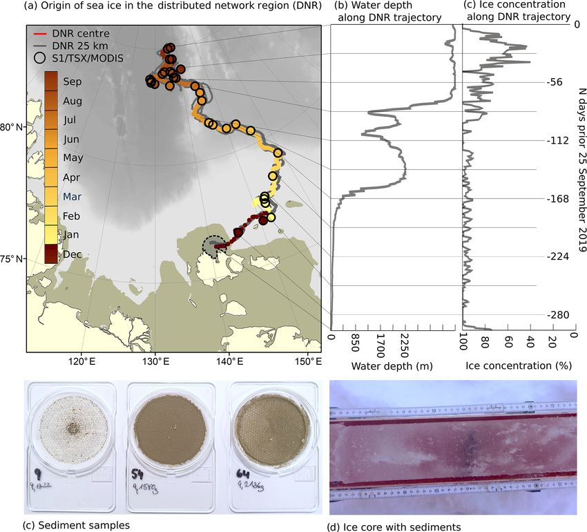
The Cryosphere, 14, 2173–2187, 2020 https://doi.org/10.5194/tc-14-2173-2020T. Krumpen et al.: The MOSAiC ice floe 2181 Figure 4. (a) Lagrangian backward trajectories (see Methods) of the DNR. The multicoloured trajectory line, with colour corresponding to the month of year, indicates the centre of the DNR (Central Observatory). The dashed circle provides the confidence bound of the ice origin. The grey lines provide additional trajectories for four points in the DNR at a distance of 25 km. Derived trajectories were verified by a manual tracking of the Central Observatory based on Sentinel-1, TerraSAR-X and MODIS (multicoloured circles). The bathymetry is shown in the background. Brownish zones near the coast indicate shallow-water areas of less then 30 m water depth. Panels (b) and (c) show water depth (m) and ice concentration (%) along the trajectory of the Central Observatory. (c) Sediment samples obtained from 10 cm ice core sections at L1 (left: level ice, 20–30 cm depth), L2 (middle: ridged/rafted ice, 243–253 cm depth, processed depth accounting for gaps in the core) and the central floe (right: ridged/rafted area at 49–59 cm depth). (d) Ice core taken at the central floe (c, right) with a sediment layer. chemical analysis of these trapped sediments will be con- tent in the atmosphere further reduce accuracy of low- ducted at a later point in time. resolution motion products (Sumata et al., 2014), IceTrack The validity and reliability of Lagrangian drift studies de- uses the OSI SAF motion product to bridge the lack of CER- pend on the accuracy of the applied sea ice motion product. SAT data. To quantify uncertainties of sea ice trajectories on In this study, we primarily use the CERSAT drift dataset a larger temporal and spatial scale, we reconstructed the path- because it provides the most consistent time series of mo- ways of drifting buoys using IceTrack. For this purpose, we tion vectors starting from 1991 to present (see Methods). selected 10 buoys that had survived a full summer and winter Comparisons with buoys and high-resolution SAR images in the Arctic. Their drift was then reproduced from October indicate that in particular during winter months, when the onwards in a backward direction over 12 months. Figure S3 atmospheric moisture content is low and surface melt pro- (Supplement) shows the deviation between actual and virtual cesses are absent, the quality of motion products from low- tracks, which is rather small (60 ± 24 km after 320 d) and in resolution satellites is high (Sumata et al., 2014; Krumpen et an acceptable range. The maximum deviation between real al., 2019). Restrictions may arise from the coarse resolution and virtual buoys gives a measure of the largest possible error of the sensors in near-shore regions characterised by a com- that can occur when determining the ice origin. After 320 d plex coastline, extensive fast-ice areas, and polynyas (Roz- it is around 105 km. The confidence bound is shown in Fig. 4 man et al., 2011). During summer months (June–August), as an ellipsoid (dashed line). No significant differences in sea when strong surface melt processes and high moisture con- ice pathways and source areas were observed when repeating https://doi.org/10.5194/tc-14-2173-2020 The Cryosphere, 14, 2173–2187, 2020
2182                                                                                    T. Krumpen et al.: The MOSAiC ice floe

Figure 5. (a) Level ice thickness on 25 September 2019 simulated with a thermodynamic model (see Methods). The percentage of residual
ice observed along the course of Akademik Fedorov (black circles) is superimposed. (b) Growth and melt of level ice in the EMR, DNR and
at R1 (cf. Fig. 3a).

the tracking experiment using different combinations of mo-           ence; results not shown here). Nevertheless, the decrease in
tion products, or higher and lower ice concentration thresh-          ice thickness toward the DNR is clearly recognisable in both
olds.                                                                 models and is in agreement with direct field observations:
   Note that we originally planned to trace the provenance            Fig. 6 shows the results of the GEM ice thickness measure-
of the MOSAiC floe using high-resolution satellite data               ments carried out on four floes in the distributed network
(Sentinel-1, TerraSAR-X and MODIS). However, only spo-                (L1–L3 and M8) and compares them with measurements
radic high-resolution images of the region were available,            taken on R1. The measured difference in modal ice thick-
and the combination of low summertime sea ice concen-                 nesses (without snow) between R1 and the DNR was 0.3 m
tration and high degree of cloud cover made it extremely              (R1: 0.5 m vs. DNR: 0.2 m). Higher ice thicknesses were also
difficult to manually track the exact position of individual          measured at R2 and R3 located farther to the north and west,
floes over an extended period of time. Nevertheless, the high-        which were reached by helicopter (Table 1, Methods).
resolution satellite data enabled us to track nearby large-scale         Visual observations made from the bridge of the Akademik
patterns such as shear zones or very prominent floes. Hence,          Fedorov as it travelled along the expedition route provided
we could at least determine the approximate location of the           further evidence for the presence of a thickness gradient be-
MOSAiC floe on individual images. The resulting estimates             tween the DNR and EMR. The percentage of residual ice
for the different positions of the CO (brown-yellow coloured          steadily dropped from nearly 90 % at R1 to 20 % at the DNR;
circles in Fig. 4a) correspond well to the computed trajecto-         conversely, the percentage of thin, newly formed ice rose
ries (red line in Fig. 4a), which lends increased confidence in       from 10 % to ca. 80 %. This indicates that, given its lower
our results.                                                          initial thickness at the end of the winter, some of the ice
   To calculate the ice thickness variability in the EMR and          in the DNR could have completely melted in summer. The
DNR at the start of MOSAiC (Fig. 5a) and the ice thickness            thickness gradient between the DNR and EMR is confirmed
evolution along the drift trajectories encountered by the ice         by CryoSat-2–SMOS measurements from the end of win-
in those regions (Fig. 5b), we used the results of a thermody-        ter 2018/2019. Already in April 2019, a negative thickness
namic model (see Methods). Results show that the residual             anomaly prevails at the later starting position of the drift ex-
ice in the DNR was not only younger and originated from a             periment (Figs. 2a and 3f).
different location than the ice in the surrounding EMR, but
it was also thinner: on 25 September, the averaged ice thick-         3.3   MOSAiC ice conditions compared to previous years
ness inside the EMR was 0.58 m (±0.27 m), while the thick-
ness of ice inside the DNR was 0.37 (±0.09 m), i.e. 36 %
                                                                      We showed that due to its younger age and different prove-
(0.21 m) less than in the EMR. To confirm model results,
                                                                      nance, the DNR ice was thinner than the surrounding ice.
we applied a second, simpler thermodynamic model devel-
                                                                      But the thicknesses measurements summarised in Fig. 6
oped by Thorndike (1992) and used in Peeken et al. (2018)
                                                                      and Table 1 are also much smaller than what was observed
and Krumpen et al. (2019). The model is chiefly based on
                                                                      by Haas and Eicken (2001) in the 1990s by similar GEM
air temperatures, assumes a constant ocean heat flux and em-
                                                                      and drill-hole measurements. They found late-summer modal
ploys snow climatology, but indicates the existence of similar
                                                                      FYI thicknesses between 1.25 m (1995), 1.75 m (1993), and
thickness gradients between the EMR and DNR (40 % differ-
                                                                      1.85 m (1996) in regions near or south of the MOSAiC study

The Cryosphere, 14, 2173–2187, 2020                                                       https://doi.org/10.5194/tc-14-2173-2020
T. Krumpen et al.: The MOSAiC ice floe 2183
Figure 6. Total (ice plus snow, a) and snow (b) thickness distribution of the floes located inside the DNR (L1-3, M8, red line) and at R1
(blue line; see Fig. 3a for positions). Ice thickness measurements were made with a ground-based electromagnetic (GEM) instrument pulled
across the ice on a sledge. Snow thickness measurements were made with a magnaprobe.
region, supporting the notion of exceptionally thin ice in the of April, followed by above-average melt. An in-depth anal-
MOSAiC starting region. In this section, we compare the ysis of the applied forcing data in the thermodynamic model
conditions we encountered at the end of September 2019 reveals that the intensified ice production is a consequence
with those of previous years by applying the combined of reduced precipitation rates in winter 2018/2019 (Fig. S4,
tracking–thermodynamics model to the period between 1994 Supplement).
and 2019. Figure 7a shows the history and variation in imag- Through a comparison with in situ data, we have shown
inary MOSAiC floe trajectories for the past 26 years. Track- above that the thermodynamic model is able to simulate
ing was performed backwards in time starting from the DNR regional differences in ice thickness. However, in order to
region on 25 September of each year. Results indicate that verify that the model is capable to reproduce the interan-
the climatological probability that DNR ice originates from nual variability correctly, model estimates require compari-
the New Siberian Islands, like in 2019, is about 25 % (red son to historical observational data from the past. Unfortu-
shaded area and tracks). From a climatological perspective, nately, field surveys in this exact location and that time of
it is usually more likely that the ice at the starting position has the year are scarce, but GEM ice thickness measurements in
its origin in the Laptev Sea (55 %, light blue shaded area). A the surroundings of the DNR between 84 and 86.5◦ N and
smaller part (∼ 20 %) typically comes from the East Siberian 100 and 150◦ E (compare Fig. 3) were obtained by Haas and
Sea (grey shaded area). The approximate age of the ice near Eicken (2001) during the ARK-12 cruise of Polarstern in
the starting point is around either 1 or 2 years (Fig. 7b), August 1996. The authors obtained around 37 km of thick-
with a tendency towards decreasing ice age. This tendency ness profile data at 5 m horizontal spacing. They found aver-
of decreasing ice age is evident from the frequency of SYI. age FYI modal thicknesses of ∼ 1.85 m, typical for SYI or
While SYI occurred in about 64 % of all years between 1992 even MYI in summer. The 1996 GEM measurements were
and 2004, it was already much less frequent during the past obtained 6 weeks earlier in the melt season (10 to 22 Au-
15 years (20 %, 2005–2019). gust 1996) inside the EMR area and south of it. In com-
Figure 7c displays the time series of September FYI thick- parison, the exceptionally thick September 1996 ice is re-
ness estimates in the DNR for the period between 1994 and produced by our thermodynamic model with 1.6 m in the
2019. In addition, Fig. 7d provides the annual cycle of DNR DNR (Fig. 7c). According to Haas and Eicken (2001), the
ice growth and melt. An overall decrease in residual ice relatively thick ice in 1996 was due to specific atmospheric
thickness between 1994 and 2019 is visible (trend: −0.22 m circulation conditions during summer, characterised by per-
per decade), which is subject to a high interannual variability sistent low sea level pressure over the central Arctic. This
and therefore not statistically significant. The DNR ice en- resulted in very weak surface melt and the absence of melt
countered in September 2019 can be classified as exception- ponds north of approximately 84◦ N in 1996. The model re-
ally thin over a longer period of time (Fig. 7c). However, for sults and forcing data for 1996 confirm that strongly reduced
the larger region of the EMR, ice thicknesses in September net shortwave fluxes led to a significant reduction in ice melt-
2019 agree well with the long-term average (Fig. 7d). Both ing during the summer months. Even in years dominated by
DNR and EMR ice shows above-average growth rates in win- strong melting processes, the model seems to realistically re-
ter 2018/2019 as well as above-average thicknesses at the end produce ice thickness: in winter 2013/2014, ice formed com-
https://doi.org/10.5194/tc-14-2173-2020 The Cryosphere, 14, 2173–2187, 20202184 T. Krumpen et al.: The MOSAiC ice floe
Figure 7. Ice origin, age and thickness of the DNR ice on 25 September between 1994 and 2019: (a) trajectories from the past 26 years
separated by the region of origin: (i) blue: Laptev Sea; (ii) red: region north of the New Siberian Islands; (iii) grey: East Siberian Sea.
(b) Age of the ice in the DNR region on 25 September of each year. (c) Thickness of DNR FYI based on a thermodynamic model (Methods).
(d) Annual cycle of FYI growth and melt.
paratively late in the season and melted completely during further delayed freeze-up and led to the longest ice-free pe-
summer (Fig. 7d). Satellite sea ice concentration data con- riod since the beginning of satellite observations.
firm that the DNR region and large parts of the EMR were Backward trajectories of sea ice present in the large EMR
ice-free already at the beginning of August 2014. If com- around Polarstern during the initial phase of the MOSAiC
bined with reliable trajectory and realistic forcing data, the drift experiment indicate that the majority of residual ice was
good agreement between the thermodynamic model and ob- formed shortly after freeze-up in 2018. In comparison, the
servations for the years 1996, 2014 and 2019 shows that the ice within the smaller DNR around Polarstern was 3 weeks
model can be used to study interannual variability of FYI younger and formed on the shallow shelves north of the New
thickness changes and the driving mechanisms behind them. Siberian Islands. Sediments discovered in ice cores confirm
contact of sea ice with shallow waters in an early phase of
growth. While in recent years the strong ice retreat in sum-
mer melts most of the shallow-water ice on its way to the cen-
4 Conclusion and implications for future studies tral Arctic Ocean (Krumpen et al., 2019), part of the resid-
ual ice encountered in the DNR has survived summer melt.
In this study, we investigate the initial ice conditions and pre- Therefore, besides the original goals, MOSAiC will also pro-
conditioning mechanisms at the start of the MOSAiC drift vide an excellent opportunity to better understand the role
experiment. Moreover, we evaluate how representative the of sea ice as a transport medium for climate-relevant gases,
ice within the distributed network region (DNR) is compared macronutrients, iron, organic matter, sediments and pollu-
to the experiment’s extended surroundings (extended MO- tants from shelf areas to the central Arctic Ocean and be-
SAiC region, EMR), and we question whether the ice en- yond. This is particularly important because with predicted
countered was unusually thin compared to past years. changes towards a seasonally ice-free ocean under climate
An analysis of satellite-based observations, reanalysis data change a complete cut-off of the long-range transport of ice-
and readings from the meteorological station Kotelny from rafted materials by the Transpolar Drift appears possible in
2019 indicates that sea ice retreat in the Siberian Shelf seas the future. By comparing transport rates of residual ice with
was strongly influenced by ice dynamics in late winter and newly formed ice on site, one can examine the impact a re-
unusually high temperatures in summer. A high offshore- duced long-range transport of sea ice has for the redistribu-
directed transport of sea ice shortly before the onset of spring tion of biogeochemical matter in the central Arctic Ocean.
resulted in unusually thin ice cover throughout the entire The application of the thermodynamic model reveals that
coastal zones of the marginal seas in April. Rapidly rising ice in the DNR is 36 % thinner than the surrounding ice due
temperatures with record temperatures in summer acceler- to its younger age and different provenance of origin. Dif-
ated the melting of the thin ice cover and caused the earliest ferences in modal ice thickness between outer areas (sites
break-up since 1992. Intensive warming of the upper ocean
The Cryosphere, 14, 2173–2187, 2020 https://doi.org/10.5194/tc-14-2173-2020T. Krumpen et al.: The MOSAiC ice floe 2185
R1–R3) and the DNR are also evident in direct field obser- Competing interests. The authors declare that they have no conflict
vations. It is therefore to be expected that the momentum of interest.
and energy transfer between the ocean and the atmosphere is
subject to strong spatial variations. Future studies will show
whether these regional differences can be reproduced using Acknowledgements. This work was carried out as part of the
high-resolution models and satellite data. Whether the ob- Russian-German Research Cooperation QUARCCS funded by the
served thickness gradients also influence ice dynamics in the German Ministry for Education and Research (BMBF) under grant
03F0777A and CATS under grant 63A0028B. Data used in this pa-
immediate and extended surroundings of the Central Obser-
per were produced as part of the international Multidisciplinary
vatory is another exciting research question, and a compari-
drifting Observatory for the Study of the Arctic Climate (MO-
son of the ice dynamics in the DNR and EMR derived from SAiC) with the tag MOSAiC20192020 (AWI_PS122_1 and AF-
satellite data is work in progress. However, we assume that MOSAiC-1_00). NCEP Reanalysis 2 data are made available by
the encountered regional differences will balance out during NOAA/OAR/ESRL PSD, Boulder, Colorado, USA, from their web-
the ice growth phase and thus reduce the spatial variability site at https://www.esrl.noaa.gov/psd/ (last access: 25 June 2020).
in ice dynamics over the course of the winter and over the The work on satellite remote sensing data was partly funded
course of the whole MOSAiC expedition. through the EU H2020 project SPICES (640161), the ESA Sea
The ice thickness in September 2019 can be classified as Ice CCI phase 1 and 2 (AO/1-6772/11/I-AM), and the Helmholtz
exceptionally thin when compared to the last 26 years. In PACES II (Polar regions And Coasts in the changing Earth System)
this sense, we might have already experienced the “new nor- and FRAM (FRontiers in Arctic marine Monitoring) programmes.
TerraSAR-X images were provided by the German Aerospace Cen-
mal” of Arctic conditions during the initial phase of MO-
ter (DLR) through TSX Science AO OCE3562. We thank the crew
SAiC, which might make future follow-up campaigns of this of the research vessels Akademik Fedorov and Polarstern and the
scale increasingly difficult. An only seasonally ice-covered helicopter company Naryan-Marsky for their great logistical sup-
Arctic with a reduced (or even cut-off) transport of ice-rafted port during the set-up of the MOSAiC experiment and participants
material by the Transpolar Drift will have strong implications of the Akademik Fedorov cruise and MOSAiC School for helping
for the redistribution of biogeochemical matter in the central hands.
Arctic Ocean, with consequences for the balance of climate-
relevant trace gases, primary production and biodiversity in
the Arctic Ocean. Financial support. This research has been supported by the Ger-
man Ministry for Education and Research (grant no. 03F0777A),
the German Ministry for Education and Research (grant no.
Code and data availability. All data are archived in the MOSAiC 63A0028B), the German Aerospace Center (grant no. AO
Central Storage (MCS) and will be available on PANGAEA after fi- OCE3562), the German Minsitry for Education and Research
nalisation of the respective datasets according to the MOSAiC data (MOSAiC20192020), the EU H2020 (grant no. 640161), and the
policy. The production of the merged CryoSat-SMOS sea ice thick- European Space Agency (grant no. AO/1-6772/11/I-AM).
ness data was funded by the ESA project SMOS & CryoSat-2 Sea
Ice Data Product Processing and Dissemination Service, and data The article processing charges for this open-access
was obtained from http://meereisportal.de (ftp://ftp.awi.de/sea_ice/ publication were covered by a Research
product/cryosat2_smos/v202/, Hendricks and Ricker, 2019). NCEP Centre of the Helmholtz Association.
Reanalysis 2 data are made available by NOAA/OAR/ESRL PSD,
Boulder, Colorado, USA, from their website at https://www.esrl.
noaa.gov/psd/ (NOAA, 2020). Review statement. This paper was edited by Yevgeny Aksenov and
reviewed by two anonymous referees.
Supplement. The supplement related to this article is available on-
line at: https://doi.org/10.5194/tc-14-2173-2020-supplement. References
AARI: Guidance to Special Shipborne Ice Observations, Technical
Author contributions. TK conceived the study and wrote the paper. Report, Arctic and Antarctic Research Insitute (AARI), Saint-
FB, FK, SH, JB, VS, LvA, CH, TR, RR, VS, ED, AT, JH and SuS Petersburg, Russia, 2011.
undertook the data analysis, developed the methods or contributed Alekseeva, T., Tikhonov, V., Frolov, S., Repina, I., Raev, M.,
to interpretation of results. Field observations (thickness of snow Sokolova, J., Sharkov, E., Afanasieva, E., and Serovetnikov,
and ice, bridge observations, ice cores, etc.) were made and pro- S.: Comparison of Arctic Sea Ice Concentration from the
cessed by VB, TP, AM, AT, MH, ES, NK, JR, JB, JH, MT and MA. NASA Team, ASI, and VASIA2 Algorithms with Sum-
All authors commented on the manuscript mer and Winter Ship Data, Remote Sensing, 11, 2481,
https://doi.org/h10.3390/rs11212481, 2019.
Bitz, C. M. and Lipscomb, W. H.: An energy-conserving thermody-
namic sea ice model for climate study, J. Geophys. Res.-Oceans,
104, C7, https://doi.org/10.1029/1999JC900100, 1999.
https://doi.org/10.5194/tc-14-2173-2020 The Cryosphere, 14, 2173–2187, 20202186 T. Krumpen et al.: The MOSAiC ice floe CICE Consortium Icepack: Icepack version 1.1.0, Zenodo, trends in Laptev Sea ice outflow between 1992–2011, The https://doi.org/10.5281/zenodo.1213462, 2020. Cryosphere, 7, 349–363, https://doi.org/10.5194/tc-7-349-2013, Damm, E., Bauch, D., Krumpen, T., Rabe, B., Korhonen, M., 2013. Vinogradova, E., and Uhlig, C.: The Transpolar Drift conveys Krumpen, T. and Sokolov, V.: The Expedition AF122/1 : Setting methane from the Siberian Shelf to the central Arctic Ocean, up the MOSAiC Distributed Network in October 2019 with Re- Sci. Rep., 8, 4515, https://doi.org/10.1038/s41598-018-22801-z, search Vessel AKADEMIK FEDOROV, Berichte zur Polar- und 2018. Meeresforschung = Reports on polar and marine research, Bre- Darby, D. A., Myers, W. B., Jakobsson, M., and Rigor, I.: Modern merhaven, Alfred Wegener Institute for Polar and Marine Re- dirty sea ice characteristics and sources: The role of anchor ice, search, 744 , 119 pp., https://doi.org/10.2312/BzPM_0744_2020, J. Geophys. Res.-Oceans, 116, 2156–2202, 2011. 2020. Eicken, H., Koatschek, J., Lindemann, F., Dmitrenko, I., Freitag, J., Krumpen, T., Gerdes, R., Haas, C., Hendricks, S., Herber, A., Se- and Kassens, H.: A key source area and constraints on entrain- lyuzhenok, V., Smedsrud, L., and Spreen, G.: Recent summer sea ment for basin-scale sediment transport by Arctic sea ice, Geo- ice thickness surveys in Fram Strait and associated ice volume phys. Res. Lett., 27, 13, https://doi.org/10.1029/1999GL011132, fluxes, The Cryosphere, 10, 523–534, https://doi.org/10.5194/tc- 2000. 10-523-2016, 2016. Ezraty, R., Girard-Ardhuin, F., Piolle, J. F., Kaleschke, L., Heygster, Krumpen, T., Belter, J., Boetius, A., Damm, E., Haas, C., Hen- G.: Arctic and Antarctic Sea Ice Concentration and Arctic Sea Ice dricks, S., Nicolaus, M., Nöthig, E. M. , Paul, S., Peeken, I., Drift Estimated from Special Sensor Microwave Data, Techni- Ricker, R., and Stein, R.: Arctic warming interrupts the Transpo- cal Report, Departement d’Oceanographie Physique et Spatiale, lar Drift and affects longrange transport of sea ice and ice-rafted IFREMER, Brest, France, 2007. matter, Sci. Rep., 9, 5459, https://doi.org/10.1038/s41598-019- Girard-Ardhuin, F. and Ezraty, R.: Enhanced arctic sea ice drift 41456-y, 2019. estimation merging radiometer and scatterometer data, IEEE T. Lavergne, T.: Validation and Monitoring of the OSI SAF Low Res- Geosci. Remote., 50, 2639–2648, 2012. olution Sea Ice Drift Product (v5), Technical Report, The EU- Haas, C. and Eicken, J.: Interannual variability of summer sea ice METSAT Network of Satellite Application Facilities, July 2016 thickness in the Siberian and central Arctic under different atmo- Lipscomb, W. H.: Remapping the thickness distribution in sea ice spheric circulation regimes, J. Geophys. Res., 106, 4449–4462, models, J. Geophys. Res.-Oceans, 106, 13989–14000, 2001. 2001. NOAA: NCEP Reanalysis 2 data, available at: https://www.esrl. Hendricks, S. and Ricker, R.: Product User Guide & Algo- noaa.gov/psd/, last access: 25 June 2020 rithm Specification: AWI CryoSat-2 Sea Ice Thickness (version Polyakov, I. V., Pnyushkov, A. V., Alkire, M. B., Ashik, I. M., Bau- 2.2), available at: https://epic.awi.de/id/eprint/50033/ (last ac- mann, T. M., Carmack, E. C., Goszczko, I., Guthrie,J., Ivanov, V. cess: 25 June 2020), 2019. V., Kanzow, T., Krishfield, R., Kwok, R.,Sundfjord, A., Morison, Hunkeler, P., Hoppmann, M., Hendricks, S., Kalscheuer, T., and J., Rember, R., and Yulin, A.: Greater role for Atlantic inflows on Gerdes, R.: A glimpse beneath Antarctic sea ice: platelet-layer sea-ice loss in the Eurasian Basin of the Arctic Ocean, Science, from multi-frequency electromagnetic induction sounding, Geo- 6335, 285–291, https://doi.org/10.1126/science.aai8204, 2017. phys. Res. Lett., 43, 1, https://doi.org/10.1002/2015GL065074, Peeken, I., Primpke, S, Beyer, B., Guetermann, J., Katlein, 2016. C., Krumpen, T., Bergmann, M., Hehemann, L., and Gerdts, Itkin, P. and Krumpen, T.: Winter sea ice export from the Laptev Sea G.: Arctic sea ice is an important temporal sink and preconditions the local summer sea ice cover and fast ice decay, means of transport for microplastic, Nat. Commun., 9, 1509, The Cryosphere, 11, 2383–2391, https://doi.org/10.5194/tc-11- https://doi.org/10.1038/s41467-018-03825-5, 2018. 2383-2017, 2017. Ricker, R., Hendricks, S., Kaleschke, L., Tian-Kunze, X., King, J., Jakobsson, M., Mayer, L., Coakley, B, Dowdeswell, J., Forbes, and Haas, C.: A weekly Arctic sea-ice thickness data record from S., Fridman, B., Hodnesdal, H., Noormets, R., Pedersen, R., merged CryoSat-2 and SMOS satellite data, The Cryosphere, 11, Rebesco, M., Schenke, H. W., Zarayskaya, Y., Accettella, D., 1607–1623, https://doi.org/10.5194/tc-11-1607-2017, 2017. Armstrong, A., Anderson, R. M., Bienhoff, P., Camerlenghi, Ricker, R., Girard-Ardhuin, F., Krumpen, T., and Lique, C.: A., Church, I., Edwards, M., Gardner, J., Hall, J., Hell, B., Satellite-derived sea ice export and its impact on Arc- Hestvik, O., Kristoffersen, Y., Marcussen, C., Mohammad, tic ice mass balance, The Cryosphere, 12, 3017–3032, R., Mosher, D., Nghiem, S., Pedrosa, M., Travaglini, P., and https://doi.org/10.5194/tc-12-3017-2018, 2018. Weatherall, P.: The International Bathymetric Chart of the Arctic Rozman, P., Hoelemann, J., Krumpen, T., Gerdes, R., Koeberle, Ocean (IBCAO) Version 3.0, Geophys. Res. Lett., 39, L12609, C., Lavergne, T., and Adams, S.: Validating satellite derived https://doi.org/10.1029/2012GL052219, 2012. and modelled sea-ice drift in the Laptev Sea with in situ mea- Janout, M., Hölemann, Waite, A. M., Krumpen, T., Appen, W. J., surements from the winter of 2007/08, Polar Res., 30, 7218, and Martynov, F.: Sea-ice retreat controls timing of summer https://doi.org/10.3402/polar.v30i0.7218, 2011. plankton blooms in the Eastern Arctic Ocean, Geophys. Res. Sherwood, C. R.: Numerical model of frazil ice and suspended sed- Lett., 43, 24, https://doi.org/10.1002/2016GL071232, 2016. iment concentrations and formation of sediment laden ice in the Kanamitsu, M., Ebisuzaki, W., Woollen, J., Yang, S. K., Hnilo, J. J., Kara Sea, J. Geophys. Res.-Oceans, 105, 14061–14080, 2000. Fiorinom M., and Potter, G., H.: NCEP-DOE AMIP-II Reanaly- Steele, M. and Ermold, W.: Loitering of the retreating sea iceedge sis (R-2), B. Am. Meteorol. Soc., 83, 1631–1643, 2002. in the Arctic Seas, J. Geophys. Res., 120, 7699–7721, 2015. Krumpen, T., Janout, M., Hodges, K. I., Gerdes, R., Girard- Sumata, H., Lavergne, T., Girard-Ardhuin, F., Kimura, N., Tschudi, Ardhuin, F., Hölemann, J. A., and Willmes, S.: Variability and M. A., Kauker, F., Karcher, M., and Gerdes, R.: An intercompar- The Cryosphere, 14, 2173–2187, 2020 https://doi.org/10.5194/tc-14-2173-2020
You can also read