Wide-Field Lensing Mass Maps from DES Science Verification Data
←
→
Page content transcription
If your browser does not render page correctly, please read the page content below
Mon. Not. R. Astron. Soc. 000, 000–000 (0000)     Printed 12 April 2015   (MN LATEX style file v2.2)

Wide-Field Lensing Mass Maps from DES Science Verification Data

V. Vikram,1,2 C. Chang,3∗ B. Jain,2 D. Bacon,4 A. Amara,3 M. Becker,5,6
G. Bernstein,2 C. Bonnett,7 S. Bridle,8 D. Brout,2 M. Busha,5,6 J. Frieman,9,10
E. Gaztanaga,11 W. Hartley,3 M. Jarvis,2 T. Kacprzak,3 O. Lahav,12 B. Leistedt,12
H. Lin,10 P. Melchior,13,14 H. Peiris,12 E. Rozo,15 E. Rykoff,6,16 C. Sánchez, 7
E. Sheldon,17 M. Troxel,8 R. Wechsler,5,6,16 J. Zuntz,8 T. Abbott,18 F. B. Abdalla,12
R. Armstrong,2 M. Banerji,19,20 A. H. Bauer,11 A. Benoit-Lévy,12 E. Bertin,21
D. Brooks,12 E. Buckley-Geer,10 D. L. Burke,6,16 D. Capozzi,4 A. Carnero Rosell,22,23
M. Carrasco Kind,24,25 F. J. Castander,11 M. Crocce, 11 C. B. D’Andrea,4
L. N. da Costa,22,23 D. L. DePoy,26 S. Desai,27 H. T. Diehl,10 J. P. Dietrich,27,28
C. E Cunha,29 J. Estrada,10 A. E. Evrard,30 A. Fausti Neto,22 E. Fernandez,7
B. Flaugher,10 P. Fosalba,11 D. Gerdes,30 D. Gruen,31,32 R. A. Gruendl,24,25
K. Honscheid,13,14 D. James,18 S. Kent,10 K. Kuehn,33 N. Kuropatkin,10 T. S. Li,26
M. A. G. Maia,22,23 M. Makler,34 M. March,2 J. Marshall,26 Paul Martini,13,14
K. W. Merritt,10 C. J. Miller,30,35 R. Miquel,7,36 E. Neilsen,10 R. C. Nichol,4 B. Nord,10
R. Ogando,22,23 A. A. Plazas,17,37 A. K. Romer,38 A. Roodman,7,16 E. Sanchez,39
V. Scarpine,10 I. Sevilla,24,39 R. C. Smith,18 M. Soares-Santos,10 F. Sobreira,10,22
E. Suchyta,13,14 M. E. C. Swanson,25 G. Tarle,27 J. Thaler,24 D. Thomas,4,40
A. R. Walker,18 J. Weller27,28,31
∗ e-mail   address: chihway.chang@phys.ethz.ch

12 April 2015

                                        ABSTRACT
                                        Weak gravitational lensing allows one to reconstruct the spatial distribution of the projected
                                        mass density across the sky. These “mass maps” provide a powerful tool for studying cosmol-
                                        ogy as they probe both luminous and dark matter. In this paper, we present a weak lensing
                                        mass map reconstructed from shear measurements in a 139 deg2 area from the Dark Energy
                                        Survey (DES) Science Verification (SV) data overlapping with the South Pole Telescope sur-
                                        vey. We compare the distribution of mass with that of the foreground distribution of galaxies
                                        and clusters. The overdensities in the reconstructed map correlate well with the distribution of
                                        optically detected clusters. Cross-correlating the mass map with the foreground galaxies from
                                        the same DES SV data gives results consistent with mock catalogs that include the primary
                                        sources of statistical uncertainties in the galaxy, lensing, and photo-z catalogs. The statisti-
                                        cal significance of the cross-correlation is at the 6.8σ level with 20 arcminute smoothing. A
                                        major goal of this study is to investigate systematic effects arising from a variety of sources,
                                        including PSF and photo-z uncertainties. We make maps derived from twenty variables that
                                        may characterize systematics and find the principal components. We find that the contribution
                                        of systematics to the lensing mass maps is generally within measurement uncertainties. We
                                        test and validate our results with mock catalogs from N-body simulations. In this work, we
                                        analyze less than 3 % of the final area that will be mapped by the DES; the tools and analy-
                                        sis techniques developed in this paper can be applied to forthcoming larger datasets from the
                                        survey.
c 0000 RAS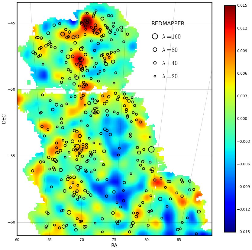
2      V. Vikram et al.
1   INTRODUCTION                                                          sities. The total area of the mass map in that work is similar to our
                                                                          dataset, though it was divided into four separate smaller fields.
Weak gravitational lensing is a powerful tool for cosmological stud-            The main goal of this paper is to construct a weak lensing mass
ies (see Bartelmann & Schneider 2001; Hoekstra & Jain 2008, for           map from a 139 deg2 area in the Dark Energy Survey1 (DES, The
detailed reviews). As light from distant galaxies passes through          Dark Energy Survey Collaboration 2005; Flaugher 2005) Science
the mass distribution in the Universe, its trajectory gets perturbed,     Verification (SV) data, which overlaps with the South Pole Tele-
causing the apparent galaxy shapes to be distorted. Weak lensing          scope survey (the SPT-E field). The SV data were recorded using
statistically measures this small distortion, or “shear”, for a large     the newly commissioned wide-field mosaic camera, the Dark En-
number of galaxies to infer the 3D matter distribution. This allows       ergy Camera (DECam; Diehl & Dark Energy Survey Collaboration
us to constrain cosmological parameters and study the distribution        2012; Flaugher et al. 2012; Flaugher & The Dark Energy Survey
of mass in the Universe.                                                  Collaboration submitted to A. J.) on the 4m Blanco telescope at
      Since its first discovery, the accuracy and statistical precision   the Cerro Tololo Inter-American Observatory (CTIO) in Chile. We
of weak lensing measurements have improved significantly (Van             cross correlate this reconstructed mass map with optically identi-
Waerbeke et al. 2000; Kaiser, Wilson & Luppino 2000; Bacon, Re-           fied structures such as galaxies and clusters of galaxies. This work
fregier & Ellis 2000; Hoekstra et al. 2006; Lin et al. 2012; Hey-         opens up several directions for future explorations with these mass
mans et al. 2012). Most of these previous studies constrain cos-          maps.
mology through N-point statistics of the shear signal (e.g. Bacon               This paper is organized as follows. In §2 we describe the theo-
et al. 2003; Jarvis et al. 2006; Semboloni et al. 2006; Fu et al.         retical foundation and methodology for constructing the mass maps
2014; Jee et al. 2013; Kilbinger et al. 2013). In this paper, how-        and galaxy density maps used in this paper. We then describe in
ever, we focus on generating two-dimensional wide-field projected         §3 the DES dataset used in this work, together with the simula-
mass maps from the measured shear (Van Waerbeke, Hinshaw &                tion used to interpret our results. In §4 we present the reconstructed
Murray 2014). These mass maps are particularly useful for view-           mass maps and discuss qualitatively the correlation of these maps
ing the non-Gaussian distribution of dark matter in a different way       with known foreground structures found via independent optical
than is possible with N-point statistics.                                 techniques. In §5, we quantify the wide-field mass-to-light corre-
                                                                          lation on different spatial scales using the full field. We show that
      Probing the dark matter distribution in the Universe is par-
                                                                          our results are consistent with expectations from simulations. In §6
ticularly important for several reasons. Based on the peak statis-
                                                                          we estimate the level of contamination by systematics in our results
tics from a mass map it is possible to identify dark matter halos
                                                                          from a wide range of sources. Finally, we conclude in §7.
and constrain cosmological parameters (e.g. Jain & Van Waerbeke
2000; Fosalba et al. 2008; Kratochvil, Haiman & May 2010; Bergé,
Amara & Réfrégier 2010). Mass maps also allow us to study the
connection between baryonic matter (both in stellar and gaseous           2     METHODOLOGY
forms) and dark matter (Van Waerbeke, Hinshaw & Murray 2014).             In this section we first briefly review the principles of weak lens-
This can be measured by cross correlating light maps and gas maps         ing in §2.1. Then, we describe the adopted mass reconstruction
with weak lensing mass maps. Correlation with light maps, which           method in §2.2. Finally in §2.3, we describe our method of gen-
can be constructed using observed galaxies, groups and clusters of        erating galaxy density maps. The galaxy density maps are used as
galaxies etc., can be used to constrain galaxy bias, the mass-to-light    independent mass tracers in this work to help confirm the signal
ratio, and the dependence of these statistics on redshift and envi-       measured in the weak lensing mass maps.
ronment (Amara et al. 2012; Jauzac et al. 2012; Shan et al. 2014;
Hwang et al. 2014). However, one needs to take caution when in-
terpreting the weak lensing mass maps, as the completeness and            2.1    Weak gravitational lensing
purity of structure detection via these maps is not very high due to
their noisy nature (White, van Waerbeke & Mackey 2002).                   When light from galaxies passes through a foreground mass dis-
                                                                          tribution, the resulting bending of light leads to the galaxy im-
      One other interesting application of the mass map is that it al-    ages being distorted (e.g. Bartelmann & Schneider 2001). This
lows us to identify large scale structures (both super-clusters and       phenomenon is called gravitational lensing. The local mapping be-
voids) which are otherwise difficult to find (e.g. Heymans et al.         tween the source (β ) and image (θ ) plane coordinates (aside from
2008). Characterizing the statistics of large structures can be a sen-    an overall displacement) can be described by the lens equation:
sitive probe of cosmological models. Structures with masses as
high or higher than clusters require special attention as the mas-                                β − β0 = A(θ )(θ − θ0 ),                    (1)
sive end of the halo mass function is very sensitive to the cosmol-
                                                                          where β0 and θ0 is the reference point in the source and the image
ogy (Bahcall & Fan 1998; Haiman, Mohr & Holder 2001; Holder,
                                                                          plane. A is the Jacobian of this mapping, given by
Haiman & Mohr 2001). These rare structures also allows us to con-
strain different theories of gravity (Knox, Song & Tyson 2006; Jain                                         1 − µ1    −µ2
                                                                                          A(θ ) = (1 − κ)                     ,           (2)
& Khoury 2010). In addition to the study of the largest assemblies                                           −µ2     1 + µ1
of mass, the study of number density of the largest voids allows
further tests of the ΛCDM model (e.g. Plionis & Basilakos 2002).          where κ is the convergence, µi = γi /(1 − κ) is the reduced shear
                                                                          and γi is the shear. i = 1, 2 refers to the 2D coordinates in the plane.
     Similar mass mapping technique as used in this paper has             The premultiplying factor (1 − κ) causes galaxy images to be di-
been previously applied to the Canada-France-Hawaii Telescope             lated or reduced in size, while the terms in the matrix cause dis-
Lensing Survey (CFHTLenS) as presented in Van Waerbeke et al.             tortion in the image shapes. Under the Born approximation, which
(2013). Their work demonstrated the potential scientific value of
these wide-field lensing mass maps, including measuring high-
order moments of the maps and cross-correlation with galaxy den-          1   http://www.darkenergysurvey.org

                                                                                                                c 0000 RAS, MNRAS 000, 000–000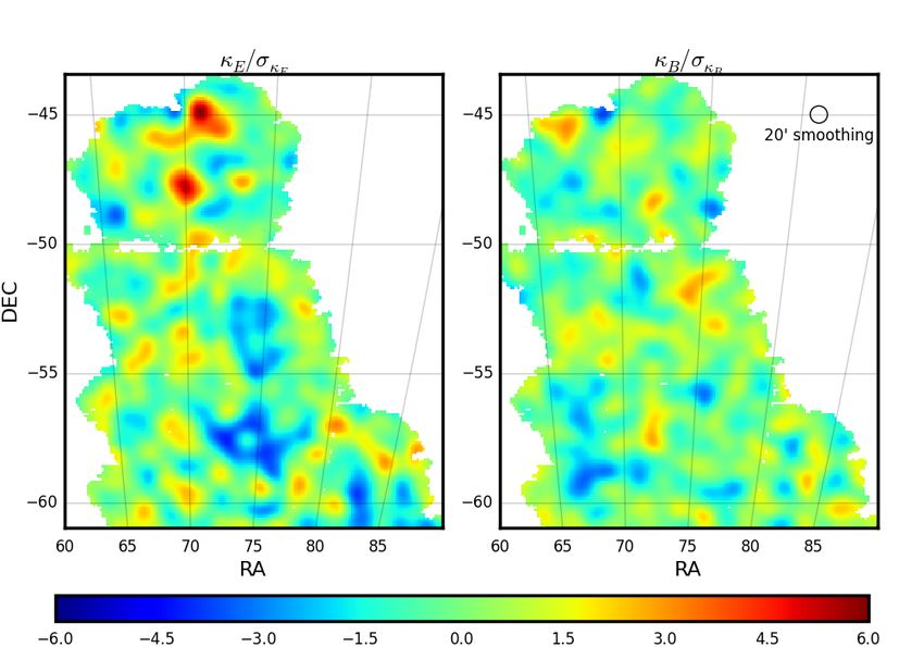
Wide Field Lensing Mass Maps from DES                         3
assumes that the deflection of the light rays due to the lensing effect              works as follows. The Fourier transform of the observed shear, γ̂,
is small, A is given by (e.g. Bartelmann & Schneider 2001)                           relates to the Fourier transform of the convergence, κ̂ through
                         Ai j (θ , r) = δi j − ψ,i j ,                         (3)                                 κ̂l = D∗l γ̂l ,                    (11)

where ψ is the lensing deflection potential, or projected gravita-
tional potential along the line of sight. For a spatially flat Universe,                                           l12 − l22 + 2il1 l2
                                                                                                            Dl =                       ,              (12)
it is given by the line of sight integral of the 3-dimensional gravita-                                                    |l|2
tional potential Φ,                                                                  where li are the Fourier counterparts for the angular coordinates θi ,
                                     Z r
                                               r − r0                                i = 1, 2 represent the two dimensions of sky coordinate. The above
                                           dr0        Φ θ , r0 ,

                ψ (θ , r) = −2                                                 (4)   equations hold true for l 6= 0. In practice we apply a sinusoidal pro-
                                      0          rr0
                                                                                     jection of sky with a reference point at RA=71.0 and then pixelize
where r is the comoving distance. Comparison of Eqn. 3 with                          the observed shears with a pixel size of 5 arcmin before Fourier
Eqn. 2 gives                                                                         transforming. Given that we mainly focus on scales less than a de-
                                  1                                                  gree in this paper, the errors due to the projection is small (Van
                               κ = ∇2 ψ;                                       (5)   Waerbeke et al. 2013).
                                  2
                                                                                           The inverse Fourier transform of Eqn. 11 gives the conver-
                                 1                                                  gence for the observed field in real space. Ideally, the imaginary
              γ = γ1 + iγ2 =       ψ,11 − ψ,22 + iψ,12 .                       (6)   part of the inverse Fourier transform will be zero as the convergence
                                 2
                                                                                     is a real quantity. However, noise, systematics and masking causes
For the purpose of this paper, we use the Limber approximation                       the reconstruction to be imperfect, with non-zero imaginary con-
which lets us use the Poisson equation for the density fluctuation                   vergence as we will quantify in §5.2. The real and imaginary parts
          ¯ ∆¯ (where ∆ and ∆¯ are the 3-dimensional density and
δ = (∆ − ∆)/                                                                         of the reconstructed convergence are referred to as the E and B-
mean density respectively):                                                          mode κ respectively. In our reconstruction procedure we set shears
                                          3H02 Ωm                                    to zero in the masked regions.
                           ∇2 Φ =                 δ,                           (7)         One of the issues with the KS inversion is that the uncertainty
                                            2a
                                                                                     in the reconstructed convergence is formally infinite for a discrete
where a is the cosmological scale factor. Equations 4 and 5 give                     set of noisy shear estimates. This is because the statistically un-
the convergence measured at a sky coordinate θ from sources at                       correlated ellipticities of galaxies result in a white noise power
comoving distance r:                                                                 spectrum which integrates to infinity for large spatial frequencies.
                         3H02 Ωm
                                     Z r
                                                  (r − r0 )r0 δ (θ , r0 )            Therefore we need to remove the high frequency components by
            κ(θ , r) =                      dr0                           .    (8)   applying a filter. For a Gaussian filter of size σ the covariance of
                           2c2        0               r         a(r0 )
                                                                                     the statistical noise in the convergence map can be written as (Van
We can generalize to sources with a Rdistribution in comoving dis-                   Waerbeke 2000)
tance (or redshift) f (r) as: κ(θ ) = κ(θ , r) f (r)dr. That is, a κ
                                                                                                                     σε2            |θ − θ 0 |2

map constructed over a region on the sky gives us the integrated                                  hκ(θ )κ(θ 0 )i =          exp   −               ,    (13)
mass density fluctuation in the foreground of the κ map weighted                                                   4πσ 2 ng            2σ 2
by the lensing weight p(r), which is itself an integral over f (r):                  where σε is the RMS of the single component ellipticity (which
                                                                                     contains the intrinsic shape noise and measurement noise) and ng
                        3H02 Ωm                       δ (θ , r)
                                          Z
                κ(θ ) =                       drp(r)r           ,              (9)   is the number density of the source galaxies. Eqn. 13 implies that
                          2c2                           a(r)
                                                                                     the shape noise contribution to the convergence map reduces with
with                                                                                 increasing size of the Gaussian window and number density of the
                                                                                     background source galaxies.
                                                        r0 − r
                               Z rH
                     p(r) =               dr0 f (r0 )          .              (10)
                                 r                         r
where rH is the comoving distance to the horizon. For a specified                    2.3   Lensing-weighted galaxy density maps
cosmological model and f (r) specified by the redshift distribution
                                                                                     In addition to the mass map generated from weak lensing measure-
of source galaxies, the above equations provide the basis for pre-
                                                                                     ments in §2.2, we also generate mass maps based on the assumption
dicting the statistical properties of κ.
                                                                                     that galaxies are linearly biased tracers of mass in the foreground.
                                                                                     In particular, we study two galaxy samples: the general field galax-
                                                                                     ies and the Luminous Red Galaxies (LRGs). Properties of the sam-
2.2    Mass maps from Kaiser-Squires reconstruction
                                                                                     ples used in this work such as the redshift distribution, magnitude
In this paper we perform weak lensing mass reconstruction based                      distribution etc. are described in §3.2. To compare with the weak
on the method developed in Kaiser & Squires (1993). The Kaiser-                      lensing mass map, we assume that the bias is constant. However,
Squires (KS) method is known to work well up to a constant ad-                       bias may change with spatial scale, redshift, magnitude and other
ditive factor as long as the structures are in the linear regime (Van                galaxy properties. This can introduce differences between the weak
Waerbeke et al. 2013), i.e. scales larger than clusters. In the non-                 lensing mass map and foreground map. In this paper we neglect
linear regime (scales corresponding to clusters or smaller struc-                    such effects since we mostly focus on large scales where the depar-
tures) improved methods have been developed to recover the mass                      tures from linear bias are small.
distribution (e.g. Bartelmann et al. 1996; Bridle et al. 1998). In this                    Based on a given sample of mass tracer we generate a
paper we are interested in the mass distribution on large scales; we                 weighted foreground map (κg ) after applying an appropriate lens-
can therefore restrict ourselves to the KS method. The KS method                     ing weight to each galaxy before pixelation. In principle the weight

c 0000 RAS, MNRAS 000, 000–000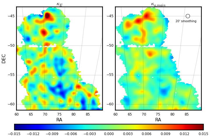
4      V. Vikram et al.
increases the signal-to-noise (S/N) of the cross-correlation between        point-spread-function (PSF) modelling, star-galaxy classification2
the lensing mass map and the foreground density map. The lensing            and photometry were done on the individual images as well as the
weight (Eqn. 10) depends on the comoving distance to the source             co-add images using software packages SE XTRACTOR (Bertin &
and lens, and the distance between them. To generate the weighted           Arnouts 1996) and PSFE X (Bertin 2011). The full SVA1 Gold
galaxy density map, we first generate a three-dimensional grid of           dataset consists of 254.4 deg2 with griz-band coverage, and 223.6
the galaxies. We estimate the density contrast in each of these cells       deg2 for Y band. The main science goal for this work is to recon-
as follows:                                                                 struct wide-field mass maps; as a result, we use the largest contin-
                            i jk  ni jk − n̄k                               uous region in the SV data: 139 deg2 in the SPT-E field.
                          δg =                                   (14)            The SVA1 Gold Catalog is augmented by: a photometric red-
                                       n̄k
                                                                            shift catalog, two galaxy shape catalogs, and an LRG catalog.
where (i, j) is the pixel index in the projected 2D sky and k is the        These catalogs are described below.
pixel index in the redshift direction. ni jk is the number of galaxies
in the i jkth cell and n̄k is the average number of galaxies per pixel in
the kth redshift bin. This three dimensional grid of galaxy density         3.1.1   Photometric redshift catalog
fluctuations will be used to estimate κg according to the discrete
version of Eqn. 8,                                                          In this work we use the photometric redshift (photo-z) estimated
                                                                            with the Bayesian Photometric Redshifts (BPZ) code (Benı́tez
               ij    3H02 Ωm     δk3D dk       (dl − dk )gl                 2000; Coe et al. 2006). The photo-z’s are used to select the main
              κg =           ∑ ∆           ∑                ,       (15)
                       2c2   k      ak     l>k      dl                      foreground and background sample (see §3.2). The details and ca-
                                                                            pabilities of BPZ on early DES data were already presented in
         ij
where κg is the weighted foreground map at the pixel (i, j); k and l        Sánchez et al. (2014), where it showed good performance among
represent indices along the redshift direction for lens and source, ∆       template-based codes. The primary set of templates used contains
is the physical size of the redshift bin, dl is the angular diameter dis-   the Coleman, Wu & Weedman (1980) templates, two starburst tem-
tance to source, gk is the probability density of the source redshift       plates from Kinney et al. (1996) and two younger starburst sim-
distribution at redshift l and δk3D is the foreground density fluctua-      ple stellar population templates from Bruzual & Charlot (2003),
tion at angular diameter distance dk . In this work, we adopt the fol-      added to BPZ in Coe et al. (2006). We calibrate the Bayesian prior
lowing cosmological parameters: Ωm = 0.3, ΩΛ = 0.7, Ωk = 0.0,               by fitting the empirical function Π(z,t|m0 ) proposed in Benı́tez
h = 0.72 (Hinshaw et al. 2013). Our results depend very weakly on           (2000), using a spectroscopic sample matched to DES galaxies and
the exact values of these cosmological parameters.                          weighted to mimic the photometric properties of the DES SV sam-
                                                                            ple used in this work. As tested in Sánchez et al. (2014), the bias
                                                                            in the photo-z estimate is ∼0.02, with 68% scatter σ68 ∼ 0.1 and
                                                                            the 3σ outlier fraction ∼2%. For this work, we use zmean , the mean
3     DATA AND SIMULATIONS
                                                                            of the Probability Distribution Function (PDF) output from BPZ as
The measurements in this paper are based on 139 deg2 of data in the         a single-point estimate of the photo-z to separate our galaxies into
SPT-E field, observed as part of the Science Verification (SV) data         the foreground and background samples. Other photo-z codes used
from DES. The SV data were taken during the period of November              in DES have been run on the same data. For this work we have also
2012 – February 2013 before the official start of the science sur-          checked our main results in §5 using an independent Neural Net-
vey. The data were taken shortly after DECam commissioning and              work code (Skynet; Bonnett 2013; Graff & Feroz 2013). We found
were used to test survey operations and assess data quality. Five           that BPZ and Skynet gives consistent results (within 1σ ) in terms
optical filters (grizY ) were used throughout the survey, with typical      of the cross-correlation between the weak lensing mass maps and
exposure times being 90 sec for griz and 45 sec for Y . The final           the foreground galaxy map.
median depth estimates of this data set in our region of interest are
g ∼ 24.0, r ∼ 23.9, i ∼ 23.0 and z ∼ 22.3.
      Below we introduce in §3.1 the relevant data used in this work        3.1.2   Shape catalogs
and in §3.3 the simulations we use to interpret our measurements.
Then we define in §3.2 two subsamples of the SV data that we                Based on the SVA1 data, two shear catalogs were produced and
identify as “foreground (lens)” and “background (source)” galaxies          tested extensively in Jarvis et al. (in preparation): the ngmix3 (ver-
for the main analysis of the paper.                                         sion 011) catalog and the im3shape4 (version 9) catalog. The main
                                                                            results shown in our paper are based on the ngmix catalog, but we
                                                                            also cross-check with the im3shape catalog to confirm that the re-
3.1    The DES SVA1 Gold galaxy catalogs                                    sults are statistically consistent.
                                                                                  The PSF model for both methods are based on the single-
All galaxies used for foreground catalogs and lensing measure-              exposure PSF models from PSFE X. PSFE X models the PSF as
ments are drawn from the DES SVA1 Gold Catalog (Rykoff et al.,              a linear combination of small images sampled on an ad hoc pixel
in preparation) and several extensions to it. The main catalog is
a product of the DES Data Management (DESDM) pipeline ver-
sion “SVA1” (Yanny et al., in preparation). The DESDM pipeline,             2 We adopt the “MODEST CLASS” classifier, which is a new classifier used
as described in Ngeow et al. (2006); Sevilla et al. (2011); Desai
                                                                            for SVA1 Gold that has been developed empirically and tested on DES
et al. (2012); Mohr et al. (2012), begins with initial image process-       imaging of COSMOS fields with Hubble Space Telescope ACS imaging.
ing on single-exposure images and astrometry measurements from              3 The open source code can be downloaded at: https://github.com/
the software package SCAMP (Bertin 2006). The single-exposure               esheldon/ngmix
images were then stacked to produce co-add images using the soft-           4 The open source code can be downloaded at: https://bitbucket.

ware package SWARP (Bertin et al. 2002). Basic object detection,            org/joezuntz/im3shape/

                                                                                                               c 0000 RAS, MNRAS 000, 000–000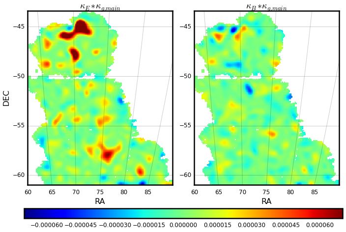
Wide Field Lensing Mass Maps from DES                         5

               Table 1. Catalogs and cuts used to construct the foreground and background sample for this work, and the number of galaxies
               in each sample after all the cuts are applied. All catalogs are based on the DES SVA1 dataset.
                                                               Background             Foreground main        Foreground LRG

                         Input catalog                  ngmix011       im3shape          SVA1 Gold              Redmagic

                         Photometric redshift                 0.6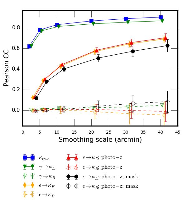
6      V. Vikram et al.
                                                                              with 1,111,487 galaxies (2.22/arcmin2 ) for ngmix and 1,013,317
                                                                              galaxies (2.03/arcmin2 ) for im3shape.
                                                                                    The foreground sample in this work serves as the tracer of
                                                                              mass. Thus it is important to construct a magnitude-limited sam-
                                                                              ple for which the number density is affected as little as possible by
                                                                              external factors. The main physical factors that contribute to varia-
                                                                              tion in the galaxy number density are the spatial variation in depth
                                                                              and seeing. Both effects can introduce spatial variation in the fore-
                                                                              ground galaxy number density, which can be wrongly identified as
                                                                              foreground mass fluctuations. We test both effects in Appendix A.
                                                                              Two subsamples are used in this work as foreground samples: the
                                                                              “main” foreground sample and the LRG foreground sample. While
                                                                              the space density of LRGs is significantly lower than that of the
                                                                              main sample, they are better tracers of galaxy clusters and groups,
                                                                              so we use them to check our results. The main foreground sample
                                                                              includes all the galaxies with i < 22 and the LRG sample includes
                                                                              the LRGs in the Redmagic LRG catalog with i < 22. This magni-
                                                                              tude selection is based on tests described in Appendix A1 to en-
                                                                              sure that our sample is shallower than the limiting magnitude for
                                                                              all regions of sky under study. The final main foreground sample
                                                                              contains 1,106,189 galaxies (2.21/arcmin2 ), while the LRG sam-
                                                                              ple contains 28,033 galaxies (0.05/arcmin2 ). Table 1 summarizes
                                                                              all the selection criteria and cuts applied on the three main samples
                                                                              used in this work.
                                                                                    Figure 1 shows the distributions of the single-point photo-z
                                                                              estimates (zmean ) for the final foreground and background samples
                                                                              (top panel), the n(z) (from the BPZ code) for the background and
                                                                              main foreground sample (second panel), and the lensing efficiency
                                                                              corresponding to the background sample (bottom panel). Note that
                                                                              the background galaxy number density is lower than expected for
                                                                              other weak lensing applications as we have made stringent redshift
                                                                              cuts to avoid overlap between the foreground and background sam-
                                                                              ples.

                                                                              3.3   Mock catalogs from simulations
                                                                              To validate the mass reconstruction procedure we use a set of sim-
                                                                              ulated galaxy catalogs “Aardvark v1.0c” developed for the DES
                                                                              collaboration (Busha et al. 2013). The full catalog covers 1/4 of the
                                                                              sky and is complete to the final expected DES depth.
                                                                                    The heart of the galaxy catalog generation is the algorithm
                                                                              Adding Density Determined Galaxies to Lightcone Simulations
                                                                              (ADDGALS; Busha et al. 2013), which aims at generating a galaxy
                                                                              catalog that matches the luminosities, colors, and clustering prop-
Figure 1. Distributions of the single-point photo-z estimates for the back-   erties of the observed data. The simulated galaxy catalog is based
ground and foreground samples used in this paper are shown in the top
                                                                              on three flat ΛCDM dark matter-only N-body simulations, one
panel. The background and the foreground main sample uses the mean of
                                                                              each of a 1050 Mpc/h, 2600 Mpc/h and 4000 Mpc/h boxes with
the PDF from BPZ for single-point estimates, while the LRG redshift esti-
mate comes independently from Redmagic (see §3.1.3). The second panel         14003 , 20483 and 20483 particles respectively. These boxes were
shows the corresponding n(z) of the background and foreground main sam-       run with LGadget-2 (Springel 2005) with 2LPTic initial condi-
ple given by BPZ. These come from the sum of the PDF for all galaxies         tions from Crocce, Pueblas & Scoccimarro (2006) and CAMB (Lewis
in the samples. The lensing efficiency (Equation 10) corresponding to the     & Bridle 2002). From an input luminosity function, galaxies are
background sample is shown in the third panel.                                drawn and then assigned to a position in the dark matter simula-
                                                                              tion volume according to a statistical prescription of the relation
                                                                              between the galaxy’s magnitude, redshift and local dark matter den-
                                                                              sity. The prescription is derived from a high-resolution simulation
sample only serves as a “backlight” for the foreground structure we           using SubHalo Abundance Matching techniques (Conroy, Wech-
are interested in, it need not be complete. Therefore the most im-            sler & Kravtsov 2006; Reddick et al. 2013; Busha et al. 2013).
portant selection criteria for the background sample is to use galax-         Next, photometric properties are assigned to each galaxy, where
ies with accurate shear measurements. Our source selection criteria           the magnitude-color-redshift distribution is designed to reproduce
are based on extensive tests of shear catalog as described in Jarvis          the observed distribution of SDSS DR8 and DEEP2 data. The size
et al. (in preparation). After applying the conservative selection of         distribution of the galaxies is magnitude-dependent and modelled
background galaxies and our background redshift cut we are left               from a set of deep (i ∼26) SuprimeCam i-band images, which were

                                                                                                                c 0000 RAS, MNRAS 000, 000–000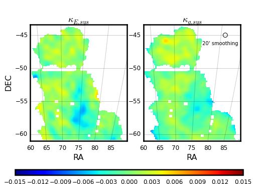
Wide Field Lensing Mass Maps from DES                         7
taken at with seeing conditions of 0.6”. Finally, the weak lens-         DES data. We compare optically identified groups and clusters of
ing parameters (κ and γ) in the simulations are based on the ray-        galaxies in our data based on Redmapper with the reconstructed
tracing algorithm Curved-sky grAvitational Lensing for Cosmolog-         mass map. We overlay in Figure 4 Redmapper clusters and groups
ical Light conE simulatioNS (CALCLENS; Becker 2013). The ray-            on the mass map as black circles. The size of these circles corre-
tracing resolution is accurate to ' 6.4 arcseconds, sufficient for the   sponds to the optical richness of these structures. Also, only objects
usage in this work.                                                      with optical richness λ greater than 20 and redshift between 0.1
      Aside from the intrinsic uncertainties in the modelling in the     and 0.5 are shown in the figure. According to Rykoff et al. (2012)
mock galaxy catalog (related to the input parameters and uncer-          and Saro et al. (in preparation), this corresponds to cluster masses
tainty in the galaxy-halo connection), there are also many real-         larger than a few times 1014 M . It is evident from this figure that
world effects that are not included in these simulations, including      the structures in the weak lensing mass map have significant corre-
as depth variation, seeing variation and shear measurement uncer-        lation with the distribution of optically identified Redmapper clus-
tainties. As a result, we use the simulations primarily as a tool to     ters.
understand the impact of various effects on the expected signal, and           From the mass and galaxy maps in Figure 2 and Figure 4
a sanity check to confirm that our measurement method is produc-         we identified large peaks at the positions (RA, DEC) = (71.0, -
ing reasonable results.                                                  45.0), (70.0, -47.8), (69.8, -54.5) and (69.1, -57.3), and large voids
                                                                         at (RA, DEC) = (65.7, -49.0), (74.8, -54.8), (75.7, -58.0), (82.8,
                                                                         -59.5). Analyzing the redshift distribution of the foreground struc-
4     RESULTS: MASS MAPS AND GALAXY CLUSTERS                             ture at these locations shows that the peaks indeed correspond to
                                                                         supercluster like structures that are typically localized in the red-
In Figure 2 we show our final convergence maps generated using           shift range 0.3 − 0.4, though in at least one case there is evidence
the data described in §3.1 and the methods described in §2.2 and         for multiple structures at different redshifts. The tight photo-z ac-
§2.3. For the purpose of visualization we present maps for 20 ar-        curacy of the Redmapper clusters (σz ≈ 0.01(1 + z)) gives us some
cmin Gaussian smoothing. In the top left panel we show the E-            confidence in the identification of real 3D structures. The trans-
mode convergence map generated from shear. The top right panel           verse spatial extent of the superclusters is typically greater than 10
shows the weighted foreground galaxy map from the main sample,           Mpc. We believe this approach provides a powerful tool for iden-
κg,main map. In both of these panels, red areas correspond to over-      tifying superstructures in the Universe which would otherwise be
densities and blue areas correspond to under densities. The bottom       hard to spot. The size and mass of the superclusters are of interest
left and bottom right panels show the product of the κE (left) and       for cosmology as they represent the most massive end of the mat-
κB (right) maps with the κg,main . Visually we see that there are more   ter distribution. We defer more detailed studies of the superclusters
positive (correlated) areas for the κE map compared to the κB map,       and voids to follow up work.
indicating clear detection of the weak lensing signal in these maps.
Note that these positive regions could be either mass over-densities
or under-densities. In §5, we present a quantitative analysis of this
                                                                         5     RESULTS: MASS MAPS AND CORRELATION WITH
correlation.
                                                                               GALAXY DISTRIBUTION
                                                                         In this section we quantitatively analyze the extent to which mass
4.1    Noise estimates for the mass maps
                                                                         follows galaxy density in the data. To do this, we cross-correlate
To estimate the significance of the structures in the mass maps, it is   the weak lensing mass map with the weighted foreground galaxy
important to understand the noise properties of these maps. Uncer-       density map. The correlation is quantified via the Pearson cross-
tainties in the lensing convergence map include contributions from       correlation coefficient as described in §5.1. We cross check the re-
both shape noise and measurement uncertainties, which is affected        sults using simulations in §5.2.
by the number density of galaxies across the field and the shear
measurement method.
      We estimate the uncertainties on each pixel by randomising         5.1    Quantifying the galaxy-mass correlation
the shear measurements on each galaxy. A thousand random back-           We smooth both the convergence maps generated from weak lens-
ground galaxy catalogs were generated by shuffling the shear val-        ing and from the foreground galaxy density with a Gaussian filter.
ues between all the galaxies. We then construct κE and κB maps           These smoothed maps are used to estimate the correlation between
from these randomized catalogs in the same way as in Figure 2.           the foreground structure and the weak lensing convergence maps.
The RMS map for these 1000 random samples is used as the noise           We calculate the correlation as a function of the smoothing scale
map. Dividing the signal map (Figure 2) by the noise map gives           (i.e. the size of the Gaussian filter). The correlation is quantified
an estimate for the S/N of the different structures in the maps, as      via the Pearson correlation coefficient defined as
shown in Figure 3. These values are consistent with those predicted
                                                                                                             hκE κg i
via Equation 13 and simulations described in §5.2. The bottom pan-                                ρκE κg =            ,                   (16)
els of Figure 3 show the distribution of the S/N values for both E                                           σκE σκg
and B-mode maps for data as well as simulations. We find that the        where hκE κg i is the covariance between κE and κg ; σκE and σκg
B-mode distribution is consistent with a Gaussian distribution and       are the standard deviation of the κE map, and the κg map from
the E-mode gives more extreme values.                                    either the foreground main galaxy sample or the foreground LRG
                                                                         sample. In this calculation, pixels in the masked region are not used.
                                                                         We also remove pixels within 10 arcmin of the boundaries to avoid
4.2    Correlation with known structures
                                                                         significant artefacts from the smoothing.
In this section we compare our mass map with optically identified             Figure 5 shows the Pearson correlation coefficient as func-
clusters using Redmapper v6.3.3 (Rykoff et al. in preparation) from      tion of smoothing scales from 2 to 40 arcmin. We find that there

c 0000 RAS, MNRAS 000, 000–000
8 V. Vikram et al.
Figure 2. The upper left panel shows the E-modes of the weak lensing convergence map. The upper right shows the weighted foreground galaxy map from
the main sample, or κg,main . The lower two panels show the product maps of the E-mode (left) and B-mode (right) convergence map with the κg,main map. All
maps are generated with a 5 arcmin pixel scale and 20 arcmin Gaussian smoothing. Red areas corresponds to overdensities and blue areas to underdensities in
the upper panels. White regions correspond to the survey mask. The scale of the Gaussian smoothing
√ kernel is indicated by the circle on the upper right corner,
with a radius of 20 arcmin (the equivalent radius of a top-hat kernel is larger by a factor of 2).
c 0000 RAS, MNRAS 000, 000–000Wide Field Lensing Mass Maps from DES 9
Figure 3. The top panel shows the S/N map for the mass map in Figure 2 estimated via randomized errors described in §4.1. Note that due to the Gaussian
smoothing kernel, there is some mixing of scales which leads to higher contrasts in the cores of over and under-dense regions compared to top-hat smoothing.
The bottom panel shows the normalized S/N distributions for both maps, overlaid by those measured from simulations described in §5.2. The red dashed lines
in both bottom panels show a Gaussian fit to the B-mode S/N.
is significant correlation between the weak lensing E-mode con- of the 10 deg2 regions each time. We found that the estimated un-
vergence and convergence from different foreground samples, with certainties do not depend significantly on the exact value of patch
increasing correlation towards large smoothing scale. This trend is size. We estimate the correlation coefficient after removing one of
expected for noise-dominated maps, because the larger smoothing those patches from the sample to get jackknife realizations of the
scales reduce the noise fluctuations in the map significantly. A sim- cross-correlation coefficient ρ j . Finally, the variance is estimated
ilar trend is found when using the LRGs as foreground instead of as
the general magnitude-limited galaxy sample. The lower Pearson
N −1
correlation between the mass map and LRG sample is because of ∆ρ = (ρ j − ρ̄)2 , (17)
N ∑j
the larger shot noise due to the lower number density compared
to the magnitude-limited foreground sample. The error bar on the
where j runs over all the N jackknife realizations and ρ̄ is the aver-
correlation coefficient is estimated based on jackknife resampling.
age correlation coefficients of all patches.
We divide the observed sky into jackknife regions of size 10 deg2
We find that the Pearson correlation coefficient between κg
and recalculate the Pearson correlation coefficients, excluding one
from the main foreground galaxy sample (LRG sample) and weak
c 0000 RAS, MNRAS 000, 000–00010 V. Vikram et al.
Figure 4. The DES SV mass map along with foreground galaxy clusters detected using the Redmapper algorithm. The clusters are overlaid as black circles
with the size of the circles indicating the richness of the cluster. Only clusters with richness greater than 20 and redshift between 0.1 and 0.5 are shown in
the figure. The upper right corner shows the correspondence of the optical richness to the size of the circle in the plot. It can be seen that there is significant
correlation between the mass map and the distribution of galaxy clusters. Several superclusters and voids can be identified in the joint map.
lensing E-mode convergence is 0.39 ± 0.06 (0.36 ± 0.05) at 10 ar- 5.2 Comparison with mock catalogs
cmin smoothing and 0.52±0.08 (0.46±0.07) at 20 arcmin smooth-
ing. This corresponds to a ∼ 6.8σ (7.5σ ) significance at 10 arcmin At this point, it is important to verify whether our measurements
smoothing and ∼ 6.8σ (6.4σ ) at 20 arcmin smoothing. As a zeroth- in the data are consistent with what is expected. We investigate
order test of systematics we also estimated the correlation between this using the simulated catalogs described in §3.3. As the simu-
the B-mode weak lensing convergence and the κg maps. We find lations lack several realistic systematic effects in the data, these
that the correlation between κB and the main foreground sample tests mainly serve as a guidance for us to understand: (1) the origin
is consistent with zero at all smoothing scales. Similarly, the cor- of the B-mode in the κ maps, (2) the approximate expected level of
relation between E and B modes of κ is consistent with zero. For ρκκg under pixelization and smoothing, (3) the effect on ρκκg from
comparison, we show the same plot calculated for the im3shape photo-z uncertainties and cosmic variance, and (4) the effect on the
catalog in Figure 6. We find very similar results, with slightly larger maps and ρκκg from the survey mask.
correlation between κE and κB at the 1σ level. We construct a sample similar to the SV data. The same red-
shift, magnitude, and number density cuts in Table 1 are applied to
the simulations to form a foreground and a background sample. We
c 0000 RAS, MNRAS 000, 000–000Wide Field Lensing Mass Maps from DES 11
Figure 5. This figure shows the Pearson correlation coefficient between foreground galaxies and convergence maps as a function of smoothing scale. The solid
and open symbols show the E and B-mode correlation coefficients respectively. The black circles are for the main foreground sample and the red circles for
foreground LRGs. The grey shaded regions show the 1σ bounds for E and B mode correlations from simulations for the main foreground sample with the
same pixelization and smoothing (see §5.2 for details). We do not show the same simulation results for the LRG sample. The detection significance for the
correlation is in the range ∼ 5 − 7σ at different smoothing scales. The green points show the correlation between E and B-modes of the mass map. The various
B-mode correlations are consistent with zero. Uncertainties on all measurements are estimated based on jackknife resampling.
Figure 6. Same as Figure 5 but using the im3shape galaxy catalog.
choose to simulate the main foreground sample as the LRG fore- steps, in order of increasing similarities to data: (1) pixelating and
ground sample selection in the simulations is less controllable. For smoothing the true κ values; (2) constructing the κ values from the
the background sample, we add a random Gaussian of RMS 0.29 true γ values; (3) construct the κ values from the galaxy elliptici-
per component to the true shear in the simulations to generate a ties; (4) repeat (3) using a photo-z model for the foreground and the
model for the ellipticities that matches the data. We then create a background instead of the true redshift; (5) repeat (4) for different
κg map from the main foreground sample and a κ map from the regions on the sky; (6) repeat (5) with the SV survey mask.
background sample the same way as is done in the data. The cross- The difference between (1) and (2) measures the quality of
correlation coefficient ρκκg is calculated from these simulated maps the KS reconstruction method. The difference between (2) and (3)
as in §5. We consider the same range of smoothing scales for the shows the effect of shape noise and measurement noise. Steps (4),
maps when calculating ρκκg as that in Figure 6. (5) and (6) then show the effect of photo-z uncertainties, cosmic
The simulations provide us a controlled way of separating the variance and masking. Note that we estimate the effect of sample
different sources of effects. We construct the maps in the following variance by generating maps for 4 different regions on the sky. Also
c 0000 RAS, MNRAS 000, 000–00012 V. Vikram et al.
Figure 8. Pearson correlation coefficient ρXκg between the different sim-
ulated maps shown in Figure 7 as a function of smoothing scale. X repre-
sents the different κ maps as listed in the legend. This plot is the simulation
version of Figure 5, where one can see how the measured values in the data
could have been degraded due to various effects. The qualitative trend of the
correlation coefficients as a function of smoothing scale is consistent with
that observed in data. When reconstructing κE from the true γ small errors
are introduced due to the nonlocal reconstruction, lowering the correlation
coefficient by a few percent. Adding shape noise to the shear measurement
lowers the signal significantly, with the level of degradation dependent on
the smoothing scale. Adding photo-z uncertainties changes the signal by a
few percent. Finally, placing an SV-like survey mask changes the signal by
∼10%. The black curve with its error bars corresponds to the shaded region
in Figure 5.
for the steps (4)-(6) above, we generate each of the maps with 20
different realisations of the shape noise.
5.2.1 Maps from simulations
Figure 7 shows the various maps generated from one particular
patch of the simulations in this procedure for 5 arcmin pixels and 20
Figure 7. Maps from simulations that are designed to mimic the data in our arcmin smoothing scales (consistent with that in Figure 2). The am-
analysis. The simulations are generated for a field of size 15×17.6 deg2 with plitude of κE and κB both become larger than in the true maps when
similar redshift and magnitude cuts for the foreground and the background shape noise is added, and the resulting κE map has only slightly
sample as the data. The true κ and κg maps are shown in the first row, where higher contrast than the κB map. When photo-z uncertainties are
κg is modelled for the main foreground sample. The reconstructed κE and
included, we see that the peaks and voids in the κE maps visibly
κB maps from the true γ are shown in the first two panels of the second
row, followed by the κE and κB maps reconstructed from the ellipticity (ε)
move around. Applying the mask mainly changes the morphology
values. The last row first shows the κE and κB constructed from ε with of the structures in the maps around the edges. Comparing the last
photo-z uncertainties, then the same maps with an SV survey mask applied. κE panel in Figure 7 and Figure 2, we see that the amplitude and
The last two panels on the bottom most closely match the data. qualitative scales of the variation in the κE maps are similar. On the
other hand, if we compare the κg maps in the simulations with the
κg maps in Figure 2, we find some qualitative differences between
the simulations and the data. The simulation contains more small
scale structure and low-κg regions compared to the data. We do not
investigate this issue further here, as the level of agreement in the
simulations and the data is sufficient for our purpose.
c 0000 RAS, MNRAS 000, 000–000Wide Field Lensing Mass Maps from DES 13
5.2.2 Correlation coefficients from simulations Table 2. Quantities examined in our systematics tests.
Figure 8 shows the mean Pearson correlation coefficient between Map name description
the different maps as a function of smoothing scales for the 80 sets
kE (signal) κE from γ1 , γ2 for background sample
of simulated maps (4 different areas in the sky and 20 realisations
kg (signal) κg from main foreground sample
of shape noise each). The error bars indicate the RMS spread of
kB κB from γ1 , γ2 for background sample
these 80 simulations. ns star number per pixel
We find that ρκtrue κg is 10-20% below 1, which is the case for ng b galaxy number per pixel for background sample
perfect correlation. Several factors contribute to this. First, the fore- snr signal-to-noise of galaxies in im3shape
ground galaxy sample only includes a finite redshift range, and not mask fraction of area masked in galaxy postage stamp
all galaxies that contribute to the κtrue map. Second, the presence g1 average γ1 for background sample
of a redshift-dependent galaxy bias adds further complication to g2 average γ2 for background sample
the correlation coefficient. The effect of converting from the true psf e1 average PSF ellipticity
shear γ to convergence lowers the correlation coefficient by about psf e2 average PSF ellipticity
psf T average PSF size
3%. This is a measure of the error in the KS conversion under fi-
psf kE κE generated from average PSF ellipticity
nite area and resolution of the shear fields. The main degradation
psf kB κB generated from average PSF ellipticity
of the signal comes when shape noise and measurement noise is in- zp b mean photo-z for background sample
cluded. Photo-z uncertainties in both the foreground and the back- zp f mean photo-z for foreground sample
ground sample changes the correlation coefficient slightly. Finally, ebv mean extinction
the survey mask lowers the signal by ∼ 10%. skysigma RMS sky brightness in ADU
The final correlation coefficient after considering all the ef- sky mean sky brightness in ADU
fects discussed above is shown by the black curve in Figure 8 and maglim mean limiting i-band AB magnitude
overplotted as the shaded region in Figure 5. We find that the de- exptime mean exposure time in seconds
pendence of ρκκg on the smoothing scale in the simulation is qual- airmass mean airmass
itatively and quantitatively very similar to that seen in Figure 5.
on the following simple diagnostic quantity:
ρ̂κE Θ ρ̂κg Θ
ρ̂κE κg ;Θ = (18)
6 SYSTEMATIC EFFECTS ρ̂ΘΘ
In §4.1 we evaluated the statistical uncertainties on the mass map with ρ̂XY being the cross-correlation function, which is effectively
and the correlation between the mass map and the foreground the unnormalized Pearson correlation coefficient between X and Y ,
galaxy density maps. In this section we examine the possible sys- or
tematic uncertainties in our measurement. We focus on the cross ρ̂XY = hXY i. (19)
correlation between our weak lensing mass map κE and the main
foreground density map κg,main . To simplify the notation, we omit Equation 18 measures the contribution from some systematics field
the “main” in the subscript and use κg to represent the main fore- Θ to ρ̂κE κg . We calculate ρ̂κE κg ;Θ with Θ being any of the 20 quan-
ground map in this section. tities in Table 2 (excluding the signal). Figure 9 shows the normal-
We investigate the potential contamination from systematic ef- ized cross-correlation coefficient ρ̂κE κg ;Θ /ρ̂κE κg values for all the
fects on the cross-correlation coefficient ρκE κg . That is, we consider quantities considered for 10 and 20 arcmin smoothing, with the red
the situation where part of the correlation between the mass map dashed line at 5%. The error bars are estimated by jackknife re-
and the κg map is not cosmological, but rather caused by other sampling similar to that described in §5.1, and the two panels show
physical systematic effects that are correlated with both maps si- the results for ngmix and im3shape respectively. The normalized
multaneously. We examine these systematic uncertainties in our cross-correlation coefficient is a measure of the fractional contam-
measurement by looking at the spatial correlation of various quan- ination in the Pearson coefficient (Equation 16) from each of the
tities with the κE map and the κg map. systematics maps Θ.
As discussed in Appendix A, there are several factors that can We find that for ngmix all quantities show contributions to the
contaminate the δg maps. For example, depth and PSF variations systematic uncertainties at 10 arcmin smoothing to be at the level
in the observed field can introduce artificial clustering in the fore- of 5% or lower, while the systematics increase to up to 15% when
ground galaxy density map. Although we use magnitude and red- smoothing at the 20 arcmin scale (though with large error bars on
shift cuts according to the tests in Appendix A, one can expect some the systematics estimation). For im3shape, most of the values stay
level of residual effects on the κg maps. The κE map is constructed below 5% for both smoothing scales. The largest contribution in
from shear catalogs of the background sample, thus systematics in both cases come from the variation in the PSF properties (psf e1,
the shear measurement will propagate into the κE map. In Jarvis et psf e2, psf kB). Since all these PSF quantities are correlated with
al. (in preparation), extensive tests of systematics have been carried each other, and many other parameters (g1, g2, snr, maglim) are
out on the shear catalog. Therefore here we focus on the systematics correlated with the PSF properties, we do not expect the total sys-
that are specifically relevant for mass mapping and the correlation tematics contamination to be a direct sum of all these parameters.
coefficient Eqn. 16. Instead, we discuss in Appendix B how one can isolate the inde-
We identify several possible sources of systematics for the pendent contributions of the systematics via a Principal Component
background and foreground sample as listed in Table 2. We gen- Analysis approach and correct for them. We find that the correction
erate maps of these quantities that are pixelated and smoothed on changes the final Pearson correlation coefficient by 3.5% relative to
the same scale as the κE and κg maps. We then evaluate the contri- the original ρκE κg measured in §5.
bution of these effects to the correlation coefficient (Eqn. 16) based Finally, to check the level of systematic contamination in our
c 0000 RAS, MNRAS 000, 000–00014 V. Vikram et al.
Figure 9. The normalised cross-correlation coefficient ρ̂κE κg ;Θ is shown for 20 different systematic uncertainty parameters. The systematics parameters,
represented by Θ, are listed in Table 2 and shown for two smoothing scales. The ρ̂κE κg ;Θ values are normalized by ρ̂κE κg to show the relative magnitude of the
systematic and the signal. The red dashed line indicates where the systematic is 5% of ρ̂κE κg . The error bars are estimated from resampling the foreground and
background galaxy sample in patches of size 10 deg2 . The left panel is calculated for ngmix while the right panel is for im3shape.
Figure 10. Pearson correlation coefficient ρκE Θ where Θ represents the quantities listed in Table 2. We show the statistics for two smoothing scales and for
both ngmix (left) and im3shape (right). The right-most points in both panel correspond to the detection signal in Figure 5 and Figure 6. The error bars are
estimated from resampling the foreground and background galaxy sample in patches of size 10 deg2 . Note that this is a different statistic from that in Figure 9,
thus the y-axis values are not directly comparable.
κE map itself, we also calculate the Pearson correlation coefficient be intrinsically non-zero, even if there were no systematics contam-
(Eqn. 16) between the various maps in Table 2 and our κE map. ination in the maps.
Note that this contamination may or may not be pronounced in Fig-
ure 9 since the statistics plotted there also take into account the cor-
relation of κg with the various quantities. This test is independent 7 CONCLUSIONS
of the foreground map, therefore is important for applications of the
κE map that do not also use the foreground maps. Figure 10 shows Weak lensing mass maps, or convergence maps, enable a number of
the resulting 21 Pearson correlation coefficients. We find that the cosmological studies: cross-correlations with galaxies, clusters and
signal shown in the right-most points in the plot (ρκE κg ) is larger filaments, and with Sunyaev-Zel’dovich (SZ) or lensing maps from
than all other correlations by at least a factor of ∼3. the cosmic microwave background (CMB). In addition, 2-point cor-
relation functions of the convergence field provide a useful and sim-
ple check on the measurements made directly with the shear, while
We also note that in both of these tests, the area of the map is higher order correlations are easier to measure and interpret than
not big enough to ignore the fact that some of these correlations can those of the two-component shear field.
c 0000 RAS, MNRAS 000, 000–000Wide Field Lensing Mass Maps from DES 15
In this work, we present a weak lensing mass map based ‘Origin and Structure of the Universe’. FS acknowledges financial
on galaxy shape measurements in the 139 deg2 SPT-E field from support provided by CAPES under contract No. 3171-13-2
the Dark Energy Survey Science Verification data. We have cross- Funding for the DES Projects has been provided by the U.S.
correlated the mass map with maps of galaxy and cluster samples Department of Energy, the U.S. National Science Foundation, the
in the same dataset. Ministry of Science and Education of Spain, the Science and Tech-
We constructed mass maps from the foreground Redmagic nology Facilities Council of the United Kingdom, the Higher Ed-
LRG and general magnitude-limited galaxy samples under the as- ucation Funding Council for England, the National Center for Su-
sumption that mass traces light. We find that the E-mode of the percomputing Applications at the University of Illinois at Urbana-
convergence map correlates with the galaxy based maps with high Champaign, the Kavli Institute of Cosmological Physics at the Uni-
statistical significance. We repeated this analysis at various levels of versity of Chicago, the Center for Cosmology and Astro-Particle
smoothing scales and compared the results to measurements from Physics at the Ohio State University, the Mitchell Institute for Fun-
mock catalogs that reproduce the galaxy distribution and lensing damental Physics and Astronomy at Texas A&M University, Fi-
shape noise properties of the data. The Pearson cross-correlation nanciadora de Estudos e Projetos, Fundação Carlos Chagas Filho
coefficient is 0.39 ± 0.06 (0.36 ± 0.05) at 10 arcmin smoothing de Amparo à Pesquisa do Estado do Rio de Janeiro, Conselho Na-
and 0.52 ± 0.08 (0.46 ± 0.07) at 20 arcmin smoothing for the main cional de Desenvolvimento Cientı́fico e Tecnológico and the Min-
(LRG) foreground sample. This corresponds to a ∼ 6.8σ (7.5σ ) istério da Ciência e Tecnologia, the Deutsche Forschungsgemein-
significance at 10 arcmin smoothing and ∼ 6.8σ (6.4σ ) at 20 ar- schaft and the Collaborating Institutions in the Dark Energy Survey.
cmin smoothing. We get comparable values from the mock cata- The DES data management system is supported by the Na-
logs, indicating that statistical uncertainties, not systematics, dom- tional Science Foundation under Grant Number AST-1138766.
inate the noise in the data. The B-mode of the mass map is consis- The DES participants from Spanish institutions are partially sup-
tent with noise and its correlations with the foreground maps are ported by MINECO under grants AYA2012-39559, ESP2013-
consistent with zero at the 1σ level. 48274, FPA2013-47986, and Centro de Excelencia Severo Ochoa
To examine potential systematic uncertainties in the conver- SEV-2012-0234, some of which include ERDF funds from the Eu-
gence map we identified 20 possible systematic tracers such as see- ropean Union.
ing, depth, PSF ellipticity and photo-z uncertainties. We show that The Collaborating Institutions are Argonne National Labora-
the systematics effects are consistent with zero at the 1 or 2σ level. tory, the University of California at Santa Cruz, the University of
In Appendix B, we present a simple scheme for the estimation of Cambridge, Centro de Investigaciones Energeticas, Medioambien-
systematic uncertainties using Principal Component Analysis. We tales y Tecnologicas-Madrid, the University of Chicago, University
discuss how these contributions can be subtracted from the mass College London, the DES-Brazil Consortium, the Eidgenössische
maps if they are found to be significant. Technische Hochschule (ETH) Zürich, Fermi National Accelera-
The results from this work open several new directions of tor Laboratory5 , the University of Edinburgh, the University of
study. Potential areas include the study of the relative distribution Illinois at Urbana-Champaign, the Institut de Ciencies de l’Espai
of hot gas with respect to the total mass based on X-ray or SZ ob- (IEEC/CSIC), the Institut de Fisica d’Altes Energies, Lawrence
servations, estimation of galaxy bias, constraining cosmology using Berkeley National Laboratory, the Ludwig-Maximilians Univer-
peak statistics, and finding filaments in the cosmic web. The tools sität and the associated Excellence Cluster Universe, the Univer-
that we have developed in this paper are useful both for identifying sity of Michigan, the National Optical Astronomy Observatory, the
potential systematic errors and for cosmological applications. The University of Nottingham, The Ohio State University, the Univer-
observing seasons for the first two years of DES are now complete sity of Pennsylvania, the University of Portsmouth, SLAC National
(Diehl et al. 2014) and contain an area well over ten times that of Accelerator Laboratory, Stanford University, the University of Sus-
the SV data, though shallower by about half a magnitude. The full sex, and Texas A&M University.
DES survey area will be ∼ 35 times larger than that presented here, This paper has gone through internal review by the DES col-
at roughly the same depth. The techniques and tools developed in laboration.
this work will be applied to this new survey data, allowing signifi-
cant expansion of the work here.
REFERENCES
ACKNOWLEDGEMENTS Amara A. et al., 2012, MNRAS, 424, 553
Bacon D. J., Massey R. J., Refregier A. R., Ellis R. S., 2003, MN-
We are grateful for the extraordinary contributions of our CTIO col-
RAS, 344, 673
leagues and the DECam Construction, Commissioning and Science
Bacon D. J., Refregier A. R., Ellis R. S., 2000, MNRAS, 318, 625
Verification teams in achieving the excellent instrument and tele-
Bahcall N. A., Fan X., 1998, ApJ, 504, 1
scope conditions that have made this work possible. The success of
Bartelmann M., Narayan R., Seitz S., Schneider P., 1996, ApJ,
this project also relies critically on the expertise and dedication of
464, L115
the DES Data Management group.
Bartelmann M., Schneider P., 2001, Physics Reports, 340, 291
We thank Jake VanderPlas, Andy Connolly, Phil Marshall, and
Becker M. R., 2013, MNRAS, 435, 115
Rafal Szepietowski for discussions and collaborative work on mass
Benı́tez N., 2000, ApJ, 536, 571
mapping methodology. CC and AA are supported by the Swiss
Bergé J., Amara A., Réfrégier A., 2010, ApJ, 712, 992
National Science Foundation grants 200021-149442 and 200021-
143906. SLB and JZ acknowledge support from a European Re-
search Council Starting Grant with number 240672. DG was sup-
ported by SFB-Transregio 33 ‘The Dark Universe’ by the Deutsche 5Operated by Fermi Research Alliance, LLC under Contract No. De-
Forschungsgemeinschaft (DFG) and the DFG cluster of excellence AC02-07CH11359 with the United States Department of Energy.
c 0000 RAS, MNRAS 000, 000–000You can also read