Implementation of a Bespoke, Collaborative-Filtering, Matrix-Factoring Recommender System Based on a Bernoulli Distribution Model for Webel

Implementation of a Bespoke,
Collaborative-Filtering, Matrix-Factoring
 Recommender System Based on a
 Bernoulli Distribution Model for Webel

 Martín Bosco Domingo Benito
 4° Curso - Grado de Ingeniería del Software (Plan 2014)

 Mayo 2021

 Tutor: Raúl Lara Cabrera

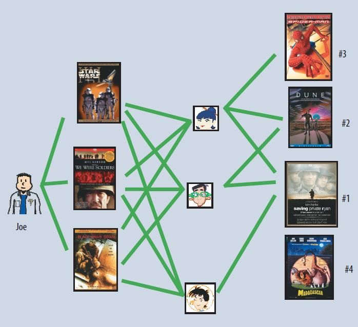
Table of Contents
Abstract .................................................................................................................................................. 2
Resumen ................................................................................................................................................. 3
Objectives ............................................................................................................................................... 4
Introduction to Recommender Systems ............................................................................................... 5
 Information within a Recommender System .................................................................................... 6
 Types of Recommender Systems ...................................................................................................... 6
 Demographic Filtering ................................................................................................................... 7
 Content-Based Filtering ................................................................................................................. 7
 Collaborative Filtering ................................................................................................................... 8
 Evaluating Recommender Systems ................................................................................................. 14
 Evaluation based on well-defined metrics .................................................................................. 14
 Evaluation based on beyond-accuracy metrics........................................................................... 17
 Overview & State of the Art .............................................................................................................. 18
A Closer Look to Matrix Factorisation (MF).......................................................................................... 21
The BeMF Model ................................................................................................................................... 25
Procedure ............................................................................................................................................. 27
 Tool installation and environment setup........................................................................................ 28
 Practical work................................................................................................................................... 28
 Synthetic data generation (Data augmentation) ........................................................................ 30
 Instruction and integration.............................................................................................................. 32
Environmental & Social Impacts ......................................................................................................... 34
Ethical and Professional Responsibility .............................................................................................. 36
Conclusions and proposed work ......................................................................................................... 37
Bibliography ......................................................................................................................................... 38
Annex I: Acronyms & Abbreviations ..................................................................................................... 41

 1

Abstract
This project documents the process of building and training a Collaborative-Filtering, Matrix-
Factoring Recommender System based on the proposed BeMF model in [1] and adapted for Webel,
a software company aiming to provide at-home services offered by professionals through a mobile
app. It also includes the successful preparation and employee training for future integration with
their existing systems and subsequent launch into production.

 2

Resumen
Este proyecto documenta el proceso de construcción y entrenamiento de un Sistema de
Recomendación por Filtrado Colaborativo y Factorización Matricial basado en el modelo BeMF
propuesto en [1] adaptado para Webel, una empresa software dirigida a ofrecer servicios a
domicilio ofertados por profesionales a través de una aplicación móvil. Se incluye la preparación
del entorno y empleados para la futura integración con sus sistemas existentes y subsecuente
lanzamiento a producción.

 3

Objectives
 1. To introduce the reader to the technical background required to understand
 Recommender Systems and the BeMF model in particular.
 2. To delineate and elicit customer’s needs and desires, as well as the acceptance criteria
 and evaluation methods and metrics.
 3. To design the plan for a Recommendation System based on existing research (BeMF
 model) to fit the customer’s needs.
 4. To successfully implement and train the aforementioned model with the provided data.
 5. To instruct the client on how to improve, train and integrate the model into the existing
 systems for future use in a real-world environment.

 4

Introduction to Recommender Systems
A Recommender System or Recommendation System (which will be referred to as RS from now
onwards) is, according to Wikipedia: “a subclass of information filtering systems that seeks to
predict the ‘rating’ or ‘preference’ a user would give to an item” [2]; and in the blog Towards Data
Science, they are defined as “algorithms aimed at suggesting relevant items to users.” [3]

RSs are ubiquitous all over the internet and are one of the main vehicles of customer satisfaction
and retention for many companies offering e-commerce and/or entertainment products like
Amazon, YouTube, TikTok, Instagram or Netflix [4].

The basis for all RSs are the following 3 main pillars [5]:
 ● Users: The target of the recommendations.
 ● Items: The products or services to be recommended. The system will extract the
 fundamental features of each item to recommend it to interested users.
 ● Ratings: The quantification of a particular user’s interest for a specific item. This voting can
 be implicit (the user expresses their interest on a pre-established scale) or explicit, (the
 system infers the preference based upon the user-item interaction).
These 3 pillars come to form the User-Item matrix, as seen in Figure 1.

 Figure 1. Illustration of a User-Item (Ratings) matrix [3].

Knowing what a user would like to see is crucial to keep them on a site, and so is predicting their
next need or desire to get them to buy a specific product or service, by catering to each
individual’s specific interests. For this to work, a vast amount of data is required in order to
establish certain profiles and be able to link individuals to items they may be potentially
interested in. In the case of Netflix, as well as many others, “customers have proven willing to
indicate their level of satisfaction [...], so a huge volume of data is available about which movies
appeal to which customers” [4]. And thus, it can be concluded that said aspect is oftentimes not
the major bottleneck for large corporations, although it most certainly can be for small and
medium-sized enterprises or SMEs, as will be seen later on.

 5

How the aforementioned linkage between a user and its recommendation is established relies on
the type of RS implemented.

Information within a Recommender System
There are 4 main levels of information upon which an RS can work, from lowest to highest amount
and complexity of information used [5]:
 1. Memory-based level: Encompasses the ratings (whether implicit or explicit).
 2. Content-based level: Adds additional information to improve the quality of the
 recommendations, such as users’ demographic info (age, occupation, ethnicity…), app-
 related activity, or items’ implicit and explicit information (e.g., how many times is an item
 looked at - implicit, what actors star in a movie - explicit).
 3. Social-information-based level: Employs data pertaining to the social web the user is part
 of (what items are recommended to friends, who are the user’s followers and who does the
 user follow...). Items are tagged by users and are classified based on user interactions with
 them, such as likes, dislikes, shares, etc.
 4. Context-based level: Makes use of the Internet of Things (IoT) to incorporate implicit
 personal information of the user through other devices regarding personal habits,
 geolocation, biometrics… Items-wise, environmental integration, geolocation and many
 others are examples of data used for recommendation. The results are recommendations
 akin to “We noticed you’re sweating and going for a walk, John. These are the best ice-cream
 restaurants around you to enjoy a cool break on this hot summer day”.

Types of Recommender Systems
There are several types of RSs, and the main difference stems from the way they filter information,
which births three main paradigms: Demographic Filtering, Content-based Filtering and
Collaborative Filtering. Figure 2 showcases a breakdown in their individual branches:

 Figure 2. Overview of the different recommender system algorithms (sans demographic filtering) [3].

 6

Demographic Filtering
“Recommendations are given based upon the demographic characteristics of users, founded on
the assumption that users with similar characteristics will have similar interests. These types of
recommendations are often dull, inaccurate and rarely innovative.” [5]

This type of filtering results in extremely biased RSs in the vast majority of cases, a tendency the
ML field is trying to move away from, therefore rendering it a filtering method which has fallen out
of favour and is seldom used. Added to its frequently useless recommendations, it is shadowed by
the other two alternatives (hence why it is not included in the above graphic and will fall outside of
the scope of this project).

Content-Based Filtering
Content-based Filtering relies on creating a profile around a user’s or an item’s
characteristics/information/interest, which, in the case of users, tend to be of personal or sensitive
nature, such as age, gender, salary, religion… [4].

The idea of Content-based methods is to try to build a model, based on the available “features”,
that explains the observed user-item interactions as seen in Figure 3. This turns the problem into a
classification or regression dichotomy (the user likes an item or not vs. predicting the approximate
rating a user will give to an item) [3].

 Figure 3. Overview of the Content-based Filtering paradigm [3].

An example of Content-based Filtering would be asking the user to complete a survey regarding
their interests before suggesting anything, as done by Apple News or Medium to recommend
articles and posts to read; or “a movie profile […] (including) attributes regarding its genre, the
participating actors, its box office popularity, and so forth.” [4]

“Items akin to those previously indicated as interesting are recommended to the user. Thus,
determining similarity amongst items (through their distinctive features) becomes the main focus,

 7

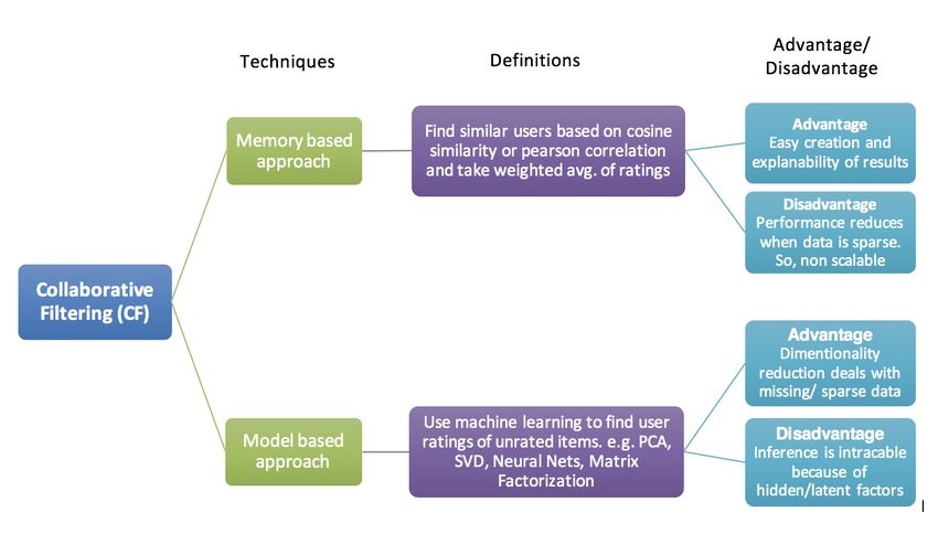
usually done through heuristics and recently through unstructured information, such as using
Latent Dirichlet Allocation (LDA) to compare texts.” [5]

Collaborative Filtering
As opposed to the aforementioned Content-Based Filtering, Collaborative Filtering employs only a
user’s past activity, e.g., past ratings, search queries, browsing history or purchases.

“Collaborative Filtering analyzes relationships between users and interdependencies among
products to identify new user-item associations” [4]. This format stems from the human custom of
asking friends and relatives with similar tastes for recommendations [5]. The more users interact
with items, the more accurate the recommendations become.

“Thanks to its simplicity -only requires a (User, Item, Rating) 3-tuple- and performance,
Collaborative Filtering is the most commonly used method. The information is commonly
represented in User-Item-Rating or User-Item Interaction matrices, which are almost always sparse
since it is highly common for there to be a very large number of items for any one user to rate” [5]
(picture one person watching the entire Netflix catalogue; extremely unlikely, if not impossible).

Two main methods can be distinguished: Memory-based and Model-based [5] as seen in Figure 4
and Figure 5 below.

 Figure 4. Breakdown of the two approaches to Collaborative Filtering [6]

 8

Figure 5. Overview of the Collaborative Filtering methods paradigm [3].

Memory-based methods
Also known as neighbourhood methods. Recommendations are built directly upon the ratings’
matrix. They consist of user-based and item-based methods.
 ● User-based: Also known as user-user. A user X’s recommendations will depend upon
 similar users’ ratings on items which X has not yet rated as seen in Figure 6 and Figure 7.
 Similarity amongst users can be calculated by finding users with similar ratings for a wide
 selection of items.

 Figure 6. Example of the user-user KNN method [3]

 9

Figure 7. User-oriented neighbourhood method. A prediction for Joe is obtained from the other 3 users deemed
 similar to him, who liked movies #1-4 [4].

 ● Item-based: Also known as item-item. A user X’s recommendations will depend upon their
 own ratings, and the system will recommend items akin to those already rated, such as in
 Figure 8. Similarity amongst items can be obtained by delineating items’ key features, or
 by grouping them according to how the majority of users interacted with each of them.

 Figure 8. Example of item-item KNN method [3]

“[…] item-based methods have better results overall since the similarity between items (is) more
reliable than the similarity between users. Imagine that after a while Alice can change her
preferences and ratings and this causes the poor performance in user-based methods. Shortly,

 10

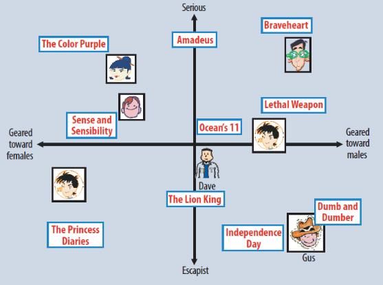
item-based methods are more stable with changes and rely on the items which tend to change
(less) than users.” [7]

In the majority of cases with the user-user methods, each user will have interacted with a limited
number of items, making them very susceptible to individual recorded interactions (high variance)
but more personalised (low bias). The opposite is true with item-item methods (low variance, high
bias).

Overall, KNN (K-Nearest Neighbours) is the most popular implementation, where the k most similar
users or items to a particular one are sought after in order to derive recommendations based upon
them. Approximate Nearest Neighbours (ANN) is also employed, especially with larger datasets.
The major problem with these Recommendation Systems is complexity and lack of scalability. As
part of a greater system with millions of users and/or items, constantly calculating nearest
neighbours can be a herculean task. Another issue comes from the “rich get richer” problem where
the same popular items are recommended to everyone, or where users get stuck into “information
confinement areas” where very similar items to the ones they already like are recommended, and
new or disruptive ones have no chance (they aren’t deemed “close enough neighbours”) [3].

A overview of each type can be seen in Figure 9:

 Figure 9. Contrast between user-based and item-based memory methods [3].

Model-based methods
 Also known as latent factor models. Recommendations are obtained from a model of the ratings’
matrix. “[...] (these approaches) assume an underlying “generative” model that explains the user-
item interactions and try to discover it in order to make new predictions” [3]. A very simplistic and
human-understandable example of this can be seen in Figure 10.

 11

The best-performing models are usually based on Matrix Factorisation, which presents the
hypothesis that users’ ratings are conditioned to an array of hidden factors inherent to the type of
items being rated, and thus the user-item interaction matrix is divided into 2 dense matrices: the
user-factor and the factor-item matrices. A more detailed look into this topic is provided later in
this document.

“[Matrix-factorisation methods] compress the user-item matrix into a low-dimensional
representation in terms of latent factors. One advantage of using this approach is that instead of
having a high dimensional matrix containing an abundant number of missing values we will be
dealing with a much smaller matrix in lower-dimensional space [...] There are several advantages
with this paradigm. It handles the sparsity of the original matrix better than memory-based ones.
Also comparing similarity on the resulting matrix is much more scalable [...].” [2]

 Figure 10. An example of a latent factor model, classifying both users and items on the same axes [4].

Despite generally bringing superior results in comparison to Content-Based Filtering [4], there is a
major downside to Collaborative Filtering: the cold start problem.

The cold start problem
The cold start problem or simply, cold start, refers to the inability to recommend items to new
users or to recommend something new to an existing user due to lack of sufficient information.

Note that this problem can occur in Content-based Filtering when a user with new, never-seen-
before features is presented, but generally speaking such an event rarely happens, and it is much
more predominant in Collaborative Filtering.

There is an array of possible solutions [3]:
 ● Random strategy: recommending random items to new users or new items to random
 users.

 12

● Maximum expectation strategy: recommending popular items to new users or new items
 to most active users.
● Exploratory strategy: recommending a set of various items to new users or a new item to a
 set of various users.
● Using a non-collaborative method for the early life of the user or the item, such as a
 survey.

 13

Evaluating Recommender Systems
Evaluation can be divided into two categories: based on well-defined metrics and based on
satisfaction estimation [3]. Evaluating Recommender Systems is not an easy task as of today, and
all in all, it is often recommended to use a combination of both types to ensure the best possible
RS [8].

Evaluation based on well-defined metrics
Akin to other Machine Learning models, if the output results in a clear numeric value, existing error
measurement metrics can be used (such as MAE, MSE or RMSE). These measure the quality of the
predictions [9].

A train-test split, dividing the dataset into training and testing subsets would have to be performed
and calculations done based upon those results. For this purpose, both the items and the users
could be divided, meaning two different train-test splits could have to be carried out, depending
on the paradigm used. In the case of Model-based Collaborative Filtering, for example, dividing by
users would not make sense since that would simply create cold-start problems for all those users
not previously seen by the model, and thus only splitting the items would be sensible.

Mean Absolute Error is a measure calculated from the absolute difference of each prediction and
the actual value, averaged out. The lower, the better. The formula is as follows:

 ∑ =1| − ̂ |
 =
 
Mean Squared Error is a measure obtained from the average of squared differences of each
prediction and the actual value. Root Mean Squared Error takes the square root of the result.
Because of the square, these metrics are much more susceptible to extremes, whereas MAE treats
all errors as equals. The lower, the better. The formulae are as follows:

 ∑ =1( − ̂ )2
 =
 
 ∑ =1( − ̂ )2
 = √
 
Another set of metrics that can be used are AUC-ROC, F1 Score, Accuracy, Precision or Recall,
depending on the nature of each problem. These measure the quality of the set of
recommendations [9]. They are all metrics derived from the Confusion Matrix (seen in Figure 11.
The Confusion Matrix .), which tallies the number of True Positives, True Negatives, False Positives
and False Negatives predicted (a TPs and TNs are the number of samples correctly classified as a
specific value in a binary classification, and FPs and FNs are samples incorrectly classified as one

 14

class when it was actually the other). The video in [11] explains these concepts in more detail, as
well as the example in [10].

 Figure 11. The Confusion Matrix [10].

AUC-ROC is based upon the curve of True Positive Rate, or Sensitivity, against False Positive Rate,
or 1-Sensitivity.

 = = , = 1 − =
 + + 

The line where the TPR and FPR are the same means all the cases that had to be classified as X
were, but all those that had to be classified as Y, weren’t, meaning everything was classified as X.
The farther the distance above that line, the better the model is. Anywhere below it signifies an
awful model.

Accuracy is the ratio between correct predictions to total predictions, the higher, with 1 being best
and 0, worst:

 + 
 =
 + + + 
Precision is the ratio between true positive predictions to total (both true and false) positive
predictions. In other words, out of those predicted as positive, how many were actually positive,
with 1 being best and 0, worst:

 =
 + 
Recall is the ratio between true positive predictions to what should have been positive predictions.
In other words, out of those that should have been classified as positive, how many were actually
classified as such, with 1 being best and 0, worst:

 15

 
 =
 + 
F1 Score is the balance between precision and recall, with 1 being best and 0, worst. Generally
speaking, it indicates an overall score for a classification model:

 ⋅ 
 1 = 2 ⋅
 + 

Finally, measures regarding the quality of the list of recommendations, such as Half-Life, or
Discounted Cumulative Gain (DCG), can be applied, although they are less common since they
require a larger number of recommendations [9].

“Half-life utility metric attempts to evaluate the utility of a ranked list to the user. The utility is
defined as the difference between the user’s rating for an item and the “default rating” for an item.
The default rating is generally a neutral or slightly negative rating. The likelihood that a user will
view each successive item is described with an exponential decay function, where the strength of
the decay is described by a half-life parameter” [12]. The overall utility of an RS is determined by ,
and each user’s utility is represented by . The formulae are as follows:

 max( , − ⅆ, 0)
 = ∑
 2( −1)∕( −1)
 
 = 100
 max
“Discounted Cumulative Gain is a measure of ranking quality. […] DCG measures the usefulness,
or gain, of a document based on its position in the result list. The gain is accumulated from the top
of the result list to the bottom, with the gain of each result discounted at lower ranks. […] Two
assumptions are made in using DCG and its related measures.

 1. Highly relevant documents are more useful when appearing earlier in a search engine
 result list (have higher ranks)
 2. Highly relevant documents are more useful than marginally relevant documents, which
 are in turn more useful than non-relevant documents.

[…] The premise of DCG is that highly relevant documents appearing lower in a search result list
should be penalized as the graded relevance value is reduced logarithmically proportional to the
position of the result.” [13]
The formula is as follows:

 16

 
 
 = ∑
 log 2 ( + 1)
 =1
Where is the graded relevance of the result at position , and , each of the results in the order
provided.

Overall, most, if not all, of the mentioned metrics ought to be considered and the corresponding
ones most useful for the domain of each specific instance should be afforded higher weights [14].

Evaluation based on beyond-accuracy metrics
In addition to quantitative, industry-standard metrics, other, more subjective ones, known as
beyond-accuracy metrics, can (and should) be applied, since the final target and consumer of
recommendations are humans, and thus what may seem like a good suit in data may in fact be
very repetitive, or even completely wrong (see Demographic Filtering). Therefore, metrics such as
Diversity, Coverage, Novelty, Serendipity, as well as Reliability or Explainability, among others, are
sought after once a model has proven quality results on paper [1, 3, 9, 15].
 • Diversity: How different results are from each other. How wide the spectrum of
 recommendations is. The degree of differentiation among recommended items.
 • Coverage: Proportion of items being recommended out of the total. Are the same items
 being recommended to every user or are a wide variety of items being recommended.
 • Novelty: How “new” or “never-seen-before” the results are in comparison with previous
 ones. The degree of difference between the items recommended to and known by the
 user.
 • Serendipity: Unexpectedness multiplied by relevance. The feeling of novelty and diversity
 without being irrelevant. Are users being stuck in “confinement areas”.
 • Reliability: How often is the model correct at suggesting new items.
 • Explainability: Can it be understood why the model recommended a certain item. “This
 movie was recommended to you because you liked Star Wars”, “people interested in this
 item also looked at”.

Keep in mind these do not necessarily have an agreed-upon method of being calculated, and for
each one metric, several formulae might have been proposed. Ultimately, it falls upon the
implementation team to decide which one best suits the problem at hand.

 17

Overview & State of the Art
The following figure depicts a summary of the information provided above, in a more graphical
manner:

 Figure 12. Overview of the different paths of RS implementations and their relationships [9]

 18

It is common nowadays to employ hybrid RSs for large-scale, commercial applications, since they
can offer more in-depth recommendations and efficiently work with extensive volumes of data,
such as those mentioned in Netflix or Amazon: “[…] (hybrid filtering methods) that combine
collaborative filtering and content-based approaches achieve state-of-the-art results in many
cases and are, so, used in many large-scale recommender systems nowadays. The combination
made in hybrid approaches can mainly take two forms: we can either train two models
independently […] and combine their suggestions or directly build a single model (often a neural
network) that unifies both approaches by using […] prior information (about user and/or item) as
well as “collaborative” interactions information.” [3]

However, it has proven difficult to answer “what is the state-of-the-art algorithm(s)” since a major
sticking point for RSs is reproducibility. Generally speaking, a large number of RSs (for example, 11
out of 18 neural recommendation algorithms as mentioned in [16]) cannot be used outside of the
domain they were built for, and those that can tend to imply certain “buts”, normally a worse
performance than simpler, more generalist ones: “In short: none of the 18 novel algorithms lead to
a real improvement over a relatively simple baseline” [16]. Thus, the only possibility that remains
at the time is to test out out-of-the-box implementations (“throwing things at the wall and seeing
what sticks”) and to analyse trends and existing approaches in order to tailor the RS for the
intended target and goal, instead of focusing on perfect replicability of existing complex
algorithms.

One of these trends is a growing interest in Recommender Systems capable of suggesting more
diverse, innovative and novel results, even at the expense of accuracy and/or precision. For this
purpose, the aforementioned satisfaction, or beyond-accuracy metrics, are prime [9]. This is
precisely some of the information which the model proposed by Lara-Cabrera et al. [1] can provide
in a more reliable manner than other models cannot, and a major reason for the implementation
of said model as the core of this project.

There is also interest in explaining recommendations in general, but even more so in a manner the
end-user easily understands to improve the reception they may have to said results, or, according
to Bobadilla et al. [9]: “this is an important aspect of an RS because it aids in maintaining a higher
degree of user confidence in the results generated by the system.” There are 4 main types of
explanations [9]:
 1. Human style explanations (user to user approach). For example, we recommend movie 
 because it was liked by the users who rated movies , , , . . . very positively ( , , , . . .
 are movies rated well by the active user).
 2. Item style explanations (item to item approach). For example, we recommend the
 vacation destination because you liked the vacation destinations , , , . . . ( , , , . . . are
 vacation destinations similar to and rated well by the active user).
 3. Feature style explanations (it is recommended based on items’ features). For example, we
 recommend movie because it was directed by director ⅆ, it features actors , , and it
 belongs to genre (ⅆ, , , are features the active user is interested in).
 4. Hybrid methods. This category primarily includes the following: human/item,
 human/feature, feature/item, and human/feature/ item.

A clear steering of the industry towards the addition and adaptation to multiple and varied types
of data in order to know the subjects better and to allow for finding more features previously
“invisible” to the existing models is taking place as well. Through this approach, recommendations
can be hyper-personalised, in line with the clear divergence away from primitive methods such as

 19

the original Demographic Filtering. According to Bobadilla et al., this runs “parallel to the
evolution of the web, which we can define through the following three primary stages:

(1) at the genesis of the web, RSs used only the explicit ratings from users as well as their
demographic information and content-based information […].
(2) For the web 2.0, in addition to the above information, RSs collect and use social information,
such as friends, followers, followed […]. Users aid in the collaborative inclusion of such
information: blogs, tags, comments, photos and videos.
(3) For the web 3.0 and the Internet of things, context-aware information from a variety of devices
and sensors will be incorporated with the above information. […] The expected trend is gradual
incorporation of information, such as radio frequency identification (RFID) data, surveillance data,
on-line health parameters and food and shopping habits, as well as teleoperation and
telepresence.” [9]

What this leads to are known as Context-aware Recommender Systems, which build upon the
contextual information mentioned above, such as location-aware models, widely extended and
used today, or bio-inspired models, which employ Genetic Algorithms (GAs) and Neural Networks
(NNs) models.

By relying on IoT and 5G, massive amounts of data can be elicited and used to find patterns,
habits, needs and desires the users themselves may not even be consciously aware of. This, of
course, raises a privacy and sensitivity concern, as the data being obtained is more and more
personal and thus requires a much more cautious treatment and handling, as well as becoming
increasingly precious to potential attackers. [9]

In a more practical aspect, a few frameworks, generally as Python modules (although Java, C++
and even C# libraries can also be found), are often used for general Machine Learning purposes,
including Recommender Systems, such as sklearn, Google’s TensorFlow or DeepCTR as well as RS-
specific ones the likes of CaseRecommender, OpenRec, TensorRec or python-recsys [17, 18, 19].

RSs can also come as a Software as a Service (SaaS) -also known as Recommendations-as-a-
Service or RaaS- product for easier integration within existing databases and systems as seen in
[20, 21] such as Universal Recommender, Yusp, Strands, or inbuilt services within Amazon’s AWS or
Microsoft’s Azure Cloud.

In [22] an array of different datasets with their best-performing RSs can be found. This is a much
more specific source, more likely less adaptable to concrete needs and a great point to browse
different papers at the current cutting-edge of innovation which may soon become mainstream, or
which could be a starting point and/or an inspiration for other RSs.

 20

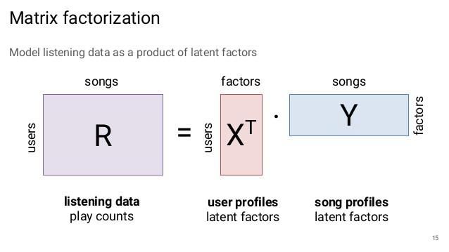
A Closer Look to Matrix Factorisation (MF)
Matrix Factorisation is a type of Model-based Collaborative Filtering approach where the user-item
interaction matrix is decomposed into 2 new matrices: the user-factor, and factor-item matrices,
which, through the dot-product, restore the user-interaction matrix again. This achieves the major
milestone of turning a sparse matrix into 2 dense ones as seen in Figure 13 and Figure 14, which is
far more efficient from a computational standpoint, although it introduces a slight reconstruction
error and extra storage space requirements.

 Figure 13. The matrix factorisation method [3]

 Figure 14. Another look at Matrix Factorisation [23]

 21

In the following example from Google [24], a coordinates system has been setup in Figure 15,
placing both users (based on their interests) and films (based on their characteristics) on a
spectrum of Children Adult (X axis), and Arthouse Blockbuster (Y axis).

 Figure 15. Positioning each user and item in a factor coordinate system [24].

This is then translated into a matrix of user-item interactions in Figure 16, where the
characteristics of each user and film in the form of coordinates are indicated with their own
matrices, and the explicit ratings are noted. It is then questioned whether the 4th user will enjoy
the film Shrek.

 Figure 16. Extraction of features/factors for both users and items [24]. The checks indicate a film the user has
 explicitly rated positively.

 22

For that, they make use of the two matrices mentioned before, known as the user-factor and
factor-item matrices (Figure 17), from which it is derived the user would not like Shrek (-0.9 score
out of a possible range of [-2, 2]). In fact, all the movies the different users would enjoy in this
example seem to be the ones they have already rated positively.

 Figure 17. Application of Matrix Factoring to obtain recommendations [24]. The squares with blue numbers
 (positive) indicate favourable ratings.

In this scenario the factors were provided manually, so as to make for an illustrative example, easy
to grasp for humans. As previously mentioned, finding those factors would be a task the model
itself would normally take care of, and instead of being human-understandable, they would likely
be of a purely mathematical nature:

“For example, consider that we have a user-movie rating matrix. In order to model the interactions
between users and movies, we can assume that:
 • There exist some features describing […] movies.
 • These features can also be used to describe user preferences (high values for features the
 user likes, low values otherwise).

However, we don’t want to give explicitly these features to our model […]. Instead, we prefer to let
the system discover these useful features by itself […]. As they are learned and not given,
extracted features taken individually have a mathematical meaning but no intuitive interpretation
(and, so, are difficult, if not impossible, to understand for humans). However, it is not unusual to
end up having structures emerging from (this) type of algorithm being extremely close to intuitive
decomposition that (a) human could think about.” [3]

Matrix Factorisation can be done through various methods, such as orthogonal factorization (SVD
simply tries to decompose the original matrix into 3 matrices, , where is a diagonal matrix,
and U and V are × and × complex unitary matrices, by minimising a given loss function,
usually the squared error, and the improved SVD++, since SVD cannot work with undefined or
NA/NaN values) [25], probabilistic factorization (PMF) that can be seen as “a probabilistic extension
of SVD which works well even when most entries in R are missing” and provides a probability
distribution instead of a concrete rating given feature vectors for users and items [26, 27], or non-
negative factorization (NMF and BNMF), where a non-unique decomposition of the original data is
obtained based on no negative values existing in the original data or by substituting all negative
values for a non-negative value, thus the name [1, 6, 28, 29]. Such level of detail falls outside the
scope of this project, but it must be noted that each may result in different factors being inferred
from the same sets of items, and thus different recommendations. Once again, no two RSs will
serve the same purpose and it’s why each ought to be calibrated for the desired results.

 23

“Matrix factorization models are superior to classic nearest-neighbour techniques for producing
product recommendations, allowing the incorporation of additional information such as implicit
feedback, temporal effects, and confidence levels.” [4] For this reason, and given the trend for
more varied data and explainability of the recommendations mentioned above, this can be
extremely useful and one of the reasons for the decision to work with a model of this kind for the
purpose of this project.

 24

The BeMF Model
BeMF stands for Bernoulli Matrix Factorisation [1], which is an RS model based upon the
assumption that the input data can be represented through a Bernoulli probability distribution: a
discrete distribution wherein two possible outcomes labelled by = 0 and = 1 in which = 1
("success") occurs with probability , and = 0 ("failure") occurs with probability ≡ 1 − ,
where 0 < < 1 [30].

This approach differs from the usual regression models, wherein the exact rating a user would give
to an item is predicted with a certain confidence; and instead, focuses on classifying each possible
outcome and its individual probability. This fact allows the modelling of the behaviour of the input
through a Bernoulli distribution by looking at each classification as a binary decision with
probability of the item falling into that class as seen in Figure 18, hence the name of the model.

 Figure 18. Information flow through the BeMF model [1].

The example provided in Lara-Cabrera et. al [1] mentions the DataLens dataset (an open dataset
commonly used for ML research and Proof-of-Concepts or PoCs) and the task of finding the
probability of a dichotomous classification: whether the user will give a rating of X to a certain
movie or not for each possible rating (1 to 5 stars). With this, the result comes out as a 5-element
vector, each element being the probability that the user will rate said movie with that rating. In
Figure 18 we can observe the user u would most likely rate the movie i with 4 out of 5 stars, with a
forecasted probability of 60% of this event happening (note the sum of probabilities adds to 1).

 25

The ability of providing a vector of probabilities/decisions as opposed to a single value (which it
can still do if so desired) gives a much better insight into how the model is recommending each
item and thus gives better explainability of results as well as using beyond-accuracy metrics with
each of the values. In a way, what is looked for is not if a user likes a certain item , but rather
how much do they like it. Therefore, said user has different factors for that item for each of the
ratings, although it is to be expected that the factors for any one rating to be similar to those for
ratings ± 1.

One downside of this process is the fact that the same work (updating the factors for each user
and item) is done for as many possible scores as there are available. If this work is parallelised, it
should not imply a major loss of efficiency, but parallelisation and threading tends not to be a
trivial task and usually requires high-level of knowledge and care to avoid race-conditions (where
two processes want to modify the same area of memory, and thus leads to incorrect values) and
other issues related to concurrency. Therefore, if considering a large number of ratings, this model
may not be suitable. That being said, users are usually restrained to simple and clear rating values,
such as the popular like-dislike or 1-5 stars, in order to ease rating and thus increase likelihood of
users carrying out that activity.

Another smaller downside is the fact that it has not been implemented in any of the major ML
libraries and has to be done manually. Since it is a rather simple model from an algorithmic
standpoint, this ought not to be a problem, but it is still an extra step resources have to be diverted
into, and one carried out for this project. A Java implementation is available on GitHub [31] and as
part of the Collaborative Filtering for Java (CF4J) framework [32] [33].

 26

Procedure
A meeting was first scheduled to come up with a primigenial set of features which could prove
useful for the RS. After a brief discussion, the following were chosen as good candidates for the
initial dataset given the ultimate use for it and the data already being collected:
 ● Geolocation
 ● Device type (OS, brand, model…)
 ● Service sought
 ● Age
 ● Gender

After careful study of the current capabilities by the Webel team, a first dump of 387
interactions/contracted services was provided, with the following columns:
 • 'id'
 • 'creationDate'
 • 'categoryID'
 • 'serviceType'
 • 'startDate'
 • 'endDate'
 • 'workAreaID'
 • (Redacted for privacy reasons)
 • 'serviceDuration'
 • (Redacted for privacy reasons)
 • 'clientID'
 • 'clientRegisterDate'
 • 'clientDeviceBrand'
 • 'clientDeviceModel'
 • 'clientDeviceSOVersion'
 • 'professionalID'
 • 'professionalRegisterDate'
 • 'professionalRating5'
 • 'professionalRating4'
 • 'professionalRating3'
 • 'professionalRating2'
 • 'professionalRating1'
 • 'professionalScore',
 • ‘rating’
 • ‘comment’

Note both age and gender couldn’t be used yet, but other valuable information not originally
considered was added instead. This data will be mostly used in the confines of cold-start problem-
solving, not for the model itself which only makes use of the User-Item ratings’ matrix.

In order to develop the model and perform all the data analysis and processing, a tool very
commonly used in Data Science was employed: a Jupyter Notebook, a tool for writing blocks of
code that can be executed in any order and interleaved with text for more descriptive explanations
including images, tables, graphs… In addition, a virtual environment was set up for increased
portability and ease of use and integration with the aid of the venv tool included in Python3. With
it, the required libraries and frameworks are already included, regardless of the destination

 27

computer’s setup. All that is therefore required is Python 3, and the virtual environment remains
self-contained.

Tool installation and environment setup
Installing the necessary libraries depends on the target device’s OS. Everything shown will be done
for a Microsoft-based PC, although the following steps can also be done on any Linux distribution
or MacOS device.

Python 3.6 or greater is required for the following process. To install, simply navigate to
https://www.python.org/downloads/ and download one of the suitable versions.

Next, open a Terminal and navigate to the folder where the project was downloaded. Run
./TFGEnv/Scripts/Activate.ps1 for PowerShell or ./TFGEnv/Scripts/activate.bat if using cmd to
activate the aforementioned virtual environment.

With that, the virtual environment should now be active, containing all the required modules.
Simply run jupyter notebook --autoreload and a tab should open in your browser. To open the
notebook, click on the .ipynb file and the project will open.

Should the /TFGEnv directory be missing, the modules can be installed by creating and activating
a new virtual environment and thanks to the requirements.txt file. In the base directory of the
project do:

pip install virtualenv # Should you not have it yet
python -m venv 
pip install -r ./requirements.txt

The main modules are NumPy [34], Pandas [35], Matplotlib [36] and Scikit-learn [37].

Practical work
Note: Instructions and indications are present in the Notebook itself for each of the steps and
sections, often similar or even more detailed than the ones present here. This document is aimed
to be a small reference or “quick-guide” more so than a detailed explanation.

The steps taken were customary of an ML project, first with data processing, followed by model
training and finally, evaluation. Exceptionally, synthetic data generation and model
implementation were also included prior to model training since this case required both of them.

For starters, the raw data, found in a .csv file, was loaded through Pandas, and an initial simple
preprocessing was performed, such as eliminating columns not relevant for the final product
either because they were purely internal (such as id, professionalScore), because they were
hidden to the user or didn't give any value when it came to predicting which professional a user is
more likely to hire (clientRegisterDate, clientDeviceBrand...), or simply because they could be
inferred from other columns (endDate).

The data types were also inferred as well as explicitly stated for each column in order to correctly
display the desired plots and be able to apply data-specific functions. The rating, categoryID and

 28

workAreaID columns were visualised in order to determine if further conclusions could be drawn
or if additional preparation was required.

 Figure 19. Original ratings' distribution

 Figure 20. Original categoryIDs’ distribution

 29

Figure 21. Original workAreaIDs' distribution

A total of 46 unique workAreaIDs, 77 *REDACTED*, 185 clientIDs and 141 professionalIDs were
present in the dataset, which served as a benchmark for the subsequent data generation.

Synthetic data generation (Data augmentation)
As mentioned above, not enough data is present, and since this is a bespoke solution, there is no
open-source alternative, so synthetic data had to be generated from the original dataset. For this,
random rows were chosen (with a uniform probability) for each one of the columns in order to
shuffle the existing information, creating 25,000 fictional hires that still followed the existing
distributions, as seen in Figure 22, Figure 23 and Figure 24. The possibility of creating new client
and professional IDs is given, as well as customising how many rows and new IDs to create.

 Figure 22. Comparison between ratings (original left, synthetic right)

 30

Figure 23. Comparison between categoryIDs (original left, synthetic right)

 Figure 24. Comparison between workAreaIDs (original left, synthetic right)

The only resulting difference is 184 clientIDs instead of 185, and a difference in
professionalRatings added to provide a certain level of diversity (since some columns didn’t have
a single positive value and the vast majority were zeroes), achieved using multipliers of the
standard deviation of the existing columns. Everything else was kept almost identical, but quantity
of results can be observed to be significantly higher.

Note: This process of data analysis was initially carried out with the purpose of providing a solution
for the cold-start problem, but since Webel already had a working solution on their end, it was
ultimately deemed unnecessary. Therefore, the work here shown is not used for anything other
than pure data visualisation and analysis, not for recommendations.

The next step was to generate the User-Item matrix by dropping all columns but clientID,
professionalID and rating. Since a user could rate a professional twice, the dichotomy of using the

 31

latest rating or the average rating is presented, and the choice has been given to the user of this
tool. In this specific instance, the average was used.

With this matrix, the model could then be implemented. This was done on a separate BeMF.py
file, and imported within the Notebook. Using the score, the evolution of
the model training can be followed and the models, evaluated against each other.

A (manual) ⅆ ℎ is performed to find the best hyperparameter combination possible out of
the 4 being considered. It is recommended that this process is run several times for the real
application each time the model is to be trained (every few weeks or months at most would be
optimal).

Since the data provided is so scarce, and data augmentation has been performed on the same
information, the current model’s factors and evaluations cannot be taken for more than a PoC and
are not indicative of the real results the model can achieve. For that, consult [1]. The original data
is much too diluted (387 original rows in comparison to 25,000, 64.6 times smaller) and the metrics
are therefore low, as expected:
 • Precision: 0.001324653167152607 (higher is better)
 • Recall: 0.0919384057971015 (higher is better)
 • Coverage (threshold 3): 1.0 (1 = all items offered, 0 = none items offered)

Lastly, the trained model can be exported and loaded back using Python’s pickle module to avoid
having to go through the training phase every time. This saves time and allows for major
portability and ease of use and integration.

With this, the tool is ready for usage and the model can now be successfully deployed.

Instruction and integration
A meeting was set up with Webel on the 6th of May 2021 (Figure 25) in order to showcase the
results of the work and train them on how to make use of it. This meeting was done over Zoom due
to time and sanitary restrictions.

The event was about 1 h 25 minutes in length, and the entire workings of the project were shown
during the walkthrough: from an overview of the theoretical basis through how the model was
implemented and how the Jupyter Notebook worked up to how they could use the results, how
often to retrain the model, the ideal amount of minimum data before the model could provide
reliable results, how to perform a test-train split and even how they could improve it if they so
wished.

Finally, a copy of the work was given to them in a .zip format, along with my commitment to help
in the future the moment they decide to integrate it or carry out any changes.

 32

Figure 25. A screenshot of the meeting featuring Javier Ginés, CTO of Webel

Overall, the outcome of the meeting and the work done was highly satisfactory, as proven by the
email they sent congratulating the work done (in Spanish):

 Figure 26. The email Webel sent to indicate their satisfaction with the resulting product.

 33

Environmental & Social Impacts
Regarding Environmental impacts, it is widely known that AI and model training tends to be a
resource-heavy process, with millions of computations performed every second, usually carried
out by a GPU (or in some instances, several of them [38]) or TPU [39] thanks to vectorial and matrix
operations being hyper-optimised in said hardware. Said Processing Units tend to draw a lot of
power in order to function at their top performance, thus requiring a lot of electrical energy. One
example can be seen in [40]: “researchers at the University of Massachusetts Amherst analysed
various natural language processing (NLP) training models available online to estimate the energy
cost in kilowatts required to train them. Converting this energy consumption in approximate
carbon emissions and electricity costs, the authors estimated that the carbon footprint of training
a single big language model is equal to around 300,000 kg of carbon dioxide emissions. This is of
the order of 125 round-trip flights between New York and Beijing”.

As can be observed, Machine Learning tools are extremely powerful, but power-hungry as well.
Recommender Systems in particular are even worse in this aspect, since they are geared towards
consumption, not necessarily solving the climate problem we currently face as a species. This
possibility of aid is one of the major points in favour of the advancement of AI despite its
(potentially massive, [41]) associated costs, as it could be one of the major keys to develop more
environmentally-friendly systems of all types, not just software ones. Therefore, RSs in general
tend to only feed into the problem, and not necessarily solve it, and it is a fact that should be
considered when deciding to employ one for a software application.

For this particular case it is not expected that training the model will poise a great threat to the
environment in any shape or form for as long as Webel remains a small company, and even if they
managed to scale up to a multi-million dollar operation, with hundreds of thousands or even
millions of users, by that time it is to be expected that they will have developed their own
customised model to better suit their needs.

On the Social side, one hugely influential Recommender Algorithm is YouTube’s, commonly
referred to by YouTubers in their videos when mentioning actions that said algorithm classifies as
“positive”, which cause the video to be shown to a wider audience and the creator(s) to reap in a
higher view count along with the associated benefits (money, exposure, influence…). This
algorithm has been the reason why many creators have either quit or become huge stars, all
depending on whether their content and how audiences interacted with it appeased or not said
algorithm at the time, as it has seen several different iterations as the website’s ecosystem
evolved. An example of this is the news channel Philip DeFranco, who oftentimes has been forced
to censor or outright cut out news from his daily online show due to the repercussions that not
doing so could have in his revenue, such as in [42]. In this particular case, it is not only DeFranco’s
livelihood at stake, but all of the staff who works for him, and this is far from an isolated case as
more and more YouTubers hire professionals to aid them with their content.

There’s also the user’s side to this, as Recommendation Systems almost dictate the content said
users consume. Look no further than TikTok’s infamous algorithm, one of the most powerful and
engaging, which consistently manages to hook in teenagers and adults alike by catering to their
specific interests for hours on end by learning from their activity. This has lent the Chinese app to
become the biggest social network in the year 2020, and one of the most used globally in the world
with an estimated 690 M active users in 2021 and over 2 thousand million downloads globally in 4
years, according to [43]. Because of this, the app has faced backlash over Hong Kong protest
censorship [44] and private data sharing with the Chinese Communist Party (CCP), including a

 34

potential ban on US territory for these actions. Amazon and their products are another similar
example, since they can dictate what products become popular or not, with all the financial
implications such ability entails.

All in all, having a say in what millions of people around the world are exposed to or not is a
massive power, with deep ramifications and consequences, and a highly coveted one, too. This is a
problem yet to be resolved which constantly plagues headlines all around the world and gives
Recommender Systems a bad image, since they are seen as tools of censorship and control
instead of search tools personalised to each individual’s needs.

In the case at hand, it is not expected for the BeMF model to cause problems of this sort, nor that it
will have any of the biases commonly present in people-recommending algorithms, such as racial,
geographical, political or religious, since none of these factors are taken into account when
training it, only the users’ known interactions with each item and the derived factors from them;
and since it is believed it can improve the experience and ease of user-professional connections,
the pros far outweigh the cons, hence why it was decided to proceed and carry out this project.

 35