The SOPHIE search for northern extrasolar planets - XVI. HD ...
←
→
Page content transcription
If your browser does not render page correctly, please read the page content below
A&A 636, L6 (2020)
https://doi.org/10.1051/0004-6361/201937254                                                                             Astronomy
c ESO 2020                                                                                                               &
                                                                                                                        Astrophysics

                                                           LETTER TO THE EDITOR

                   The SOPHIE search for northern extrasolar planets
        XVI. HD 158259: A compact planetary system in a near-3:2 mean motion
                                 resonance chain
   N. C. Hara1? , F. Bouchy1 , M. Stalport1 , I. Boisse2 , J. Rodrigues1 , J.-B. Delisle1 , A. Santerne2 , G. W. Henry3 ,
    L. Arnold4 , N. Astudillo-Defru5 , S. Borgniet6 , X. Bonfils6 , V. Bourrier1 , B. Brugger2 , B. Courcol2 , S. Dalal7 ,
       M. Deleuil2 , X. Delfosse6 , O. Demangeon8 , R. F. Díaz9,10 , X. Dumusque1 , T. Forveille6 , G. Hébrard7,4 ,
M. J. Hobson11,12 , F. Kiefer7 , T. Lopez2 , L. Mignon6 , O. Mousis2 , C. Moutou2,13 , F. Pepe1 , J. Rey1 , N. C. Santos8,14 ,
                                     D. Ségransan1 , S. Udry1 , and P. A. Wilson15,16,7

        1
            Observatoire Astronomique de l’Université de Genéve, 51 Chemin des Maillettes, 1290 Versoix, Switzerland
            e-mail: nathan.hara@unige.ch
        2
            Aix Marseille Univ, CNRS, CNES, LAM, Marseille, France
        3
            Center of Excellence in Information Systems, Tennessee State University, Nashville, TN 37209, USA
        4
            Observatoire de Haute-Provence, CNRS, Aix Marseille Universitté, Institut Pythtéas UMS 3470,
            04870 Saint-Michel-l’Observatoire, France
        5
            Departamento de Matemática y Física Aplicadas, Universidad Católica de la Santísima Concepción, Alonso de Rivera 2850,
            Concepción, Chile
        6
            Univ. Grenoble Alpes, CNRS, IPAG, 38000 Grenoble, France
        7
            Institut d’Astrophysique de Paris, UMR7095 CNRS, Universitté Pierre & Marie Curie, 98bis boulevard Arago, 75014 Paris, France
        8
            Instituto de Astrofísica e Ciências do Espaço, Universidade do Porto, CAUP, Rua das Estrelas, 4150-762 Porto, Portugal
        9
            Universidad de Buenos Aires, Facultad de Ciencias Exactas y Naturales, Buenos Aires, Argentina
       10
            CONICET – Universidad de Buenos Aires, Instituto de Astronomía y Física del Espacio (IAFE), Buenos Aires, Argentina
       11
            Instituto de Astrofésica, Pontificia Universidad Católica de Chile, Av. Vicuña Mackenna 4860, Macul, Santiago, Chile
       12
            Millennium Institute for Astrophysics, Macul, Chile
       13
            Canada-France-Hawaii Telescope Corporation, 65-1238 Mamalahoa Hwy, Kamuela, HI 96743, USA
       14
            Departamento de Fésica e Astronomia, Faculdade de Ciências, Universidade do Porto, Rua do Campo Alegre, 4169-007 Porto,
            Portugal
       15
            Department of Physics, University of Warwick, Coventry CV4 7AL, UK
       16
            Centre for Exoplanets and Habitability, University of Warwick, Coventry CV4 7AL, UK
      Received 4 December 2019 / Accepted 10 March 2020

                                                                    ABSTRACT

      Aims. Since 2011, the SOPHIE spectrograph has been used to search for Neptunes and super-Earths in the northern hemisphere.
      As part of this observational program, 290 radial velocity measurements of the 6.4 V magnitude star HD 158259 were obtained.
      Additionally, TESS photometric measurements of this target are available. We present an analysis of the SOPHIE data and compare
      our results with the output of the TESS pipeline.
      Methods. The radial velocity data, ancillary spectroscopic indices, and ground-based photometric measurements were analyzed with
      classical and `1 periodograms. The stellar activity was modeled as a correlated Gaussian noise and its impact on the planet detection
      was measured with a new technique.
      Results. The SOPHIE data support the detection of five planets, each with m sin i ≈ 6 M⊕ , orbiting HD 158259 in 3.4, 5.2, 7.9, 12,
      and 17.4 days. Though a planetary origin is strongly favored, the 17.4 d signal is classified as a planet candidate due to a slightly lower
      statistical significance and to its proximity to the expected stellar rotation period. The data also present low frequency variations,
      most likely originating from a magnetic cycle and instrument systematics. Furthermore, the TESS pipeline reports a significant signal
      at 2.17 days corresponding to a planet of radius ≈1.2 R⊕ . A compatible signal is seen in the radial velocities, which confirms the
      detection of an additional planet and yields a ≈2 M⊕ mass estimate.
      Conclusions. We find a system of five planets and a strong candidate near a 3:2 mean motion resonance chain orbiting HD 158259.
      The planets are found to be outside of the two and three body resonances.

      Key words. planets and satellites: detection – planets and satellites: dynamical evolution and stability –
      planets and satellites: fundamental parameters – planets and satellites: formation – methods: statistical – techniques: radial velocities

 ?
     CHEOPS fellow.

                                                         Article published by EDP Sciences                                            L6, page 1 of 17
A&A 636, L6 (2020)
1. Introduction Table 1. Known stellar parameters of HD 158259.
Transit surveys have unveiled several multiplanetary systems
where the planets are tightly spaced and close to low order Parameter Value
mean motion resonances (MMRs). For instance, Kepler-80 (Xie Right ascension (J2000) 17 h 25 min 24s.05
2013; Lissauer et al. 2014; Shallue & Vanderburg 2018), Kepler- Declination (J2000) +52.7906◦
223 (Borucki et al. 2011; Mills et al. 2016), and TRAPPIST- Proper motion (mas y−1 ) −91.047 ± 0.055, −49.639 ± 0.059
1 (Gillon et al. 2016; Luger et al. 2017) present 5, 4, and 7 Parallax 36.93 ± 0.029 mas
planets, respectively, in such configurations. These systems are Spectral type G0
often qualified as compact, in the sense that any two subsequent V magnitude 6.46
planets have a period ratio below 2. Compact, near resonant con- Radius 1.21+0.03
−0.08 R
figurations could be the result of a formation scenario where the Mass 1.08 ± 0.1 M
planets encounter dissipation in the gas disk, are locked in res- v sin i 2.9 km s−1
onance, and then migrate inwards before potentially leaving the log R0hK −4.8
resonance (e.g., Terquem & Papaloizou 2007; MacDonald et al.
2016; Izidoro et al. 2017). Notes. Parallax, coordinates, proper motion, and radius are taken
Near resonant, compact systems are detectable by radial from Gaia Collaboration et al. (2018), spectral type is from
velocity (RV), as demonstrated by follow up observations of Cannon & Pickering (1993), and V magnitude is from Høg et al.
transits (Lopez et al. 2019). However, such detections with (2000). Mass is from Chandler et al. (2016).
only RV are rare: HD 40307 (Mayor et al. 2009) and HD
215152 (Delisle et al. 2018) both have three planets near 2:1 –
2:1 and 5:3 – 3:2 configurations, respectively.
HD158259 radial velocities (outliers removed)
In the present work, we analyze the 290 SOPHIE radial 13550
velocity measurements of HD 158259. We detect several signals,
13545
Velocity (m/s)
which are compatible with a chain of near resonant planets. The
signals have an amplitude in the 1−3 m s−1 range. At this level, 13540
in order to confirm their planetary origin, it is critical to consider 13535
whether these signals could be due to the star or to instrument
systematics. To this end, we include the following data sets in our 13530
analysis: the bisector span and log R0 HK derived from the spectra 13525
as well as ground-based photometric data. The periodicity search 56000 56500 57000 57500 58000 58500
is performed with a `1 periodogram (Hara et al. 2017) includ- Time (rjd)
ing a correlated noise model, selected with new techniques. The
Fig. 1. SOPHIE radial velocity measurements of HD 158259 after out-
results are compared to those of a classical periodogram (Baluev
liers at BJD 2457941.5059, 2457944.4063, and 2457945.4585 have
2008). been removed.
Furthermore, HD 158259 has been observed in sector 17 of
the TESS mission (Ricker et al. 2014). The results of the TESS
reduction pipeline (Jenkins et al. 2010, 2016) are included in our
analysis. 2.2. SOPHIE radial velocities
The data support the detection of six planets close to a 3:2
MMR chain, with a lower detection confidence for the outermost SOPHIE is an échelle spectrograph mounted on the 193cm
one. The orbital stability of the resulting system is checked with telescope of the Haute-Provence Observatory (Bouchy et al.
numerical simulations, and we discuss whether the system is in 2011). Several surveys have been conducted with SOPHIE,
or out of the two and three-body resonances. including a moderate precision survey (3.5–7 m s−1 ), aimed at
The Letter is structured as follows. The data and its analysis detecting Jupiter-mass companions (e.g., Bouchy et al. 2009;
are presented in Sects. 2 and 3, respectively. The study of the Moutou et al. 2014; Hébrard et al. 2016), as well as a search
system dynamics is presented in Sect. 4, and we conclude in of smaller planets around M-dwarfs (e.g., Hobson et al. 2018,
Sect. 5. 2019; Díaz et al. 2019).
Since 2011, SOPHIE has been used for a survey of bright
solar-type stars, with the aim of detecting Neptunes and super-
Earths (Bouchy et al. 2011). For all the observations performed
2. Data in this survey, the instrumental drift was measured and cor-
2.1. HD 158259 rected for by recording on the detector, close to the stellar spec-
trum, the spectrum of a reference lamp. This one is a thorium-
HD 158259 is a G0 type star in the northern hemisphere with a argon lamp before barycentric Jullian date (BJD) 2458181 and
V magnitude of 6.4. The known stellar parameters are reported a Fabry-Perot interferometer after this date. The observations of
in Table 1. The stellar rotation period is not known precisely, HD 158259 were part of this program. Over the course of seven
but it can be estimated. The median log R0hK , which was obtained years, 290 measurements were obtained with an average error
from SOPHIE measurements, is −4.8 ± 0.1. With the empirical of 1.2 m s−1 . The data, which were corrected from instrumen-
relationship of Mamajek & Hillenbrand (2008), this translates to tal drift and outliers (see Appendix A.1 and A.2), are shown in
an estimated rotation period of 18 ± 5 days. Additionally, the Fig. 1.
SOPHIE RV data give v sin i = 2.9 ± 1 km s−1 (see Boisse et al. The RV is not the only data product that was extracted from the
2010). Assuming i = 90◦ and taking the Gaia radius estimate of SOPHIE spectra. The SOPHIE pipeline also retrieves the bisec-
1.21 R , the v sin i estimation yields a rotation period of ≈20 ± 7 tor span (Queloz et al. 2001) as well as the log R0hk (Noyes et al.
days. 1984).
L6, page 2 of 17N. C. Hara et al.: The SOPHIE search for northern extrasolar planets. XVI
HD 158259 l1 periodogram, noise model with best cross validation score Table 2. Periods appearing in the `1 periodogram and their false alarm
probabilities with their origin, the semi-amplitude of corresponding sig-
nals, and M sin i with 68.7% intervals.
Peak period (d) FAP Origin K (m s−1 ) M sin i (M⊕ )
Detected by SOPHIE RV
3.432 2 × 10⁻⁵ Planet c 2.2+0.2
−0.2 5.5+0.5
−0.6
5.198 8 × 10⁻³ Planet d 1.9+0.2
−0.2 5.3+0.7
−0.7
7.954 1.6 × 10⁻³ Planet e 1.8+0.3
−0.3 6.0+0.9
−1.0
12.03 2.8 × 10⁻³ Planet f 1.6+0.4
−0.3 6.1+1.2
−1.3
17.39 2.3 × 10⁻² Candidate g 1.6+0.5
−0.3 6.8+1.8
−1.6
Fig. 2. `1 periodogram of the SOPHIE radial velocities of HD 158259 366 1.1 × 10⁻⁶ Systematic 3.4+0.7
−0.8 40+9
−10
corrected from outliers (in blue). The periods at which the main peaks 640 1.3 × 10⁻² Activity − −
occur are represented in red. 1920 2.1 × 10⁻² Activity 2.9+0.4
−0.4
Detected by TESS + confirmed by SOPHIE RV
2.177 0.44 Planet b +0.2
1.0−0.2 2.2+0.4
2.3. APT Photometry −0.4
Alias of 1.84 d, Radius: 1.2 ± 1.3 R⊕ , Density: 1.09+0.23
−0.27 ρ⊕
Photometry has been obtained with the T11 telescope at the Other signals
Automatic Photoelectric Telescopes (APTs), located at Fairborn 34.5 1.0 Candidate? – –
Observatory in southern Arizona. The data, covering four obser- 17.7 0.5 – – –
vation seasons, are presented in more detail in Appendix A.3.
2.4. TESS results as input. It aims to find a representation of the RV time series as
a sum of a small number of sinusoids whose frequencies are in
HD 158259 was observed from 7 Oct to 2 Nov 2019 (sector 17). the input grid. It outputs a figure which has a similar aspect as a
The TESS reduction pipeline (Jenkins et al. 2010, 2016) found regular periodogram, but with fewer peaks due to aliasing. The
evidence for a 2.1782 ±0.0006 d signal with a time of conjunc- peaks can be assigned a FAP, whose intrepretation is close to the
tion T c = 2458766.049072 ± 003708 BJD (TOI 1462.01). The FAP of a regular periodogram peak.
detection was made with a signal-to-noise ratio of 8.05, which The signals found to be statistically significant might vary
is above the detection threshold of 7.3 adopted in Sullivan et al. from one noise model to another. To explore this aspect, we con-
(2015). sidered several candidate noise models based on the periodic-
ities found in the ancillary indicators. The noise models were
ranked with cross-validation and Bayesian evidence approxima-
3. Analysis of the data sets tions (see Appendix B). In Fig. 2, we show the `1 periodogram of
3.1. Ground-based photometry and ancillary indicators the SOPHIE RVs corresponding to the noise with the best cross
validation score on a grid of equispaced frequencies between 0
If the bisector span, log R0HK , or photometry show signs of tem- and 0.7 cycle d−1 . The FAPs of the peaks pointed by red mark-
poral correlation, in particular, periodic signatures, this might ers in Fig. 2 are given in Table 2. They suggest the presence of
mean that the RVs are corrupted by stellar or instrumental signals, in decreasing strengths of detection, at 366, 3.43, 7.95,
effects (e.g., Queloz et al. 2001). To search for periodicities, 12.0, 5.19, 1920, 640 , and 17.4 days. The significance of the
we applied the generalized Lomb-Scargle periodogram itera- signals at 1.84, 17.7, and 34.5 d is found to be marginal to null.
tively (Ferraz-Mello 1981; Zechmeister & Kürster 2009) as well The FAPs reported in Table 2 were computed with a cer-
as the `1 periodogram (Hara et al. 2017) for comparison pur- tain noise model, which is the best in a sense described in
poses. The process is presented in detail in Appendix A.4. Appendix B. In this appendix, we also explore the sensitivity
The log R0Hk periodogram presents a peak at 2900 d with a of the detections to the noise model choice. We find the detec-
false alarm probability (FAP) of 4 × 10⁻¹² . This signal is the tion of signals at 3.43, 5.19, 7.95, and 12.0 d to be robust. The
only clear feature of the ancillary indicators, and it supports the detection of signals at 1920, 366, and 17.4 d is slightly less
presence of a magnetic cycle with a period >1500 d. We note strong but still favored. There is evidence for a 640 d signal
that both the APT photometry and bisector span present a peak and hints of signals at 34.5 d and 1.84 d or 2.17 d. The latter
around 11.6 d, though with a high FAP level. This periodicity as two are aliases of one another. Indeed, the RV spectral win-
well as other periodicities found in the indicators were used to dow has a strong peak at the sidereal day (0.9972 d), which
build candidate noise models for the analysis of the RVs, which is common in RV time series (Dawson & Fabrycky 2010), and
is the object of the next section. 1/1.840 + 1/2.177 = 1/0.9972 d−1 .
In Appendix C, the results are compared to a classical peri-
3.2. Radial velocities analysis odogram approach with a white noise model, which gives similar
results but fails to unveil the 1.84/2.17 d candidate in the signal.
The RV time series we analyze here was corrected for instrument We also study whether the apparent signals could originate from
drift and from outliers. The process is described in Appendix A.1 aliases of the periods considered here. This possibility is found
and A.2. To search for potential periodicities, we computed the to be unlikely.
`1 periodogram of the RV, as defined in Hara et al. (2017). This We fit a model with a free error jitter and nine sinusoidal
tool is based on a sparse recovery technique called the basis pur- functions initialized at the periods listed in the upper part of
suit algorithm (Chen et al. 1998). The `1 periodogram takes in Table 2. The data, which were phase-folded at the fitted peri-
a frequency grid and an assumed covariance matrix of the noise ods, are shown in Figs. 3 and 4. The error bars correspond to the
L6, page 3 of 17A&A 636, L6 (2020)
15
10
10
5
5
ΔRV [m/s]
ΔRV [m/s]
0
0
-5 -5
-10 -10
0 50 100 150 200 250 300 350 0 50 100 150 200 250 300 350
Mean Anomaly [deg] Mean Anomaly [deg]
Model SOPHIE(DRS-OHPc) Model SOPHIE(DRS-OHPc)
15
10
10
5
5
ΔRV [m/s]
ΔRV [m/s]
0
0
-5 -5
-10 -10
-15 -15
0 50 100 150 200 250 300 350 0 50 100 150 200 250 300 350
Mean Anomaly [deg] Mean Anomaly [deg]
Model SOPHIE(DRS-OHPc) Model SOPHIE(DRS-OHPc)
15
15
10
10
5
5
ΔRV [m/s]
ΔRV [m/s]
0
0
-5
-5
-10
-10
-15
-15
0 50 100 150 200 250 300 350 0 50 100 150 200 250 300 350
Mean Anomaly [deg] Mean Anomaly [deg]
Model SOPHIE(DRS-OHPc) Model SOPHIE(DRS-OHPc)
10 Fig. 4. Radial velocity phase-folded, from top to bottom, at: 360, 750,
5
and 2000 d.
ΔRV [m/s]
0
-5 obtained with a noise model that includes white and correlated
-10 components.
-15
0 50 100 150 200 250 300 350
Mean Anomaly [deg]
Model SOPHIE(DRS-OHPc) 3.3. Periodicity origin
15
10
The origin of the 366, 640, and 1920 d signals is uncertain, and
5
we do not claim planet detections at those periods. The 366 d sig-
ΔRV [m/s]
0
nal is fully compatible with a yearly signal. Instrument system-
-5
atics, such as the stitching effect (Dumusque et al. 2015), could
-10 produce this signal, and they are deemed to be its most likely
-15 origin. We fit a Gaussian process on the log R0HK and used it as a
0 50 100 150 200
Mean Anomaly [deg]
250 300 350 linear predictor on the RVs, similarly to Haywood et al. (2014).
Model SOPHIE(DRS-OHPc)
When computing the periodogram on the residuals of the fit,
15
there is no trace of signals in the 1500–3000 d and 600–800 d
10 regions, so they might stem from a magnetic cycle. The signal at
34.5 d could be a faint trace of a planet near the 2:1 resonance,
ΔRV [m/s]
5
0 but its significance is too low to be conclusive.
-5 The periods at 3.43, 5.19, 7.95, 12.0, and 17.4 d, which are
-10 significant in the RV analysis, most likely stem from planets.
0 50 100 150 200 250 300 350
Here, we list five arguments that support this claim. (i) None of
Model SOPHIE(DRS-OHPc)
Mean Anomaly [deg]
these periods clearly appear in the bisector span, log R0hk , or pho-
tometry. (ii) While eccentric planets can be mistaken for planet
Fig. 3. Radial velocity phase-folded at the periods of the signals appear- pairs near a 2:1 MMR, they are very unlikely to appear as planets
ing in the period analysis. From top to bottom: 2.17, 3.43, 5.19, 7.95,
near a 3:2 resonance (Hara et al. 2019). (iii) The periods could be
12.0, and 17.4 d.
due to instrument systematics. We find it unlikely since the peri-
ods of the planet candidates do not consistently appear in the 123
addition in quadrature of the nominal uncertainties and the fitted other data sets of the survey HD 158259 is a part of Hara et al.
jitter. (in prep.). (iv) All the signals are consistent in phase and ampli-
The residuals of the nine-signals model plus white noise fit tude (see Appendix D). (v) Most importantly, the period ratio of
have a root mean square (RMS) of 3.1 m s−1 , which is higher two subsequent planets is very close to 3:2, namely 1.51, 1.53,
than the nominal uncertainties of the SOPHIE data (1.2 m s−1 ). 1.51, and 1.44, and they have very similar estimated masses (see
We studied the residuals with the methods of Hara et al. (2019) Sect. 3.4). Pairs of planets close to the 3:2 period ratio are known
and found that they are temporally correlated, which, if not to be common (Lissauer et al. 2011a; Steffen & Hwang 2015),
accounted for, might corrupt the orbital element estimates. In and it seems unlikely that the stellar features would mimic this
Appendix E, we show that a consistent model of the data can be specific spacing of periods.
L6, page 4 of 17N. C. Hara et al.: The SOPHIE search for northern extrasolar planets. XVI
HD 158259 configuration from RV a correlated noise model with an exponential decay. The prior
at TESS estimated Tc on eccentricity was chosen to strongly disfavor e > 0.1 (see
0.15 Periods (d) Sect. 4 for justification). The details of the posterior calculations
2.17 are presented in Appendix E and the main features of the sig-
0.10 3.43 nals are reported in Table 2. Planets c, d, e, f , and planet can-
5.19 didate g exhibit m sin i ≈ 6 M⊕ and planet b has m ≈ 2 M⊕
line of sight (AU)
0.05 7.95 and R ≈ 1.2 R⊕ , which is compatible with a terrestrial den-
12.0 sity. The yearly signal has an amplitude of ≈3 m s−1 . We find
0.00 17.4 a significantly nonzero time-scale of the noise of 5.4+0.8 −2.6 d. A
more detailed analysis shows hints of nonstationary noises (see
0.05 Appendix D).
The TESS photometry exhibits a transit signal from b, but
0.10 not from c, d, e, f , or g. Given the masses of c, d, e, f , and g, their
transits should have been detected had they occurred. Assuming
0.15 To observer a coplanar system, this can be explained if the inclination departs
◦
0.15 0.10 0.05 0.00 0.05 0.10 0.15 from 90◦ from at least 7.08+0.36
−0.43 (so that the transit of c cannot be
x axis (AU) detected) to 9.5+0.57
◦
−0.48 at most (the transit of b must be seen). This
Fig. 5. Configuration of the system estimated from the RV at the time would translate to a sin i between 0.985 and 0.993. Alternately,
of conjunction estimated by TESS (BJD 58766.049072). the planets could be relatively inclined.
Signals at 12 and 17.4 d verify the five points listed above and 4. Dynamical analysis
are thus considered as planets. We, however, point out that the
4.1. Stability
predicted rotation period of the star is 18 ± 5 d. This means that
signals could be present in this period range, not necessarily at For the dynamical analysis of the system, we consider the plan-
the stellar rotation period or its harmonic (Nava et al. 2020). Fur- ets b, c, d, e, f, and candidate g, whose period ratios are close to
thermore, in Appendix B, we show that the 17.4 d signal is less the 3:2 MMRs: Pc /Pb = 1.57, Pd /Pc = 1.51, Pe /Pd = 1.53,
significant and that certain noise models favor 17.7 d over 17.4 d. P f /Pe = 1.51, and Pg /P f = 1.44. To check the existence of
It appears that fitting signals at 17.4 or 17.7 d does not com- stable solutions, we proceeded as follows. We performed the
pletely remove the other. This might point to differential rotation MCMC analysis with exactly the same priors as in Sect. 3.4
or dynamical effects, but it is most likely due to modeling uncer- except with a looser prior on eccentricity. Each MCMC sam-
tainties. Nonetheless, the nature and period of the 17.4 d signal ple was taken as an initial condition for the system. Its evo-
are subject to a little more caution than the other planets. It is lution was integrated 1 kyr in the future using the 15th order
thus conservatively classified as a strong planet candidate. N-body integrator IAS15 (Rein & Spiegel 2015) from the pack-
The 2.17 d signal appearing in TESS has a counterpart in age REBOUND1 (Rein & Liu 2012). General relativity was
the RVs, which appear at 1.84 d (alias) here. The RV signal is included via REBOUNDx, using the model of Anderson et al.
marginally significant but compatible with the observation of a (1975). In total, 36 782 system configurations were integrated.
transit. Indeed, the time of conjunction as measured by TESS We consider the system to be unstable if any two planets have an
is BJD 2458766.049072 ± 0.003708. At this epoch, the mean encounter below their mutual Hill radius. A total of 1700 sam-
longitude of the innermost planet predicted from the RV with a ples lead to integrations where the stability condition was not
◦
prior on the period set from TESS data is 95+23 −23 (see Sect. 3.4 violated. We computed their empirical probability distribution
for details on the posterior calculation). On this basis, the 2.17 d functions and found constraints on the eccentricities .0.1.
signal is considered to stem from a planet. We note that no trace
of the other planets is found in the TESS data.
In Fig. 5 we represent the configuration of the system at the 4.2. Resonances
time of conjunction given by the TESS pipeline. The markers The planets of HD 158259 could be locked in 3:2 or three body
represent the position of the planets corresponding to their pos- resonances. This would translate to the following conditions. We
terior mean (semi major axis and mean longitude). The marker consider three subsequent planets, indexed by i = 1, 2, 3 from
size is proportional to an estimated radius ∝ (m sin i)0.55 , fol- innermost to outermost. With λi , Pi , and $i , we denote their
lowing Bashi et al. (2017). The plain colored lines correspond to mean longitudes, periods, and arguments of periastron. In case
68% credible intervals on the mean longitude. of two body resonances, the angle
In summary, we deem six of the nine significant signals to
originate from planets: 2.17, 3.43, 5.19, 7.95, 12.0, and 17.4 d, ψ12 = 3λ2 − 2λ1 − $ j , j = 1, 2 (1)
with a slightly lower confidence in 17.4 d. From now on, they
are referred to as planets b, c, d, e, f , and (strong) candidate g, would librate. Following Delisle (2017), in case of three-body
respectively. resonances, the so-called Laplace angle
φ123 = 3λ3 + 2λ1 − 5λ2 (2)
3.4. Orbital elements
should librate around π. The posterior distributions of ψi j and
To derive the uncertainties on the orbital elements of the plan- φi jk as well as their derivatives were computed for any doublet
ets, we computed their posterior distribution with a Monte Carlo and triplet of planets from the MCMC samples, assuming that $ j
Markov chain algorithm (MCMC). The model includes signals
at 2.17, 3.43, 5.19, 7.95, 12.0, and 17.4 d, a linear predictor fit- 1
The REBOUND code is freely available at http://github.com/
ted on the log R0HK with a Gaussian process analysis, as well as hannorein/rebound.
L6, page 5 of 17A&A 636, L6 (2020)
is constant on the time-scale of the observations. We conclude acknowledges long-term support from NASA, NSF, Tennessee State University,
that the system is not locked in two and three body resonances. and the State of Tennessee through its Centers of Excellence program. X.De.,
We note that the circulation of the angles occurs at different rates, X.B., I.B., and T.F. received funding from the French Programme National de
Physique Stellaire (PNPS) and the Programme National de Planétologie (PNP) of
φcde being the slowest. CNRS (INSU). X.B. acknowledges funding from the European Research Coun-
Nevertheless, period ratios so close to 3:2 are very unlikely cil under the ERC Grant Agreement n. 337591-ExTrA. This work has been sup-
to stem from pure randomness. It is therefore probable that the ported by a grant from Labex OSUG@2020 (Investissements d’avenir – ANR10
planets underwent migration in the protoplanetary disk, during LABX56). This work is also supported by the French National Research Agency
in the framework of the Investissements d’Avenir program (ANR-15-IDEX-02),
which each consecutive pair of planets was locked in 3:2 MMR. through the funding of the ‘Origin of Life’ project of the Univ. Grenoble-Alpes.
The observed departure of the ratio of periods of two subse- V.B. acknowledges support from the Swiss National Science Foundation (SNSF)
quent planets from exact commensurability might be explained in the frame of the National Centre for Competence in Research PlanetS, and
by tidal dissipation, as was already proposed for similar Kepler has received funding from the European Research Council (ERC) under the
systems (e.g., Delisle & Laskar 2014). Stellar and planet mass European Unions Horizon 2020 research and innovation programme (project
Four Aces; grant agreement No 724427). This work was supported by FCT –
changes have also been suggested as a possible cause of res- Fundação para a Ciência e a Tecnologia/MCTES through national funds (PID-
onance breaking (Matsumoto & Ogihara 2020). The reasons DAC) by this grant UID/FIS/04434/2019, as well as through national funds
behind the absence of three-body resonances, which are seen (PTDC/FIS-AST/28953/2017 and PTDC/FIS-AST/32113/2017) and by FEDER
in other resembling systems (e.g., Kepler-80, MacDonald et al. – Fundo Europeu de Desenvolvimento Regional through COMPETE2020 –
Programa Operacional Competitividade e Internacionalizaȩão (POCI-01-0145-
2016), are to be explored. FEDER-028953 and POCI-01-0145-FEDER-032113). N.A-D. acknowledges
support from FONDECYT #3180063. X.Du. is grateful to the Branco Weiss
Fellowship–Society in Science for continuous support.
5. Conclusion
In this work, we have analyzed 290 SOPHIE measurements of References
HD 158259. The analysis of the radial velocity data, including a
correction of the instrument drift and over 7500 correlated noise Akaike, H. 1974, IEEE Trans. Autom. Control, 19, 716
Amelunxen, D., Lotz, M., McCoy, M. B., & Tropp, J. A. 2014, Inf. Inference J.
models, support the detection of four planets (c, d, e, and f ) and a IMA, 3, 224
strong candidate (g), with respective periods of 3.43, 5.19, 7.95, Anderson, J. D., Esposito, P. B., Martin, W., Thornton, C. L., & Muhleman, D.
12.0, and 17.4 d. They all exhibit a ≈6 M⊕ mass. There is sub- O. 1975, ApJ, 200, 221
stantial evidence for a planetary origin of the 17.4 d signal, and Baluev, R. V. 2008, MNRAS, 385, 1279
the remaining concerns on its nature should be cleared with a Bashi, D., Helled, R., Zucker, S., & Mordasini, C. 2017, A&A, 604, A83
Boisse, I., Eggenberger, A., Santos, N. C., et al. 2010, A&A, 523, A88
better estimate of the stellar period. Furthermore, the TESS data Borucki, W. J., Koch, D. G., Basri, G., et al. 2011, ApJ, 736, 19
exhibit a 2.17 d signal that is compatible with the RVs, which Bouchy, F., Hébrard, G., Delfosse, X., et al. 2011, EPSC-DPS Joint Meeting
allows one to claim the detection of an additional planet (b) and 2011, 2011, 240
to measure a density of 1.09+0.23
−0.27 ρ⊕ . The TESS photometry does
Bouchy, F., Hebrard, G., Udry, S., Delfosse, X., & Boisse, I. 2009, A&A, 505,
853
not show other transits. There exist stable configurations of the Cannon, A. J., & Pickering, E. C. 1993, VizieR Online Data Catalog: III/135A
six-planet system that are compatible with the error bars. Chandler, C. O., McDonald, I., & Kane, S. R. 2016, VizieR Online Data Catalog:
While many compact near-resonance chains have been J/AJ/151/59
detected by transits, they have been rare in radial velocity Chen, S. S., Donoho, D. L., & Saunders, M. A. 1998, SIAM J. Sci. Comput., 20,
surveys so far. The present analysis shows that they can be 33
Ciardi, D. R., Fabrycky, D. C., Ford, E. B., et al. 2013, ApJ, 763, 41
detected, provided there are enough data points and an appro- Courcol, B., Bouchy, F., Pepe, F., et al. 2015, A&A, 581, A38
priate accounting of correlated noises (instrumental and stellar). Dawson, R. I., & Fabrycky, D. C. 2010, ApJ, 722, 937
HD 158259 b, c, d, e, f , and g are such that subsequent Delisle, J.-B. 2017, A&A, 605, A96
planets have period ratios of 1.57, 1.51, 1.53, 1.51, and 1.44 Delisle, J.-B., & Laskar, J. 2014, A&A, 570, L7
Delisle, J.-B., Ségransan, D., Dumusque, X., et al. 2018, A&A, 614, A133
with increasing period. Subsequent planet pairs and triplets are Delisle, J. B., Hara, N. C., & Ségransan, D. 2019, A&A, submitted
close to, but not within, 3:2 and three-body mean motion res- Delisle, J. B., Hara, N., & Ségransan, D. 2020, A&A, 635, A83
onances. The period ratios are consistent with the distribution Díaz, R. F., Delfosse, X., Hobson, M. J., et al. 2019, A&A, 625, A17
of period ratios of planet pairs found in Kepler, which exhibits Dumusque, X., Pepe, F., Lovis, C., & Latham, D. W. 2015, ApJ, 808, 171
a peak at 1.52 (see Lissauer et al. 2011a; Fabrycky et al. 2014; Fabrycky, D. C., Lissauer, J. J., Ragozzine, D., et al. 2014, ApJ, 790, 146
Ferraz-Mello, S. 1981, AJ, 86, 619
Steffen & Hwang 2015). The similarity of the masses of the Foreman-Mackey, D., Agol, E., Ambikasaran, S., & Angus, R. 2017, AJ, 154,
planets of the system is compatible with the hypothesis that plan- 220
ets within the same system have similar sizes (Lissauer et al. Gaia Collaboration 2018, VizieR Online Data Catalog: I/345
2011b; Ciardi et al. 2013; Millholland et al. 2017; Weiss et al. Gillon, M., Jehin, E., Lederer, S. M., et al. 2016, Nature, 533, 221
Hara, N. C., Boué, G., Laskar, J., & Correia, A. C. M. 2017, MNRAS, 464, 1220
2018). The configuration of the planets can be explained Hara, N. C., Boué, G., Laskar, J., Delisle, J. B., & Unger, N. 2019, MNRAS,
by existing formation scenarios (e.g., Terquem & Papaloizou 489, 738
2007; Delisle & Laskar 2014). The proximity to 3:2 resonances Haywood, R. D., Collier Cameron, A., Queloz, D., et al. 2014, MNRAS, 443,
of the HD 158259 system is reminiscent of Kepler-80 2517
(MacDonald et al. 2016). However, the latter presents three- Hébrard, G., Arnold, L., Forveille, T., et al. 2016, A&A, 588, A145
Henry, G. W. 1999, PASP, 111, 845
body resonances, while HD 158259 does not. It would be Hobson, M. 2019, Exoplanet detection around M dwarfs with near infrared and
interesting to investigate scenarios that can explain the differ- visible spectroscopy
ences between the two systems. Hobson, M. J., Díaz, R. F., Delfosse, X., et al. 2018, A&A, 618, A103
Hobson, M. J., Delfosse, X., Astudillo-Defru, N., et al. 2019, A&A, 625, A18
Høg, E., Fabricius, C., Makarov, V. V., et al. 2000, A&A, 355, L27
Acknowledgements. We warmly thank the OHP staff for their support on the Izidoro, A., Ogihara, M., Raymond, S. N., et al. 2017, MNRAS, 470, 1750
observations. N.C.H. and J.-B. D. acknowledge the financial support of the Jenkins, J. M., Chandrasekaran, H., McCauliff, S. D., et al. 2010, in Proc. SPIE,
National Centre for Competence in Research PlanetS of the Swiss National 7740, 77400D
Science Foundation (SNSF). This work was supported by the Programme Jenkins, J. M., Twicken, J. D., McCauliff, S., et al. 2016, Software and
National de Planétologie (PNP) of CNRS/INSU, co-funded by CNE. G.W.H. Cyberinfrastructure for Astronomy IV, Proc. SPIE. 9913, 99133E
L6, page 6 of 17N. C. Hara et al.: The SOPHIE search for northern extrasolar planets. XVI
Jones, D. E., Stenning, D. C., Ford, E. B., et al. 2017, ArXiv e-prints Noyes, R. W. 1984, in Space Research in Stellar Activity and Variability, eds. A.
[arXiv:1711.01318] Mangeney, & F. Praderie, 113
Kass, R. E., & Raftery, A. E. 1995, J. Am. Stat. Assoc., 90, 773 Queloz, D., Henry, G. W., Sivan, J. P., et al. 2001, A&A, 379, 279
Lissauer, J. J., Marcy, G. W., Bryson, S. T., et al. 2014, ApJ, 784, 44 Rasmussen, C. E., & Williams, C. K. I. 2005, Gaussian Processes for Machine
Lissauer, J. J., Ragozzine, D., Fabrycky, D. C., et al. 2011a, ApJS, 197, 8 Learning Adaptive Computation and Machine Learning (The MIT Press)
Lissauer, J. J., Ragozzine, D., Fabrycky, D. C., et al. 2011b, ApJS, 197, 8 Rein, H., & Liu, S. F. 2012, A&A, 537, A128
Lopez, T. A., Barros, S. C. C., Santerne, A., et al. 2019, A&A, 631, A90 Rein, H., & Spiegel, D. S. 2015, MNRAS, 446, 1424
Luger, R., Sestovic, M., Kruse, E., et al. 2017, Nat. Astron., 1, 0129 Ricker, G. R., Winn, J. N., Vanderspek, R., et al. 2014, J. Astron. Telescopes
MacDonald, M. G., Ragozzine, D., Fabrycky, D. C., et al. 2016, AJ, 152, Instrum. Syst., 1, 1
105 Schuster, A. 1898, Terr. Mag., 3, 13
Mamajek, E. E., & Hillenbrand, L. A. 2008, ApJ, 687, 1264 Schwarz, G. 1978, Ann. Statist., 6, 461
Matsumoto, Y., & Ogihara, M. 2020, ApJ, accepted [arXiv:2003.01965] Shallue, C. J., & Vanderburg, A. 2018, AJ, 155, 94
Mayor, M., Udry, S., Lovis, C., et al. 2009, A&A, 493, 639 Shapiro, S. S., & Wilk, M. B. 1965, Biometrika, 52, 591
Millholland, S., Wang, S., & Laughlin, G. 2017, ApJ, 849, L33 Steffen, J. H., & Hwang, J. A. 2015, MNRAS, 448, 1956
Mills, S. M., Fabrycky, D. C., Migaszewski, C., et al. 2016, Nature, 533, Sullivan, P. W., Winn, J. N., Berta-Thompson, Z. K., et al. 2015, ApJ, 809,
509 77
Mortier, A., & Collier Cameron, A. 2017, A&A, 601, A110 Terquem, C., & Papaloizou, J. C. B. 2007, ApJ, 654, 1110
Moutou, C., Hébrard, G., Bouchy, F., et al. 2014, A&A, 563, A22 Tibshirani, R. 1994, J. R. Stat. Soc. Ser. B, 58, 267
Nava, C., López-Morales, M., Haywood, R. D., & Giles, H. A. C. 2020, AJ, 159, Weiss, L. M., Marcy, G. W., Petigura, E. A., et al. 2018, AJ, 155, 48
23 Xie, J.-W. 2013, ApJS, 208, 22
Nelson, B. E., Ford, E. B., Buchner, J., et al. 2020, AJ, 159, 73 Zechmeister, M., & Kürster, M. 2009, A&A, 496, 577
L6, page 7 of 17A&A 636, L6 (2020)
Appendix A: Complementary analysis of the time 120
100
series
80
ΔRV [m/s]
A.1. Accounting for instrumental effects in RV 60
40
SOPHIE experiences a drift of the zero velocity point due to sev- 20
eral factors, as follows: a change of fiber, calibration lamp aging, 0
and other systematic effects. A drift estimate was obtained by -20
6000 6500 7000 7500 8000 8500
observing reference stars, which are deemed to have a nearly Date (BJD - 2,450,000.0) [d]
constant velocity, each night of observations. The reference
Fig. A.1. SOPHIE radial velocities and nominal 1σ error bars, the three
stars’ velocities were combined and interpolated to create an
points which were removed are shown in green.
estimate of the drift as a function of time. This one was then sub-
tracted from all the time series of the observation program. The HD 158259 logRhk
estimation procedure, which is similar to that of Courcol et al.
4.6
(2015), is presented in detail in Hara et al. (in prep.). We per-
4.8
formed the time-series analysis of the data obtained with the
5.0
original correction of Courcol et al. (2015). The results are very
logRhk
similar; the only notable difference is a lower statistical signifi- 5.2
cance of the 12.0 days signal. 5.4
5.6
Data used for the analysis
5.8 Excluded data points
A.2. Data selection
56000 56500 57000 57500 58000
Time (rjd)
Some of the data points of the radial velocity and log R0Hk time
series are excluded from the analysis. In this section, we present Fig. A.2. log R0HK measurements of HD 158259. Points in blue are con-
the methodology adopted. served for the analysis; the points in red are excluded from the analysis.
We removed outliers from the time series with a criterion
based on the median absolute deviation (MAD). We computed
σ = 1.48 MAD, which is the relation between the standard devi- A.3. APT Photometry
ation σ and the MAD of a Gaussian distribution. We excluded We acquired 320 observations of HD 158259 during the 2002,
the data points if their absolute difference to the median is greater 2003, 2004, and 2005 observing seasons with the T11 0.80 m
than k × σ with k = 4. Automatic Photoelectric Telescope (APT) at Fairborn Obser-
In Fig. A.1, we show the radial velocity data points and their vatory in southern Arizona. T11 is equipped with a two-
error bars based on the nominal uncertainties of the measure- channel precision photometer that uses a dichroic mirror and
ments. The three points excluded from the analysis based on the two EMI 9124QB bi-alkali photomultiplier tubes to measure the
MAD criterion are represented in green. There is one point with Strömgren b and y passbands simultaneously. We observed the
a very clear deviation and two outliers with a lower deviation. program star with respect to three comparison stars and com-
The farthest outlier prevents finding any significant signal in the puted the differential magnitudes as the difference in brightness
RVs besides a signal with a time-scale of 2000 d. Including the between the program star and the mean brightness of the two
two other outliers in the RV analysis yields minor changes in best comparison stars. To improve the photometric precision,
the analysis, and it does not challenge the detection of the plan- we combined the differential b and y magnitudes into a single
ets. The log R0Hk and bisector measurements at the dates of the (b + y)/2 passband. The precision of a single observation is typi-
three outliers are also excluded from the analysis. cally around 0.0015 mag. The T11 APT is functionally identical
to our T8 0.80 m APT described in Henry (1999), where further
In the case of the log R0Hk , besides the removal criterion
details of the telescope, precision photometer, and observing and
based on the MAD, the log R0HK measured after BJD 2458000
data reduction procedures can be found.
are excluded. After this date, the values of the log R0HK are not
Table A.1 gives a summary of the photometric results. No
reliable. This is due to the change of the calibration lamp from significant variability is found within any observing season. The
thorium-argon to Fabry-Perot, which leaks on the stellar spec-
seasonal means exhibit a range of 0.0018 mag, which is probably
trum as a continuum background. No effects are seen in the RV due to similar variability seen in the mean magnitudes of the
of the constant stars, which were observed each night, but the comparison stars. The lack of observed spot activity is consistent
leaking affects the measurements of the log R0Hk . This issue is with the star’s low value of log R0HK = −4.8. For further analysis,
described in greater detail in Hobson (2019), p. 92. We note that the four observing seasons of APT photometry were normalized
excluding some of the log R0HK points has a very limited impact such that the last three seasons have the same mean magnitude
on our results, which do not depend on the exact modeling of low as the first (see next section).
frequency components in the RV signal. Furthermore, exclud-
ing the RV points after the calibration change does not affect
A.4. Period search
our results. The points selected for the analysis are presented in
Fig. A.2 in blue, while the points excluded are represented in The presence of signals in the ancillary indicators might give
red. In our analysis, we do not exclude the RV points at the dates hints as to the instrumental and stellar features in the radial
of the points excluded from the log R0HK . The application of the velocity. We are particularly interested in periodic signals, which
MAD criterion on the bisector span and photometry does not could also appear in the RV and mimic a planetary signal. To
lead to the removal of any point. search for periodic signals, we analyzed the photometry and
L6, page 8 of 17N. C. Hara et al.: The SOPHIE search for northern extrasolar planets. XVI
Table A.1. Summary of APT photometric observations for HD 15825. Bisector span periodogram
0.08
Obs. season Nobs Date Sigma Seasonal
0.07
(HJD-2 400 000) range (mag) mean (mag)
0.06
2002 82 52289–52584 0.0013 −1.22669 ± 0.00015 0.05
RSS
2003 71 52653–52948 0.0010 −1.22694 ± 0.00011 0.04
2004 100 53024–53308 0.0013 −1.22677 ± 0.00013 0.03
2005 67 53384–53560 0.0010 −1.22510 ± 0.00012 0.02
Period = 0.9857 d
0.01 FAP = 0.08
0.00
100 101 102 103 104
Period (d)
0.06
Period = 0.97988 d Fig. A.4. Periodogram of the bisector span computed on an equis-
0.05 FAP = 0.33 paced frequency grid between 0 and 1.5 cycle d−1 . The maximum peak
is attained at 0.985 d (in red). The four subsequent tallest peaks are, in
0.04
decreasing order, at 552, 85.5, 1576, and 23.48 d (in yellow).
RSS
0.03
0.02 logR 0HK periodogram
0.01 Period = 2900 12d
0.20 FAP = 4.1x10
0.00
100 101 102 103 104
Period (d) 0.15
RSS
Fig. A.3. Periodogram of the photometric data computed between on an 0.10
equispaced frequency grid between 0 and 1.5 cycle d−1 . The maximum
peak is attained at 0.979 d (in red). The four subsequent tallest peaks 0.05
are, in decreasing order, at 0.817 11.636, 1.028, and 108 d (in yellow).
0.00
100 101 102 103 104
Period (d)
ancillary indicators with classical and `1 periodograms. The Fig. A.5. Periodogram of the log R0Hk computed on an equispaced fre-
periods found are used to build candidate quasi-periodic noise quency grid between 0 and 1.5 cycle d−1 . The maximum peak is attained
models in the RV. at 2900 d (in red). Besides aliases in the one day region, there is a peak
We first present the classical periodogram analysis. We com- at 119 and 64 days.
puted the generalized Lomb-Scargle periodogram (Ferraz-Mello
1981; Zechmeister & Kürster 2009) of the ancillary indicators Table A.2. Photometric amplitudes on the planetary orbital periods.
on a grid of frequencies spanning from 0 to 1.5 cycles day−1 .
We report the strongest periodic signatures. The false alarm Orbital period (d) Peak-to-Peak Amplitude (mag)
probability (FAP) of the highest peaks of the periodograms
were computed using the Baluev (2008) analytical formula. 2.177 0.00019 ± 0.00021
After computing the periodogram and checking that no signif- 3.432 0.00010 ± 0.00022
icant high frequency signal is found, we performed the search 5.198 0.00029 ± 0.00022
on a grid of frequencies from 0 to 0.95 cycles day−1 to avoid 7.954 0.00024 ± 0.00021
aliases in the one day region. We subtracted signals at the 12.03 0.00056 ± 0.00021
periods found iteratively and computed the periodograms of 17.39 0.00038 ± 0.00021
the residuals. We also applied `1 periodograms for comparison
purposes.
The log R0Hk analysis was performed after the data selec- In Fig. A.3, we represent the periodogram of the photomet-
tion, which is presented in Appendix A.2. The periodogram (see ric data. The maximum peak occurs at a period of 0.979 days,
Fig. A.5) presents a clear long-term trend and, besides peaks in which is an alias of 11.6 days, and has a FAP of 0.33. The itera-
the one day region, it peaks at 119 and 64 d. The iterative period tive search yields 11.63 and 108 days as dominant periods with
search on a frequency grid from 0 to 0.95 cycle day−1 gives sig- FAPs of 0.75 and 0.43. The fact that 11.5 days both appear in
nals at 3500, 119, and 32 d, with FAPs 4 × 10⁻¹² , 0.18 and the bisector and photometry might indicate that there is a weak
0.14. The long-term signal in the log R0Hk might correspond to stellar feature at this period, which is possibly due to the rota-
a magnetic cycle. In Sect. B.2, we fit a Gaussian process model tion period or one of its harmonics. The fitted amplitudes of sine
to the log R0Hk data (see Fig. B.6), which was used in the RV functions initialized at the orbital periods are given in Table A.2.
processing. In each case, the peak-to-peak amplitude is very small (a fraction
The bisector span periodogram is presented in Fig. A.4. It of a millimagnitude) and of the same order as its uncertainty.
presents peaks, in order of decreasing amplitude at 0.9857, 552, The `1 periodograms of the photometry, bisector span, and
85, 1576, and 23.5 days, where 0.9857 is an alias of 85 days. The the log R0HK (resp. Figs. A.6–A.8) were computed on a fre-
FAP of the highest peak is 0.08, which indicates marginal evi- quency grid from 0 to 0.95 cycles day−1 to avoid the one day
dence against the hypothesis that the bisector behaves like white region. The `1 periodogram aims to express the signal as a
noise. The iterative period search from 0 to 0.95 cycle day−1 sum of a small number of sinusoidal components. Here, the `1
points to signals at 550, 85, and 11.5 d with FAPs of 0.13, 0.21, periodograms present numerous peaks, which is characteristic
and 0.25. of noisy signals, as they do not have a sparse representation
L6, page 9 of 17A&A 636, L6 (2020)
APT Photometry 1 periodogram Table B.1. Value of the parameters used to define the grid of models
0.200 1.30 tested.
0.175 11.6 1 periodogram
coefficient amplitude
0.150
36.0 Peak periods (d)
1.26 Parameter Values Highest CV score Highest evidence
0.125
0.100 σW (m s )
−1
0, 1 ,1.5, 2 ,2.5, 3 1 1
0.075 σC (m s−1 ) 0.75 0.75 0.75
σR (m s−1 ) 0, 1 ,1.5, 2 ,2.5, 3, 3.5 2.5 2.5
0.050
τR (d) 0,1,6 1 6
0.025
σQP (m s−1 ) 1, 1.5, 2, ,2.5, 3 2 3
0.000 τQP (d) 0, 10, 20, 60 10 d 60
101 102 103 104
Period (days) Pact (d) 11.6, 17.4, 23.3, 34.0 11.6 34
Fig. A.6. `1 periodogram of the APT photometric measurements.
where the element of V at index k, l depends on |tk − tl | and a vec-
Bisector span 1 periodogram tor of parameters θ. In the following analysis, the parametriza-
85.6
coefficient amplitude (m/s)
0.175 11.5 tion chosen for V is such that its element at index k, l is
1.77 557
0.150 23.5 1551 Vkl (θ) = δk,l (σ2k + σ2W ) + σ2C c(k, l)
0.125
1 periodogram
!!
0.100 −
|tk −tl |
−
|tk −tl |
1 2π(tk − tl )
Peak periods (d) + σ2R e τR
+ σ2QP e τQP
1 + cos (B.1)
0.075 2 Pact
0.050
0.025
where σk is the nominal measurement uncertainty, σW is an
0.000
additional white noise, σC is a calibration noise, and where c
101 102 103 104 equals one if measurements k and l are taken within the same
Period (days)
night and zero otherwise. The quantities σR and τR parametrize
Fig. A.7. `1 periodogram of the bisector span. a correlated noise, which might originate from the star or the
instrument. Additionally, σQP , τQP , and Pact parametrize a quasi-
logR 0HK 1 periodogram periodic covariance, potentially resulting from spots or faculae.
1.2 2137 The form of this covariance is compatible with the spleaf soft-
coefficient amplitude (m/s)
periodogram
1 ware (Delisle et al. 2020) and, except for the calibration noise,
1.0
Peak periods (d)
0.8
the CELERITE model (Foreman-Mackey et al. 2017).
119 To study the sensitivity of the detection to the noise model
0.6 θ = (σW , σC , σR τR , σQP , τQP , Pact ), we proceeded as follows.
0.4 13.3 64.2 We first considered a grid of possible values for each compo-
0.2
nent of θ. For instance, σR = 0, 1, 2, 3, 4 m s−1 , τR = 0, 1, 6 d
etc. The θ with all the possible combinations of the values of its
0.0
101 102 103 104 components were generated, and the corresponding covariance
Period (days) matrices were created according to Eq. (B.1).
Fig. A.8. `1 periodogram of the log R0HK . The particular values taken in the present analysis are
reported in Table B.1. The decay time scales of the red and
quasi periodic components (subscripts R and QP) include 0 in
in frequency. The periods appearing in `1 periodograms are which case they are white noise jitters. The σR and σQP were
consistent with those appearing in the classical analysis. We sim- chosen such that when τR = τQP = 0, there exists a value of
ply note the addition of a signal at 23.5 d in the bisector span σ2W + σ2C + σ2R + σ2QP that is greater than the total variance of
≈11.6 × 2. the data, and we subdivided the possible values of σR , σQP in
In conclusion, the analysis of the photometry and ancil- smaller steps. The correlation time-scales of τR = 0, 1, and 6 d
lary indicators supports the existence of a long-term magnetic correspond to no correlation, daily correlation, and noise corre-
cycle, appearing in the log R0Hk periodogram, with a period lated on a whole run of observations, which is typically 6 days.
>1500 d. The period cannot be resolved due to the time-span of The Pact candidate corresponds to peaks that appear in the period
the SOPHIE observations (2560 days). The presence of several analysis of the radial velocity or ancillary indicators (Sect. A.4).
marginally significant periods in the bisector span might indicate We note that 2000 d was not considered as it is degenerate with
the presence of correlated noise in the bisector, and possibly in an exponential decay due to the observation time span.
the RV. For each matrix in the list of candidate noise models, the `1
periodogram was computed, and the frequencies that have a peak
with FAP < 0.05 were selected. We then attributed a score to the
Appendix B: Impact of the noise model on the couple (noise model, planets) with two different metrics.
planet detection The first metric is based on cross validation. We selected
B.1. Selection with cross validation 70% of the data points randomly – the training set – and fit a
sinusoidal model at the selected frequencies on this point. On
In this section, we present the noise model chosen and the sen- the remaining 30% – the test set – we computed the likelihood
sitivity of the detection to the noise model. The various sources of the data knowing the model fitted. The operation of selecting
of noise in the RV were modeled as in Haywood et al. (2014) of training set randomly and evaluating the likelihood on the test
by a correlated Gaussian noise model. In practice, one chooses set was repeated 200 times. We took the median of the 200 val-
a parametrization of the covariance matrix of the noise V(θ), ues of the likelihood as the cross validation score of the noise
L6, page 10 of 17N. C. Hara et al.: The SOPHIE search for northern extrasolar planets. XVI
HD 158259 l1 periodogram, noise model with maximal approx. evidence
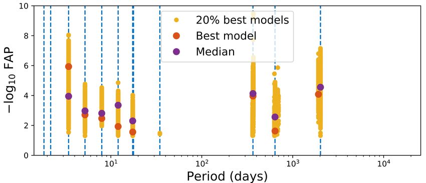
Fig. B.4. FAPs of the peaks of the 20% best models in terms of
Fig. B.1. `1 periodogram corresponding to the highest approximate evi- Laplace approximation of the evidence that have a FAP > 0.05. The
dence. periods marked in red in Fig. 2 are represented by the blue dashed
lines.
Histogram of cross validation scores
1200
Highest 20%
1000 Lowest 80%
800
Counts
600
400
200
0
550 500 450 400 350 300 250
Cross validation score
Fig. B.2. Histogram of the values of the cross validation score. Best
20% and lowest 80% are represented in blue and orange, respectively.
Fig. B.5. FAPs of the peaks of the 20% best models that have a FAP >
0.05, when adding a linear activity model fitted as a Gaussian process.
The periods marked in red in Fig. 2 are represented by the blue dashed
lines.
peaks selected are represented in Fig. B.3 by the yellow points.
For a comparison with the best models, that is, the model with
the maximal CV score, the periods appearing in the best model
(red dots in Fig. 2) are represented by the blue dashed lines. We
represent the median of the FAPs for each of these periods in the
CV20 and their FAP in the best models (purple and red, respec-
Fig. B.3. FAPs of the peaks of the 20% best models in terms of cross tively). These values are also listed in Table B.2, where we also
validation score that have a FAP >0.05. The periods marked in red in give the percentage of cases where a period corresponds to a FAP
Fig. 2 are represented by the blue dashed lines. < 0.05 in CV20 .
We plotted the same Fig. B.3 and the same Table B.2 for
the 20% best models in terms of evidence (E20 ) (Fig. B.4 and
model. As a result of this procedure, each noise model has a Table B.3). The `1 periodogram corresponding to the highest
cross validation score (CV score). ranked model is shown in Fig. B.1). Peaks at 3.4, 5.2, 7.9, and
The second metric is the approximation of the Bayesian 12 d have similar behaviors with cross validation and approxi-
evidence of the (noise model, planets) couple. For a given mate evidence. We see three notable differences when ranking
covariance matrix, we fit a sinusoidal model initialized at the a model with evidence: ≈10% of the selected models display
periods selected by the FAP criterion. We then made a second significant peaks at 1.84 or 2.17 d, 17.4 reaches a 5% FAP in
order Taylor expansion of the posterior (with priors set to one in only 38% of E20 , and 8% of the models favor 17.4 over 17.7 d.
all the variables) and estimated the evidence of the model, which Finally, the inclusion percentage and average FAP of long period
is also called the Laplace approximation (Kass & Raftery 1995). signals significantly drops. We have also ranked models with
The procedure is explained in greater detail in Nelson et al. AIC (Akaike 1974) and BIC (Schwarz 1978), which yield results
(2020), Appendix A.4. very similar to approximate evidence.
In Fig. B.2, we represent the histogram of the values of the When using a LASSO-type estimator (Tibshirani 1994), such
CV score for all the noise models considered. The models with as the `1 periodogram, for a fixed dictionary (here, a fixed noise
the 20% highest CV score are represented in blue, and they model), it is common practice to select the model with cross-
present similar values of the CV score. We call the set of these validation as the solution follows the so-called LASSO path.
models CV20 . Here, this would constitute a viable alternative to selecting the
Each model of CV20 might lead to different peaks selected peaks that have FAP < 0.05. This was tested on a grid of param-
with the FAP < 0.05 criterion. The periods and FAPs of the eters such as B.1, and it yields very similar conclusions.
L6, page 11 of 17A&A 636, L6 (2020)
HD 158259 logRhk, raw and smoothed Table B.3. Periods appearing in the `1 periodogram of the model
4.65
with the highest approximated evidence and their false alarm
Raw data probabilities.
4.70 Smooted data
4.75 GP prediction
Period (d) FAP (best fit) Inclusion in the model E20 median FAP
logRhk
4.80
1.839 1.00 0.714% –
4.85
2.178 1.83 × 10⁻³ 9.486% –
4.90 3.432 5.78 × 10⁻¹² 100.0% 1.98 × 10⁻⁸
4.95 5.197 7.49 × 10⁻⁸ 100.0% 1.23 × 10⁻⁵
7.953 8.67 × 10⁻⁷ 100.0% 3.15 × 10⁻⁵
56000 56500 57000 57500 58000 58500 12.03 1.38 × 10⁻⁴ 90.38% 4.35 × 10⁻³
Time (rjd) 17.4 1.00 38.07% –
Fig. B.6. Raw and smoothed log R0HK time series. The dark blue points 17.74 4.81 × 10⁻³ 8.771% –
represent the raw log R0HK data used for the prediction. The light blue 34.59 1.00 0.0% –
lines represent the Gaussian process prediction and its ±1σ error bars 365.7 1.00 56.07% –
(see Eq. (B.2)). The orange points are the predicted values of the Gaus- 640.0 1.00 8.966% –
sian process at the radial velocity measurement times. 1920. 1.00 39.44% –
Notes. Third columns: percentage of models in the 20% best evidence
Table B.2. Periods appearing in the `1 periodogram of the model with (E20 noise models) where the periodicity has a FAP < 0.05, and the
the highest CV score and their false alarm probabilities. fourth column shows the median FAP of these periodicities in the E20
models.
Period (d) FAP (best fit) Inclusion in the model CV20 median FAP
1.839 1.00 0.0% – B.3. Discussion
2.178 1.00 0.0% –
3.432 1.97 × 10⁻⁵ 100.0% 3.03 × 10⁻⁴ The noise model has a strong impact on the false alarm proba-
5.197 8.02 × 10⁻³ 100.0% 1.03 × 10⁻³ bilities. When instantiating the covariance matrix with an expo-
7.953 1.83 × 10⁻³ 100.0% 1.63 × 10⁻³ nential kernel, such as Eq. (B.2), the characteristic time τ can be
12.03 2.76 × 10⁻³ 100.0% 2.55 × 10⁻⁴ seen as setting the threshold between “short” and “long” peri-
17.4 2.26 × 10⁻² 100.0% 4.75 × 10⁻³ ods. The FAPs of the signals with periods lower than τ are lower
17.74 1.00 0.0% –
and higher, respectively, compared to the ones computed with a
34.59 1.00 0.0% –
365.7 1.11 × 10⁻⁶ 100.0% 2.17 × 10⁻⁷
white noise model. Using a correlated noise model reduces the
640.0 1.35 × 10⁻² 89.79% 1.39 × 10⁻³ chances of spurious detection claims at long periods, but on the
1920. 2.12 × 10⁻² 100.0% 8.15 × 10⁻⁴ other hand, it decreases the statistical power (see Delisle et al.
2020 for a more detailed discussion on that point). The proce-
Notes. The third columns show the percentage of models in the dure of Sect. B.1 aims to balance the two types of errors: If the
20% best CV score (CV20 noise models) where the periodicity has a white noise model cannot be excluded (here, this means being in
FAP < 0.05, and the fourth column shows the median FAP of these peri- the best 20% noise models), then the short and long period sig-
odocities in the CV20 models. nal appear with lower and higher FAPs, respectively, resulting in
a compromise value. We have found the result to be insensitive
B.2. Long-term model to the exact threshold on the models selected (choosing the best
10, 20, and 30% yields identical conclusions). The interpretation
It has been found that the log R0hk has a strong long-term signal. of the differences between cross validation and evidence is that
This one can be included in the analysis with a Gaussian process evidence appears to favor models with stronger correlated com-
analysis, similarly to Haywood et al. (2014). We consider a sim- ponents, which damp the amplitude of long period signals and
ple covariance model for the log R0HK boost high frequency signals.
(tk −tl )2
We have found that signals at 3.43, 5.19, 7.95, 12.0, 17.4, and
− 366 d consistently appear in the models. The 1920 and 640 d sig-
Vkl (θ) = δk,l σ2W + σ2C c(k, l) + σ2R e 2τ2
R . (B.2)
nals appearing in Sect. B.1 disappear when modeling the activ-
We assume that σR is equal to the standard deviation of ity as in Sect. B.2, pointing to a stellar origin. The strength of
the log R0HK data, and we fit the parameters σW and τ. We find the 17.4 d signal varies with the model ranking technique, which
σW = 0.9σR and τ = 770 d. We then predicted the Gaussian makes its detection less strong than the other signals. We, how-
process value and its covariance with formulae 2.23 and 2.24 ever, note that this one was put in competition with a quasi-
in Rasmussen & Williams (2005). In Fig. B.6, we represent the periodic model at the same period, which is not the case of the
raw log R0HK data on which the fitting is made. The Gaussian other signals. Overall, we claim that the 3.43, 5.19, 7.95, 12.0,
process and the one sigma standard deviation of the marginal 17.4, and 366 d periodicities are present in the signal and there
distribution at t are represented in light blue, and the prediction is a candidate at 1.84/2.17 d.
at the radial velocity measurement times is in orange. As a remark, the noise model selection procedure is close
We then performed the same analysis as in Sect. B.1, except to Jones et al. (2017), which ranks noise models with cross vali-
that we include the smoothed log R0HK (orange points in Fig. B.6) dation, BIC, and AIC. The difference lies in the fact that instead
as a linear predictor in the model. The results are presented in of comparing noise models with free parameters, we compare
Fig. B.5. These are almost identical to the results of Sect. B.1, models that are couples of the noise model with fixed parame-
except that the 2000 d and 640 d signals disappear. ters and planets with fixed periods.
L6, page 12 of 17You can also read