Where Is the Clean Air? A Bayesian Decision Framework for Personalised Cyclist Route Selection Using R-INLA
←
→
Page content transcription
If your browser does not render page correctly, please read the page content below
Bayesian Analysis (2021)                  16, Number 1, pp. 61–91

    Where Is the Clean Air? A Bayesian Decision
     Framework for Personalised Cyclist Route
              Selection Using R-INLA∗
Laura C. Dawkins† , Daniel B. Williamson†,‡ , Kerrie L. Mengersen§ , Lidia Morawska¶ ,
                     Rohan Jayaratne¶ , and Gavin Shaddick†,‡

      Abstract. Exposure to air pollution in the form of fine particulate matter (PM2.5 )
      is known to cause diseases and cancers. Consequently, the public are increasingly
      seeking health warnings associated with levels of PM2.5 using mobile phone ap-
      plications and websites. Often, these existing platforms provide one-size-fits-all
      guidance, not incorporating user specific personal preferences.
         This study demonstrates an innovative approach using Bayesian methods to
      support personalised decision making for air quality. We present a novel hierarchi-
      cal spatio-temporal model for city air quality that includes buildings as barriers
      and captures covariate information. Detailed high resolution PM2.5 data from
      a single mobile air quality sensor is used to train the model, which is fit using
      R-INLA to facilitate computation at operational timescales. A method for eliciting
      multi-attribute utility for individual journeys within a city is then given, providing
      the user with Bayes-optimal journey decision support. As a proof-of-concept, the
      methodology is demonstrated using a set of journeys and air quality data collected
      in Brisbane city centre, Australia.

1     Introduction
Air pollution is a major environmental risk to health, estimated to cause 4.2 million pre-
mature deaths worldwide annually (World Health Organization, Accessed: 27-11-2018),
and 3000 deaths each year in Australia (Australian Institute of Health and Welfare,
2016). Exposure to fine particulate matter (2.5 microns or less in diameter, abbreviated
to PM2.5 ) is known to causes cardiovascular and respiratory diseases, and cancers (Sava
and Carlsten 2012; Hoek et al. 2013; Loomis et al. 2013).
    The general public is becoming increasingly aware of the negative health impacts
associated with exposure to PM2.5 . As a consequence there is an increasing demand
for air quality information and warnings via online web-based tools and mobile phone

   ∗ This article was first posted without an Acknowledgements section. The Acknowledgements section

was added on 8 January 2020.
   † College of Engineering, Mathematics and Physical Sciences, University of Exeter, UK,

lauradawkins@hotmail.co.uk
   ‡ The Alan Turing Institute, British Library, London, UK
   § Science and Engineering Faculty, Queensland University of Technology, Australia
   ¶ International Laboratory for Air Quality and Health, Queensland University of Technology, Aus-

tralia


c 2021 International Society for Bayesian Analysis           https://doi.org/10.1214/19-BA1193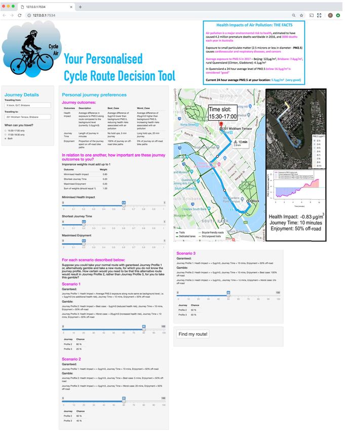
62 A Bayesian Decision Framework for Personalised Cycle Route Selection

applications. In most cases, these websites and applications provide generic, one-size-
fits-all air quality measurements or warnings for a given location, either based on a
single nearby air quality monitoring station, a numerical weather prediction model, or a
network of stationary monitoring stations used in combination with a dispersion model,
land use regression model and/or satellite data. Examples of such platforms include
the Queensland Government live hourly air quality data table (Queensland Govern-
ment, Accessed: 14/12/2018), Plume (Plume Labs, Accessed: 27-11-2018), BreezoMeter
(BreezoMeter, Accessed: 27-11-2018) and MappAir (MappAir, Accessed: 27-11-2018).
In many cases these air quality warning platforms provide associated health warnings,
often based on the national Air Quality Index (AQI) guidelines which indicates, for ex-
ample, when it is best to avoid certain activities outside. Again, however, these health
warnings are not specific to the user and no platforms consider other parameters of
importance, for example the inconvenience of avoiding highly polluted areas.
    Here we present a novel approach for combining Bayesian decision theory and hierar-
chical Bayesian spatio-temporal modelling to inform a personalised air quality warning
tool, able to provide Bayes-Optimal decision support about which route a given user
should take through a city.
    In order to develop a personalised decision making framework, a multiattribute util-
ity function must capture a user’s preferences over competing rewards (Smith, 2010). For
example, suppose two potential journeys exist from A to B, one characterising a highly
polluted, short route and an alternative characterising a cleaner, longer route. Suppose
a given individual is most concerned with arriving at their destination as quickly as
possible while another considers the impact on their health to be most important: the
optimal route for each individual is likely to be different. Here we present a method
for eliciting these complex preferences about competing journeys, and show how they
can be used to inform a Bayes-Optimal route for a given individual. Specifically, pref-
erences about three decision-relevant journey attributes are considered: a measure of
the health impact of exposure to PM2.5 along the journey, the journey time in minutes,
and a measure of the journey enjoyment. In a similar way, Economou et al. (2016) used
a Bayesian decision analysis approach within an environmental hazard application to
provide personalised meteorological natural hazard warnings for individual stakehold-
ers. Predominantly, however, such theory has not been utilised in this field. A detailed
description of Bayesian decision analysis can be found in Smith (2010). Here, as a proof-
of-concept, we focus on developing a Bayesian decision theoretic tool for personalised
cycle route selection in Brisbane city centre.
    In addition to capturing users preferences, we require a probability model for PM2.5
exposure for any route that a user may choose. To achieve this, we develop a Bayesian
hierarchical spatio-temporal model for PM2.5 , able to accurately predict PM2.5 exposure
along potential routes within the geographical domain. Stationary air quality monitor-
ing stations are limited in their spatial coverage and are therefore unable to represent
the spatial variability relevant for assessing personal exposure to pollution along a route.
Consequently, in recent years mobile air quality monitors have become increasingly used
as an additional tool to acquire air quality data at high spatial and temporal resolutions,
and at locations most relevant for personal exposure (Van den Bossche et al., 2015). This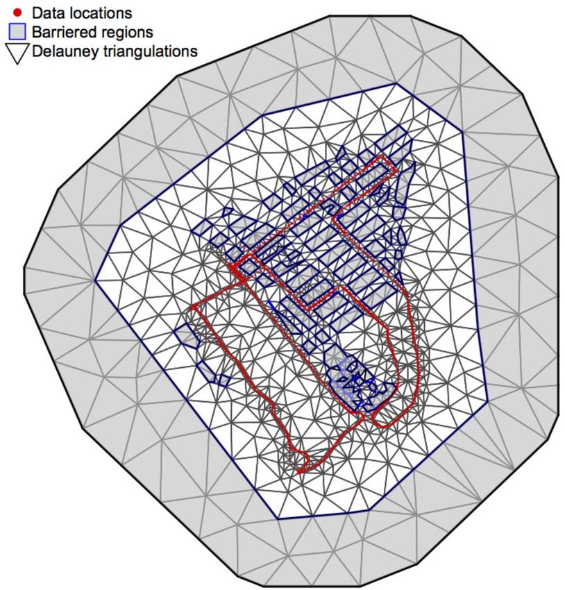
L. C. Dawkins et al.                                                                  63

increase in mobile air quality sensing comes after recent improvements in low cost mo-
bile monitors. These include the Airoflex monitor, used by Elen et al. (2013) to monitor
ultra fine particles (UFP) and black carbon (BC) in Antwerp, Belgium, and the KOALA
(Knowing Our Ambient Local Air-quality) monitor, recently developed by the Interna-
tional Laboratory of Air Quality and Health (ILAQH), Australia, used to monitor air
quality at the 2018 Commonwealth Games (ILAQH, Accessed: 28-11-2018). A compre-
hensive overview of the rapidly growing body of literature on mobile air quality sensing
can be found in Van den Bossche et al. (2015), in combination with Xie et al. (2017).
    Hierarchical Bayesian models provide a useful framework for representing complex
air quality data. A number of examples of such models exist for stationary air quality
monitoring stations, for example Cocchi et al. (2007), Sahu and Bakar (2012) and Li
et al. (2013). However more recently, in response to the growing recognition of mobile
air quality monitors, Del Sarto et al. (2016) developed a hierarchical Bayesian spatio-
temporal modelling approach for representing such data. This model uses a three level
hierarchy in which the mobile observations are modelled in the first stage of the hi-
erarchy, and a latent spatio-temporal process, defined on a discrete space-time grid,
is considered in the following stages, also capturing covariate information. As such,
this form of hierarchical Bayesian model is able to give a detailed representation of air
quality at the most relevant locations (i.e. where people actually travel), whilst also
providing a comprehensive quantification of uncertainty. This allows for more specific
and accurate personal guidance on where and when to go to minimise exposure to harm-
ful air pollution, compared to current air quality warning platforms. In addition, the
recent advancements in computational tools for implementing the Integrated Nested
Laplace Approximation (INLA) approach for Bayesian inference (Rue et al., 2009), a
computationally efficient alternative to Markov Chain Monte Carlo (MCMC) methods,
facilitates the application of such complex hierarchical Bayesian models at operational
timescales, for example to provide real-time air quality warnings. In addition, rather
than assuming a stationary spatial field our INLA air quality model incorporates an
adaptation of the barrier model of Bakka et al. (2018), originally developed to model
coastlines, to better represent the way in which high-rise buildings block the flow of air
within the city, causing non-stationarity.
    Following this we explore approaches for equating exposure to PM2.5 along a given
route to the associated impact on health, the first decision-relevant journey attribute.
The other two decision-relevant journey attributes, journey time and enjoyment, are
estimated using Google maps and Google route planner. We then present an approach
for eliciting the personal preferences of the user, including an R Shiny web interface.
    We present a proof-of-concept cycle route selection tool tailored to comparing two
alternative routes through Brisbane city centre, shown in Figure 1, at two different
times of the day. These routes have differing characteristics to demonstrate how distinct
personal preferences will result in a particular cycle route selection. Route 1 (purple)
is predominantly cycled next to the river along a scenic cycle path, reducing exposure
to PM2.5 , increasing journey enjoyment, but also increasing journey time, while route
2 (blue) is shorter and quicker but predominantly cycled on the busy roads within the
Central Business District (CBD), increasing exposure to PM2.5 and reducing journey
enjoyment.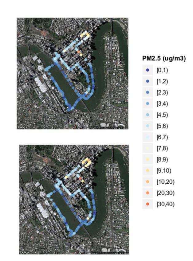
64 A Bayesian Decision Framework for Personalised Cycle Route Selection

Figure 1: A google map showing the two routes used within this proof-of-concept study
to demonstrate how our method optimises different journeys based on differing personal
preferences. These two routes go between X block at Queensland University of Technol-
ogy (QUT) and Wickham Terrace to the north of the Central Business District (CBD)
taking different cycle friendly paths.

    The remaining paper is organised as follows. In Section 2 we present our approach
to quantifying the decision-relevant attributes for our proof-of-concept application in
Brisbane, including a description of the mobile monitor data collection scheme in Sec-
tion 2.1, the development of the Bayesian spatio-temporal model for mobile air quality
monitor data using INLA in Section 2.2, and the subsequent representation of the three
decision-relevant journey attributes, in particular how PM2.5 exposure is related to
health in Section 2.3. Section 3 outlines the method for eliciting user-specific prefer-
ences for the Bayesian decision framework, followed by the case study demonstration of
the decision framework in Section 4. Finally Section 5 concludes.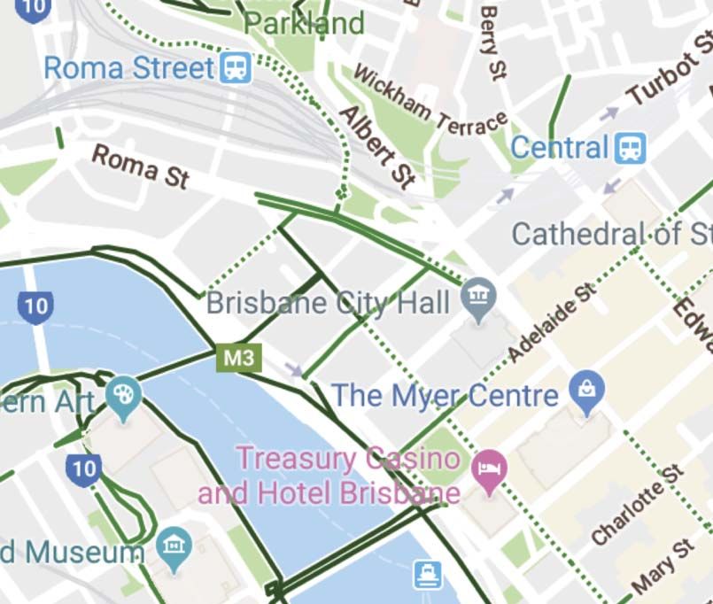
L. C. Dawkins et al.                                                                           65

2     Quantifying Decision-Relevant Journey Attributes
Let d represent the decision to choose a particular cycle route; θ represent the exposure
to PM2.5 along this chosen route; y denote all available relevant data; and r(d, θ) =
(r1 (d, θ), r2 (d, θ), r3 (d, θ)) represent the three decision-relevant journey attributes for the
chosen route: health impact of exposure to PM2.5 , journey time, and journey enjoyment
respectively. Bayesian decision theory shows that the optimal decision d∗ (y) is the one
that maximises the expected utility, which, if mutual independence between attributes
is assumed, can be written as:
                                          3

                               Ū (d) =         ki Ui (ri (d, θ)) p(θ|y)dθ,                    (1)
                                    θ   i=1

where Ui is a utility function, and ki the criterion weight for decision-relevant journey
attribute i. The criterion weight, ki , characterises how important the   decision maker
considers attribute i to be in relation to the other attributes, such that i ki = 1, while
the utility function, Ui , represents how risk adverse the decision maker is to incurring
a bad outcome of attribute i (see Smith (2010) and references there in for more detail).
The assumption of mutual independence is a made here to allow the paper to focus on
demonstrating the framework, however an alternative dependence structure could be
modelled using Bayesian decision theory. This is discussed further in Section 5.
    In Section 3 we develop a method for eliciting Ui and ki for i = 1, 2, 3 from the user.
Firstly, however, in this section we develop our probability model for θ (PM2.5 exposure),
including an efficient method for inference given mobile air quality monitor data, y.
Following this, an approach for relating exposure to PM2.5 to adverse health impacts
is developed, quantifying r1 . The other decision-relevant attributes, journey time and
journey enjoyment (r2 and r3 ), are obtained without requiring the development of a
statistical model. Journey time is manually extracted from Google Maps, while journey
enjoyment is calculated as the proportion of the journey time spent cycling off-road (i.e.
not on a section of the route within the CBD).

2.1    Data
The air quality data used within this application were collected using a compact, state-
of-the-art, portable air quality monitor (26 × 21 × 11 cm), KOALA (Knowing Our
Ambient Local Air-quality), developed by scientists at the International Laboratory of
Air Quality and Health (ILAQH) at Queensland University of Technology (QUT), in
Brisbane, Australia, as part of a larger project on establishing advanced networks of
air quality sensing and analysis (ILAQH, Accessed: 28-11-2018). The KOALA monitor
includes two low-cost sensors that measure PM2.5 and carbon monoxide concentrations
in real time. Readings were obtained at 5-second intervals and stored on a built-in SD
card for later download and analysis.
  For this study the monitor was attached to the front basket of a bicycle and used
measure PM2.5 concentration along roads and cycle paths within Brisbane city centre.
A GPS tracker was attached to the bike alongside the KOALA monitor, recording its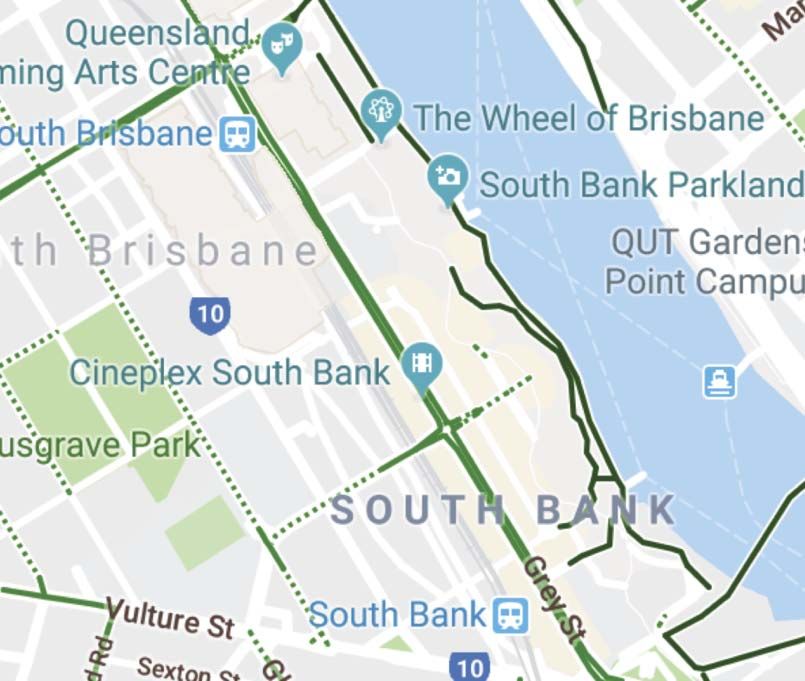
66 A Bayesian Decision Framework for Personalised Cycle Route Selection

location at approximately equivalent time intervals. In this way the mobile monitor was
able to provide data at a high spatial resolution, in locations relevant for presenting
personal exposure to PM2.5 while cycling through the city centre.
   The high temporal variability of urban air quality means that achieving a repre-
sentative data sample requires careful consideration of three factors: the geographical
location of the data collection route, the most relevant times at which to collect the
data (i.e. which days of the week and times of the day?), and the frequency of repeated
data collection laps.
    Primarily, since this study is focused on developing a tool for cyclists and the data
was to be collected on-bike, the data collection route was restricted to “cycle friendly”
routes only, as defined by Google Maps. In addition, the physical exertion involved in
collecting the data restricted the route to an approximately 2 km2 central region of Bris-
bane city (longitude range 153.0193:153.0316, and latitude range −27.48214:−27.46464).
As in previous similar studies using mobile air quality monitors such as Van den Boss-
che et al. (2015) and Peters et al. (2013), the route was designed to encompass the
varying terrain and road types within the city centre. Specifically here, this meant en-
suring the route included the on-road bike paths within the Central Business District
(CBD); the pedestrianised routes through the Botanic Gardens, situated to the south
of the CBD; the Bicentennial bike-way running along the Brisbane river to the west of
the CBD; and the pedestrianised route on the other side of the river, known as South
Bank. In addition, the route was devised to encompass the most popular cycle routes
within these four regions, based on the freely available STRAVA (social fitness network)
heat map, a visualisation of the frequency with which roads are used by their cyclist
subscribers (Strava, Accessed: 14-01-2019). Finally, the route was designed to include
likely destinations for cyclists journeying into the city centre, namely bicycle parking
racks and the bike stations of the local bike sharing scheme, CityCycle. The final route,
as shown in Figure 2, was approximately 8 km in length, taking roughly 35 minutes to
complete.
   The temporal data collection schedule was designed to capture the days of the week
and times of the day most frequented by cyclist. Mateo-Babiano et al. (2016) presented
an analysis of the CityCycle usage habits of people living and working in Brisbane
between May 2012 and April 2013. Mateo-Babiano et al. (2016) identified a general
peak in CityCycle usage on weekdays during the morning commute 6:00–10:00, and the
evening commute 16:00–19:00, and on weekends during the middle of the day 10:00–
16:00. Similarly, as an ongoing initiative to improve cycling infrastructure in Brisbane
the city council have been carrying out cyclist counts throughout the city, published
by the Brisbane Times, identifying the same peaks in cyclist numbers (Brisbane Times,
Accessed: 14-01-2019). They provide specific counts for Brisbane CBD (separate from
other regions of the city), indicating a slightly later peak in the morning commute (6:30–
10:30) and a slightly earlier peak in the evening commute (15:30–18:30), capturing how
the CBD is the most common place of work and is therefore the end point of morning
commute and start point of the evening commute. In addition, this count revealed that
Tuesdays and Thursdays have slightly higher cyclist numbers than other weekdays, and
Sundays are marginally more popular with cyclists than Saturday.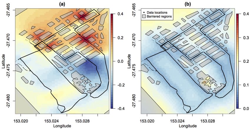
L. C. Dawkins et al.                                                                   67

Figure 2: (a) The cycle route devised for data collection, indicating the different regions
of Brisbane city centre (CBD, bike-way, South Bank and Botanic Gardens) and the
location of bike racks and CityCycle docking stations, (b) The STRAVA heat map for
Brisbane city centre.

    The data collection schedule on a given day was restricted by the battery life and
charging time needed for the KOALA monitor to operate. Once fully charged the mon-
itor could run for 3 hours at a time and then required another 4 hours to charge in
between runs. Following this restriction and the peak cycling times identified by Mateo-
Babiano et al. (2016) and Brisbane City Council, the data collection on weekdays was
organised into 4 time slots: one early morning commute (7:00–8:30), one later morning
commute (8:30–10:00), one early evening commute (15:30–17:00) and one later evening
commute (17:00–18:30). Data collection on the weekend was organised into 2 time slots:
early leisure time (10:00–11:30) and later leisure time (11:30–13:00).
    Finally, the required number of repeated data collection laps was considered. As
identified by Van den Bossche et al. (2015) and Peters et al. (2013), high resolution spa-
tial mapping of air quality requires repeated mobile monitor measurements. Peters et al.
(2013) concluded that a limited set of mobile measurements (20–24, and for some streets
as few as 10) made it possible to map air quality, while Van den Bossche et al. (2015)
identified that, depending on the location, 24–94 (median 41) repeated measurements
were required. Here, data collection was carried out by a team of 16 volunteers, restrict-
ing the availability of participation, within a limited project time frame. Following the
Brisbane cycle count results, data collection was allocated to Tuesday, Thursday and
68 A Bayesian Decision Framework for Personalised Cycle Route Selection
Sunday during a short period of 2 weeks running from Thursday 10th May–Thursday
24th May 2018, encompassing 2 Tuesdays, 3 Thursdays and 2 Sundays, hence 7 days in
total. To increase the number of repeated laps and hence the representativeness of the
sample, the route was completed twice within each of the time slots on each of the data
collection days. This resulted in a total of 48 laps of the data collection route, within
24 time slots, over 7 days within a 2 week period in May 2018, made up of a total of
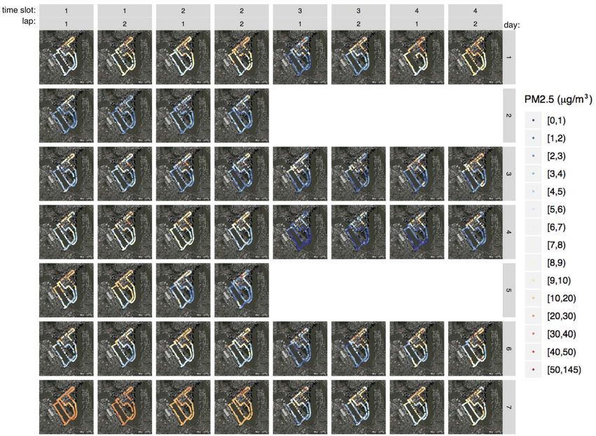
15847 data points. These 48 laps are shown in Figure 3. Following data collection, to
ensure PM2.5 was recorded along cycle routes, ArcGIS was used to move GPS locations
associated with each data point to the nearest location along the route.
Figure 3: The 48 PM2.5 laps of data collected using the KOALA mobile air qual-
ity monitor. These 48 laps were collected over 24 time slots, (1–4) on weekdays and
(1–2) on weekends [columns], and 7 days in May 2018 (Thursday 10/05/2018, Sunday
13/05/2018, Tuesday 15/05/2018, Thursday 17/05/2018, Sunday 20/05/2018, Tuesday
22/05/2018, Thursday 24/05/2018) [rows].
Further data used within this study consisted of 5 minute average PM2.5
concentrations and hourly average meteorological measurements (temperature, wind
direction, wind speed and humidity) from three stationary monitoring stations lo-
cated in Wooloongabba, South Brisbane and the Queensland University of Technol-
ogy campus, available from the Queensland Government (Queensland Government,
L. C. Dawkins et al.                                                                           69

Accessed: 14/12/2018). In addition, electronic 30 minute total traffic counts at four
intersections within the city centre (Adelaide Street – Wharf Street, Elizabeth Street –
George Street, Elizabeth Street – Edward Street and Mary Street – Albert Street) were
kindly provided by Brisbane City Council. For each variable described above the avail-
able data was used to calculate an average for each of the 1.5 hour time slots within
the data collection schedule. Finally, geographical variables akin to those used in air
quality land use regression models (e.g. Hoek et al., 2008) were derived using ArcMap,
including, for each data point, the distance from a major junction and distance from
the river. The junctions considered ‘major’ were those at which the cyclists were often
made to wait at traffic lights for a long period of time, shown in Figure 2.

2.2      A Spatio-temporal Model for Mobile Air Quality Monitor Data
         Using the INLA Barrier Model
We develop a spatial-temporal model for mobile air quality data, building upon the
model presented by Del Sarto et al. (2016). We consider a model structure in which
realisations of the spatial-temporal process are indexed by a nested time structure and
spatial grid. That is, for day d = 1, . . . , D, time slot t = 1, . . . , Td and spatial grid cell
s = 1, . . . , S, Zdts represents the spatial process at the spatio-temporal point dts. As the
mobile data collection route is completed, multiple observations are made within the
vicinity, and hence are representative of each of these spatio-temporal points. Therefore,
let Ydtsj for j = 1, . . . , Jdts represent these Jdts repeated observations at the spatio-
temporal point dts. The mobile data collection routes vary slightly each time they are
completed, hence Jdts can be different for each grid point dts. Similar to Del Sarto
et al. (2016), we model this data using a Hierarchical Bayesian framework, in which
each nested index is modelled as a different layer of the hierarchy. This allows us to
incorporate covariates at each level of the model and to model different sources of
error separately. Let the mobile air quality monitor observations be denoted Yi , for
i = 1, . . . , dtsj, . . . , N (where N = DTD SJDTD S ), then,

                                     Yi = μi + ei ,                                          (2a)
                           μi = μdtsj = Zdts + β0 + βXdtsj + ξdtsj ,                         (2b)
                                  Zdts = Zdt + β̃ X̃dts + dts ,                             (2c)
                                   Zdt = Zd + φdt ,                                          (2d)

                                    Zd = Z + β         Xd   + ψd ,                          (2e)
                                     Z ∼ GF (0, Σ),                                          (2f)

where:

   • Yi is the ith observation, i = 1, . . . , dtsj, . . . , N ,

   • μi is the mean, and ei the error, associated with observation i,

   • Zdts is the latent process at spatio-temporal grid point dts,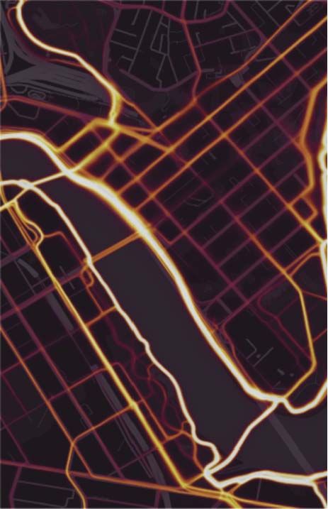
70 A Bayesian Decision Framework for Personalised Cycle Route Selection

   • β0 is the overall intercept coefficient, constant for all observations,

   • Xdtsj is a p × 1 vector of covariates available for each observation,

   • β is the p × 1 vector of coefficients associated with these p covariates,

   • ξdtsj is the error within spatial locations, for example in our data accounting for
     the difference in the two laps of the data collection route within each time slot,

   • Zdt is the latent process at time dt,

   • X̃dts is a p̃ × 1 vector of covariates available on the same resolution as the spatio-
     temporal points dts only,

   • β̃ is the p̃ × 1 vector of coefficients associated with these p̃ covariates,

   • dts is the error among spatial locations,

   • Zd is the latent process on day d,

   • φdt is the error among time slots,

   • Z is a zero mean non-stationary Gaussian random field with spatial covariance
     matrix Σ, defined over the spatial field s = 1, . . . , S,

   • Xd is a p × 1 vector of covariates available for each day only,

   • β  is the p × 1 vector of coefficients associated with these p covariates,

   • ψd is the error among days.

    This model differs from that of Del Sarto et al. (2016) in a number of ways. An
additional level is added to the top of the hierarchy such that each observation has an
associated error term. This additional error term is necessitated by the repeated lap
structure of the data collection route, which results in data points recorded approxi-
mately an hour apart being considered to be at the same spatio-temporal grid point. In
addition, the auto-regressive (AR) temporal component of the Del Sarto et al. (2016)
model is omitted from this model structure. Again, this is due to the differing temporal
structure of our data. Del Sarto et al. (2016) consider hourly data throughout a number
of consecutive days, while here, we consider two/four disjointed 1.5 hour time slots dur-
ing non-consecutive weekends/weekdays. Further, we include an additional level at the
bottom of the hierarchy to capture the variability between days, in terms of covariates
available for each day only and the error among days.
    Moreover, rather than using MCMC as in Del Sarto et al. (2016), here the Gaus-
sian random field (GF) Z(s) is modelled using a computationally efficient alternative to
MCMC, the Integrated Nested Laplace Approximation (INLA), Stochastic Partial Dif-
ferential Equation (SPDE) approach of Lindgren and Rue (2011). The advantage of this
approach, compared to using an MCMC approach, is its applicability to very high di-
mensional data and reduced computational time and expense. This facilitates Bayesian
L. C. Dawkins et al. 71
model fitting in real time, as would be required for making air quality predictions within
a web or mobile phone application.
Finally, unlike the model of Del Sarto et al. (2016), the non-stationarity of the spatial
domain resulting from topographical variability of multi-storey high-rise buildings, is
captured by using the non-stationary barrier model extension of the INLA framework,
originally developed by Bakka et al. (2019) to model coast lines. A physical barrier is
specified, and the solutions to the SPDEs representing the barriered and non-barriered
regions, as specified in Bakka et al. (2019), are obtained. As in the stationary INLA
model, this is achieved by approximating the SPDE solution using a finite element
method, whose elements are vertices of Delauney triangulations over the spatial domain
(Shaddick and Zidek, 2014). A full description of the INLA SPDE approach can be
found in Lindgren and Rue (2011), and a useful summary is given by Shaddick and
Zidek (2014). The barrier model is specified in full in Bakka et al. (2018) and can
be implemented using the R-INLA R package, instructions and examples of which are
available within comprehensive tutorials at http://www.R-INLA.org/.
Modelling PM2.5 in Brisbane City Centre
Here, we model PM2.5 in Brisbane city centre, over the data collection schedule discussed
in Section 2.1. Similar to many examples in the literature including Del Sarto et al.
(2016), we model the log transformation of PM2.5 , which has been shown to be well
represented by the Normal distribution. In addition, we apply this log transform to
PM2.5 + 1 to ensure non-infinite transformed values.
Based on our previous Brisbane air pollution work (e.g. Morawska et al. 2002), other
relevant literature, and available relevant data (described in Section 2.1), we conducted
a preliminary exploratory data analysis to identify relevant covariate information to in-
clude within the different levels of our Bayesian Hierarchical model (2). This exploration
involved both the study of scatter plots of possible relevant relationships within the data,
and model comparison using the Watanabe-Akaike Information Criterion (WAIC), as
recommended by Gelman et al. (2014) and included within the R-INLA package, re-
moving and including each covariate to explore all relevant combinations. Future work
could involve incorporating model selection within the model fitting using, for example,
shrinkage priors on the regression coefficient parameters. This is, however, beyond the
scope of this study.
Exploration of covariates associated with each observation, Xdtsj (2b), included ge-
ographical measures: distance to the nearest major junction (see Figure 2) and distance
to the river, obtained using ArcMap, and 30 minute resolution traffic counts at 4 major
intersections. The interaction between traffic counts and a factor representing the time
of day (i.e. which time slot) was included in the exploration to characterise how traffic
flows in and out of the city along different roads.
Relevant covariates available on the resolution of the imposed spatio-temporal grid,
Xdts (2c) included the background level of PM2.5 , represented by the level at the nearest
stationary monitoring station located in South Brisbane, and meteorological conditions
within the time slot. In a previous study of Brisbane air quality, Morawska et al. (2002)72 A Bayesian Decision Framework for Personalised Cycle Route Selection
identified a notable diurnal cycle in wind direction in Brisbane city centre, owing to its
geographical location (coastline close by to the east). In the morning the winds gener-
ally come from the west, blowing polluted air from the motorway onto the CBD, while
in the afternoons, the sea breeze from the east blows this polluted air away from the
CBD. Wind direction as a factor characterising wind from the east/west was therefore
included in the exploratory data analysis. In addition, the influence of boundary layer
height, often determined from temperature, humidity and wind speed, on air pollu-
tion concentration is well documented (Zhang et al., 2014; Kumar Mehta et al., 2017).
During morning rush hour, which is just after sunrise and hence during relatively cool
conditions, the vehicle emissions mix into a shallow boundary layer, thus increasing
pollution. As the day warms up, the boundary layer height increases so emissions are
mixed into a larger volume of air. Thus the effects of evening commuter emissions are
not as severe as the effects of morning commuter emissions; this can be seen in Figure 3.
To represent this phenomenon, temperature, humidity and wind speed were included in
the model exploratory analysis. Based on insights from previous work, it was expected
that the effect of meteorological parameters would be less pronounced within the CBD,
where roads are shielded by buildings. Following this insight, the interaction between
meteorological variables and a location factor (in CBD/not in CBD) were also included
in the exploration. Finally, a factor characterising the ‘day type’, as either weekday or
weekend was explored as a covariate available at the day level, Xd (2e).
After conducting the exploratory data analysis, the resulting covariates included in
the model are as follows (with hierarchy within the model shown in square brackets):
• Distance from a major junction (2b)
• Distance from the river (2b)
• Electronic traffic counts at 4 intersections in Brisbane CBD and the interaction
between these and the categorical variable for time of day (time slots 1–4) (2b)
• Average PM2.5 at the South Brisbane monitoring station during the proceeding
1.5 hours (2c)
• Meteorological variables and the interaction between these and the CBD binary
variable (0 = not in CBD, 1 = in CBD) (2c)
– Temperature at the Brisbane CBD monitoring station
– Wind Direction at the Brisbane CBD monitoring station, as a binary variable
(0 = East, 1 = West)
– Wind speed at the South Brisbane monitoring station
– Humidity at the South Brisbane monitoring station
• Day type, as a binary variable (0 = weekday, 1 = weekend) (2e)
The regression coefficients (β0 , β, β̃, β ) are each assigned a Normal prior (Gelman
et al., 2008). Where the exploratory data analysis indicated a clear negative or positiveL. C. Dawkins et al. 73
relationship between log(PM2.5 + 1) and the covariate, the corresponding prior mean
for that regression coefficient is set to −1 or 1 respectively, such that:
β0 ∼ N (0, 0.001-1 ),
βk ∼ N (ck , 0.001-1 ) for k=1,. . . ,p,
β̃k̃ ∼ N (c̃k̃ , 0.001 ) -1
for k̃ = 1, . . . , p̃,
βk ∼ N (ck , 0.001-1 ) for k = 1, . . . , p ,
where ck = (−1, 1, 1, 1, 1, 1), for distance to major junction, distance to river and all
four traffic counts respectively, c̃k̃ = (1, −1, 1, −1, 1), for PM2.5 at South Brisbane in
the preceding 1.5 hours, temperature, wind direction from the west, wind speed and
humidity respectively, and ck = 1, associated with the weekday day type factor. All
other prior means are set at zero. In all cases, the prior precision (inverse variance) is
set to 0.001 (the INLA default). Alternative precision parameters (0.01 and 0.1) were
explored for sensitivity, resulting in indistinguishable posterior distributions for the
model parameters (shown in the table given in the Supplementary Material (Dawkins
et al., 2020)).
A zero mean normal prior is assigned to each of the error terms in the model. The
precision of each of these priors is assigned a log-gamma hyper prior with shape and
rate parameters a and b, respectively.
ei ∼ N (0, σe2 ) 1/σe ∼ log-gamma(a, b),
ξdtsj ∼ N (0, σξ2 ) 1/σξ ∼ log-gamma(a, b),
dts ∼ N (0, σ2 ) 1/σ ∼ log-gamma(a, b),
φdt ∼ N (0, σφ2 ) 1/σφ ∼ log-gamma(a, b),
ψd ∼ N (0, σψ2 ) 1/σψ ∼ log-gamma(a, b).
As described in the R-INLA multilevel model tutorial (Faraway, Accessed: 13/12/2018),
the variance of each of these random effects is expected to be lower than the variance of
the residuals of the fixed-effects only model. Based on the exploratory data analysis this
variance is expected to be approximately equal to 0.2. These hyper prior parameters
are therefore chosen such that the mean of the log-gamma distribution of the precision
( ab ) 0.2, hence a = 0.5 and b = 0.1. Alternative combinations of these parameters were
explored (e.g. a = 1, b = 0.2), again making a negligible difference to the resulting
model inference.
Model Fitting
Fitting the INLA barrier model using R-INLA first requires the creation of a mesh of
Delauney triangulations, including the specification of a maximum triangle edge length,
a model domain boundary and the location of barriers within the domain. Within
this study the maximum triangle edge length was specified as 0.2 km within the inner
domain and 0.4 km in the outer domain, the boundary of the domain was constructed74 A Bayesian Decision Framework for Personalised Cycle Route Selection
as a polygon encompassing Brisbane city centre, and the barriers were specified as the
location of high-rise buildings within the domain. The resulting mesh created using
R-INLA is presented in Figure 4, consisting of 1090 triangle vertices.
Figure 4: Mesh of Delauney triangulations created using R-INLA to represent Brisbane
city centre within the spatial INLA barrier model for PM2.5 in Brisbane city centre.
Using this mesh in combination with the PM2.5 mobile monitor data, covariate
data, the model formula specified in (2) and priors specified above, model fitting takes
approximately 15 minutes with R-INLA.
The mean and 90% credible interval for each of the model parameters is summarised
in a table given in the Supplementary Material. The mean and standard deviation of
the INLA barrier model Gaussian random field (GF), Z in (2f), is presented in Figure 5.
The mean of the GF (Figure 5a) clearly shows how the barriers within the model affect
the spatial dependence in the domain, creating the non-stationary structure that would
be produced by high-rise buildings. The areas of peak mean pollution are at locations
on the busy roads within the CBD and the barriers create a more physically realistic
dependence structure in which high levels of background PM2.5 are funnelled down the
urban canyon created by the high-rise buildings. In addition, as would be expected,
the lowest levels of background PM2.5 are found in the botanic gardens, and similarly
the barriers within the model characterise how the high rise buildings might affect the
spatial dependence between the gardens and the nearby roads.
Figure 6 demonstrates how the model represents the observations included within
the model fitting. Figure 6 (a) indicates that there is close agreement between true andL. C. Dawkins et al. 75 Figure 5: (a) The mean, and (b) standard deviation, of the INLA barrier model Gaussian random field for PM2.5 in Brisbane city centre. Figure 6: (a) Scatter plot comparing posterior predictive mean (black points) and 90% prediction interval (black line) with true log(PM2.5 +1) for all mobile air quality monitor observations, and a comparison of (b) the posterior predictive mean and (c) true PM2.5 for one randomly selected lap (Tuesday 15th May 2018, lap 2 in the 8:30–10:00am time slot). predicted values up to high magnitudes of approximately log(PM2.5 + 1) = 3.8, equiva- lent to PM2.5 = 46 μg/m3 . The model is less able to represent extreme observed levels of PM2.5 . This underestimation is also observable in Figure 6 (b) and (c), where the peak
76 A Bayesian Decision Framework for Personalised Cycle Route Selection

observed PM2.5 in this lap, equal to 34 μg/m3 , is associated with a posterior predictive
mean of 25 μg/m3 and a predictive distribution 95% upper quantile of 33 μg/m3 . Ex-
amination of video footage of the data collection laps revealed that these extreme levels
of observed PM2.5 are often associated with being located behind large diesel vehicles,
such as busses, within the CBD. To improve the representation of such observations in
future model advancements, the location and movement of busses within the city cen-
tre could be modelled using bus timetable information, and by differentiating between
different vehicle types in the traffic counts, discussed further in Section 5. The R code
and data required to fit the model in this paper is given in the Supplementary Material.

Model Validation

The results of a 10-fold cross validation of the model are presented in Figure 7, in which
10 sub samples of the data are created and recursively retained from the model for
validation. In Figure 7, the true log(PM2.5 + 1) lies within the 90% prediction interval

Figure 7: Scatter plots comparing the posterior predictive mean (black points) and 90%
prediction interval (black line) with true log(PM2.5 + 1) for observations in each of the
ten 10-fold cross validation sub samples.

for 90.7, 90.0, 90.7, 91.1, 90.0, 92.1, 90.1, 90.6, 91.5 and 91.2% of the observations within
the validation sub sample for each of the ten plots repectively, indicating an adequate
level of predictability. As identified in Figure 6, again Figure 7 shows that the model is
less successful at representing higher values of log(PM2.5 + 1) > 3.5.

2.3    Relating PM2.5 Exposure to Adverse Health Effects
Communicating the risks associated with exposure to PM2.5 to the public is made most
effective by relating exposure to adverse health effects. For this reason many of the
existing air quality mobile phone applications and websites provide health warnings
L. C. Dawkins et al.                                                                    77

associated with the given air pollution measurement or forecast. These health warn-
ings are typically based on air quality indices, calculated as the ratio of the pollution
concentration and a government specified objective value. The index falls into one of
five categories: Very good (0–33), Good (34–66), Fair (67–99), Poor (100–149) and Very
poor (≥150), each with associated health warnings based on numerous health studies
and relevant research (Queensland Government, Accessed: 14/12/2018). For PM2.5 this
government standard is based on a 24 hour moving average of the concentration recorded
at that location. This approach is therefore useful when providing health warnings to
an individual located in roughly the same place for 24 hours, but not as relevant when
communicating the health impacts associated with instantaneous or short term changes
in exposure to PM2.5 , for example during a short cycle route moving from A to B.
    A recent study by the U.S. Environmental Protection Agency (Mannshardt et al.,
2017) aimed to translate the air quality index thresholds, and the associated health
warnings for the 24 hour PM2.5 standard guidelines, to those based on instantaneous
air quality information. This was achieved through quantile matching of the empirical
distribution of instantaneous air quality and the contemporaneous 24 hour moving av-
erage air quality. This approach, however, cannot be utilised in our study as it requires
large quantities (e.g. multiple days) of continuous air quality data recorded while cycling
the data collection route to adequately represent this relationship, data that was not
feasible to collect here. In addition, we argue that discretising PM2.5 exposure, available
on a continuous scale, using air quality index thresholds loses a great deal of detailed
exposure information when describing a specific cycle route.
    Alternative approaches, that do not discretise PM2.5 exposure, involve calculating
the change in the relative risk (RR) of dying from a respiratory disease as a result of a
given exposure to a pollutant. In medical research, the RR is calculated as the proba-
bility of mortality in the exposed group divided by the probability of mortality in the
unexposed group, based on large cohorts of participants, for different levels of exposure.
For example, based on numerous key studies, Pope et al. (2011) used a nonlinear power
function, fit to estimates of the relative risk of lung cancer mortality, cardiovascular
and cardiopulmonary mortality at differing life-time daily exposures to PM2.5 , to obtain
functions for calculating these relative risks from daily PM2.5 dosage. The resulting equa-
tions were defined as: RR(lung cancer mortality) = 1+0.3195×(daily PM2.5 dose)0.7433 ,
and RR(cardiovascular disease mortality) = 1 + 0.2685 × (daily PM2.5 dose)0.2730 .
     In both equations the PM2.5 dose is measured in mg/m3 = 1000 μg/m3 , hence, cy-
cling a short route through Brisbane city centre from A to B, resulting in typically no
more than an increase of 0.014 μg/m3 = 0.000014 mg/m3 when averaged over 24 hours,
gives a 0.0079% and 1.27% increase in risk of mortality from lung cancer and cardio-
vascular disease respectively. These equations, however, represent the RR based on this
change in daily PM2.5 dosage being experienced every day throughout an individual’s
life. Hence, this approach is not relevant for communicating the health risk specifically
associated with taking a given cycle route as a one off. In many cases, however, a cyclist
will take the same route a number of times in a week, something that could be learnt
through repeated use of the cycle route decision tool. In these cases, therefore, such a
RR health measure may be relevant in quantifying the health impact of this accumu-
lated additional exposure to PM2.5 over a life-time, as even a 1% increase in mortality
78 A Bayesian Decision Framework for Personalised Cycle Route Selection
risk will have an important impact on an individual’s health. Further, the number of
people affected within a population makes this a large scale and important issue.
An alternative approach for communicating the health risk from PM2.5 exposure is
to associate PM2.5 dosage with the equivalent number of cigarettes smoked. Pope et al.
(2011) identified that, based on the quantity of tar (a source of PM2.5 ) within a cigarette
as reported by National Cancer Institute (2001), a single cigarette contains an average
inhaled dose of 12 mg of PM2.5 . Therefore, using the example above, this cycle route is
equivalent to 0.0168% of a cigarette. Therefore, this is a very small number that may
not be useful for communicating the health risks associated with a short cycle route.
Hence, none of the aforementioned approaches are directly relevant for communicating
the health risk associated with a taking a short cycle route from A to B, as required
within this study. Indeed, these approaches are all related to long term effects, and
little data is available on short term effects resulting from short exposures to very high
concentrations. This highlights the importance of further research to understand the
health impact of instantaneous and short term exposures to PM2.5 .
For this exercise, therefore, an alternative, simple approach is taken. Firstly, the
route selection tool informs the individual of the risks associated with exposure to PM2.5
using a series of facts and figures relevant for their location. Examples of such health
impact facts and figures, relevant for Brisbane and consistent with the information
provided by Queensland Government (Queensland Government, Accessed: 14/12/2018)
are shown in the top right corner of Figure 9. Secondly, the tool provides a measure
of the average difference between the background 24 hour average PM2.5 concentration
in their location, and their exposure to PM2.5 along a given journey. That is for given
journey m, the health impact measure, Hm , is:
Hm = (Em (t) − G)dt, (3)
t
where Em (t) is PM2.5 exposure at time t for journey m, and G is the background 24
hour average PM2.5 level calculated from the nearest stationary air quality monitoring
station. Here, this integral is approximated by summing over predicted PM2.5 from the
spatio-temporal INLA barrier model at 5 second intervals, inline with the temporal
resolution of the observation data used to train the model.
This measure quantifies how taking a certain route effects an individual’s personal
exposure to PM2.5 within that journey period. This change in PM2.5 exposure can then
be related to health impacts using the facts and figures provided, and can be used to
consistently compare the health impacts of travelling via different routes and at different
times of the day within the Bayesian decision framework. It should be noted that this
measure has the potential to be negative, indicating improved health, since cycling in a
park or along a river is likely to relate to PM2.5 exposures lower than the background
average level.
Figure 8 presents an example of predicted health impact of two different journeys,
both based on taking route 1 in Figure 1 on Friday 25th May 2018, but at different
times: one in the afternoon time slot (15:30–17:00), journey A (left column), and oneL. C. Dawkins et al. 79 Figure 8: Graphical representation of the health impact of travelling through Brisbane city centre on Friday 25th May 2018 via route 1 in Figure 1, during two different time slots: (a) and (c) Journey A – the afternoon time slot (15:30–17:00), and (b) and (d) Journey B – and the evening time slot (17:00–18:30). Figures (a) and (b) show how the posterior predicted mean exposure to PM2.5 varies at 5 second intervals along journeys A and B respectively. Figures (c) and (d) show histograms of health impact calculated over the full posterior predictive distribution of PM2.5 for journeys A and B respectively. The corresponding health impact associated with the posterior mean exposure (top row) is represented by the pink line in histograms (bottom row). in the evening time slot, journey B (right column). During journey A traffic counts are lower and weather conditions favour better air quality, leading to lower predicted PM2.5 along this journey compared to journey B. As a result, the mean exposure to PM2.5 along journey A compared to background level (G = 5.5) leads to a negative health impact value, HA = −0.83, indicating a reduced health impact compared to inhaling the background level of PM2.5 , while for journey B, HB = 0.14, indicating an increased health impact compared to inhaling the background level of PM2.5 . Within the Bayesian decision framework, the full posterior predictive distribution for PM2.5 is used within (1) to calculate a distribution of health impacts for each journey (r1 (d, θ)). This ensures the optimal decision is made based on a comprehensive quantification of uncertainty. Figure 8 (c) and (d) show these health impact posterior predictive distributions for journeys A and B respectively. These posterior distributions are wide, both over lapping zero. However, exploration of the QQ-plots of these posterior distributions and for other pairs of journeys identifies a linear relationship, indicating that routes with larger health
80 A Bayesian Decision Framework for Personalised Cycle Route Selection

impacts based on the posterior predictive mean PM2.5 will also have the highest health
impact when integrated over the full distribution. Approaches for reducing this posterior
spread are discussed further in Section 5.

3    Eliciting the Utility Function
Referring back to (1), thus far in our Bayesian decision framework for cycle route se-
lection we have a method for estimating the state of nature θ, i.e. PM2.5 exposure
along the route, from available observations of PM2.5 , y; a representation of all possible
decisions, d, in the form of cycle routes from origin to destination; and an approach
for representing the decision-relevant outcomes, r1 (d, θ), the health impact of exposure
to PM2.5 along a given route, and r2 (d, θ) and r3 (d, θ), representations of the jour-
ney time and journey enjoyment. The remaining elements required from the framework
are the multiattribute utility function, U , and the criterion weights, k, which must be
elicited from the decision maker to represent their relevant personal preferences about
the decision-relevant attributes.
    In this study the aim is to develop a cycle route selection tool that could be used
by any member of the general public within a smart phone application or web page.
For practicality, the utility function must therefore be elicited based on only a limited
series of questions, using clear, non-technical language, and visualisations to ensure
understanding.
   Figure 9 presents a screen shot of an RStudio Shiny web application (RStudio, Inc,
Accessed: 18-12-2018), created to demonstrate how this might be achieved (associated
R code is available in the Supplementary Material). Going from left to right, the user
(decision maker) initially enters the cycle journey details: where they are travelling from
and to, and how flexible they are in their time of travel. Following this the personal
journey preferences are elicited.
    In Bayesian Decision Theory, most commonly the utility function for a given at-
tribute i, is elicited from the decision maker via a series of questions associated with a
set of ‘gambles’ (Smith, 2010). Initially the best and worst case scenarios of the rele-
vant attribute are defined, denoted r∗ and r0 respectively. These outcomes are assigned
utilities such that U (r0 ) = 0 and U (r∗ ) = 1. The utilities associated with intermediate
outcomes, r0 < r < r∗ , are then elicited by proposing a hypothetical gamble between
either the certain outcome r or uncertain outcomes (r0 , r∗ ). The decision maker is asked
to specify the minimum probability α(r) of achieving the best case, r∗ , as apposed to
the worst case, r0 , for which they would take this gamble. This minimum probability is
equivalent to the utility of that intermediate outcome. (Note the term “gamble” here
refers to a decision with a known set of outcomes with given probabilities, each associ-
ated with a known reward; as is common in the Bayesian decision theory literature e.g.
DeGroot 1970; Smith 2010).
    Therefore, firstly the Shiny decision tool presents the decision-relevant attributes
and their best and worst case scenarios, specified within the ‘Journey Outcomes’ table
(as shown in Figure 9).
L. C. Dawkins et al. 81 Figure 9: A screen shot of the RStudio Shiny web application developed to demonstrate how the Bayesian decision framework developed within this study could be used for per- sonalised cycle route selection. The associated R code is available in the Supplementary Material.
82 A Bayesian Decision Framework for Personalised Cycle Route Selection

    Subsequently, the criterion weights (k1 , k2 , k3 ) are elicited from the user. This ques-
tion requires the user to specify a weight for each of the decision-relevant attributes,
representing how important each of these journey attributes is to them in relation to
one another. The shiny allows for these weights to be allocated via sliders, coded to au-
tomatically sum to one, ensuring that the user provides a valid set of criterion weights

(i.e. i ki = 1). In addition, a summary table is presented above the sliders, providing
the user with a clear visualisation of their nominate weights. In the example shown in
Figure 9, (k1 , k2 , k3 ) = (0.6, 0.2, 0.2).
    Next, the utility function for each attribute is elicited under the assumption of pref-
erential independence. This allows for the utility function of each attribute to be elicited
one-by-one, holding the value of all other attributes at some ‘typical’ value. To reduce
the length and complexity of the elicitation process, for each decision-relevant attribute
this involves only eliciting one point on the utility curve, in between the best and worst
case scenario, via a single gamble between certain and uncertain journey outcomes (as
described above). To communicate the elicitation exercise without using complex sta-
tistical terminology the three gambles are introduced as scenarios in which different
outcomes are described as ‘Journey Profiles’ and the term ‘probability’ is reworded as
‘certainty’. The user is asked the following:
    ‘Suppose you could take your normal route with guaranteed Journey Profile 1 or,
alternatively gamble and take a new route, for which you do not know the journey
profile. How certain would you need to be that this alternative route would result in
Journey Profile 2, rather than Journey Profile 3, for you to take this gamble?’. For the
ith decision-relevant attribute, guaranteed Journey Profile 1 characterises an outcome
in which that attribute takes a single value we wish to elicit the utility for, ri , while
uncertain Journey Profiles 2 and 3 characterise the best and worst case scenarios for
that attribute, (ri∗ , ri0 ), respectively. In all profiles the other two attributes are held at
a medium outcome. The required certainty/probability of Journey Profile 2 is specified
by the user via a slider ranging from 0–100%. Again, a summary table is presented with
each scenario to clearly communicate to the user the response associated with their
slider setting.
    Since the best and worse case scenarios are assigned utility 1 and 0 respectively,
following this elicitation exercise we have three points on the utility curve for each
attribute. For attribute 1 (health impact) in Figure 9, r1 = (−5, 0, 20) and U (r1 ) =
(1, 0.8, 0), where 0.8 is taken from associated slider (divided by 100). Similarly, for
attribute 2 (journey time), r2 = (5, 10, 20) and U (r2 ) = (1, 0.6, 0), and attribute 3 (En-
joyment, i.e. proportion of the journey spent off-road), r3 = (1, 0.5, 0) and U (r3 ) =
(1, 0.5, 0). For each attribute, the full utility curve is then calculated by fitting a piece-
wise logistic function, U (r1j ) = a log(r1j ) + b, to each pair of points on the curve,
j = (1, 2) and j = (2, 3). An alternative, more sophisticated approach such as Gaussian
processes could be used to fit the utility function in future revision of this decision
framework, however this simplistic approach was considered to be adequate for this
demonstration. Figure 10 (a)–(c) presents univariate utility functions for the three jour-
L. C. Dawkins et al. 83
ney decision-relevant attributes, each represented as a piecewise logistic function fit to
the elicited values in Figure 9.
Figure 10: Top row: Univariate utility functions for each of the cycle journey decision-
relevant attributes (a) health impact, (b) journey time, (c) enjoyment. The black points
represent the three points elicited from the R shiny web application (Figure 9) and the
adjoining curves represent the piecewise logistic functions fit to represent the utility
function for each attribute. Bottom row: A 3-dimensional representation of the multi-
dimensional utility surface, where (d) enjoyment, (e) journey time, (f) health impact is
held at it’s mean value to demonstrate how the surface varies with the remaining two
attributes.
Finally, following the assumption of mutual independence, the multiattribute util-
ity function is calculated as the criterion weighted sum of the three univariate utility
functions, as in (1). Figure 10 (d)–(f) presents a 3-dimensional graphical representation
of the multidimensional utility surface elicited in Figure 9. This surface characterises
how the utility of a decision varies with all three attributes, given this specific user’s
personal preferences.
This assumption of mutual independence, which requires the utility function of each
attribute to be independent of all other attributes, can be modified. For example, the im-
portance of avoiding poor air quality may vary if an individual is considering journeys
with different journey times. Possible approaches for accommodating mutual depen-
dence are discussed further in Section 5.You can also read