DDARING: DYNAMIC DATA-AWARE RECONFIGURATION, INTEGRATION AND GENERATION - Dtic
←
→
Page content transcription
If your browser does not render page correctly, please read the page content below
AFRL-RI-RS-TR-2020-093
DDARING: DYNAMIC DATA-AWARE RECONFIGURATION,
INTEGRATION AND GENERATION
GEORGIA TECH RESEARCH CORPORATION
JUNE 2020
FINAL TECHNICAL REPORT
APPROVED FOR PUBLIC RELEASE; DISTRIBUTION UNLIMITED
STINFO COPY
AIR FORCE RESEARCH LABORATORY
INFORMATION DIRECTORATE
AIR FORCE MATERIEL COMMAND UNITED STATES AIR FORCE ROME, NY 13441
NOTICE AND SIGNATURE PAGE

Using Government drawings, specifications, or other data included in this document for any purpose other
than Government procurement does not in any way obligate the U.S. Government. The fact that the
Government formulated or supplied the drawings, specifications, or other data does not license the holder
or any other person or corporation; or convey any rights or permission to manufacture, use, or sell any
patented invention that may relate to them.

This report is the result of contracted fundamental research deemed exempt from public affairs security
and policy review in accordance with SAF/AQR memorandum dated 10 Dec 08 and AFRL/CA policy
clarification memorandum dated 16 Jan 09. This report is available to the general public, including
foreign nations. Copies may be obtained from the Defense Technical Information Center (DTIC)
(http://www.dtic.mil).

AFRL-RI-RS-TR-2020-093 HAS BEEN REVIEWED AND IS APPROVED FOR PUBLICATION IN
ACCORDANCE WITH ASSIGNED DISTRIBUTION STATEMENT.

FOR THE CHIEF ENGINEER:

        /S/                                                                 /S/
UTTAM MAJUMDER                                                   GREGORY HADYNSKI
Work Unit Manager                                                Assistant Technical Advisor
                                                                 Computing & Communications Division
                                                                 Information Directorate

This report is published in the interest of scientific and technical information exchange, and its publication
does not constitute the Government’s approval or disapproval of its ideas or findings.
Form Approved
                      REPORT DOCUMENTATION PAGE                                                                                                OMB No. 0704-0188
The public reporting burden for this collection of information is estimated to average 1 hour per response, including the time for reviewing instructions, searching existing data sources, gathering and
maintaining the data needed, and completing and reviewing the collection of information. Send comments regarding this burden estimate or any other aspect of this collection of information, including
suggestions for reducing this burden, to Department of Defense, Washington Headquarters Services, Directorate for Information Operations and Reports (0704-0188), 1215 Jefferson Davis Highway, Suite
1204, Arlington, VA 22202-4302. Respondents should be aware that notwithstanding any other provision of law, no person shall be subject to any penalty for failing to comply with a collection of information
if it does not display a currently valid OMB control number.
PLEASE DO NOT RETURN YOUR FORM TO THE ABOVE ADDRESS.
1. REPORT DATE (DD-MM-YYYY)                                2. REPORT TYPE                                                                3. DATES COVERED (From - To)
                 JUNE 2020                                           FINAL TECHNICAL REPORT                                                          SEP 2014 – DEC 2019
4. TITLE AND SUBTITLE                                                                                                      5a. CONTRACT NUMBER
                                                                                                                                                  FA8750-18-2-0108
DDARING: DYNAMIC DATA-AWARE RECONFIGURATION,
                                                                                                                           5b. GRANT NUMBER
INTEGRATION AND GENERATION
                                                                                                                                                                N/A
                                                                                                                           5c. PROGRAM ELEMENT NUMBER
                                                                                                                                                             62716E
6. AUTHOR(S)                                                                                                               5d. PROJECT NUMBER
                                                                                                                                                              SDH1
Vivek Sarkar
                                                                                                                           5e. TASK NUMBER
                                                                                                                                                                 GT
                                                                                                                           5f. WORK UNIT NUMBER
                                                                                                                                                                 EC
7. PERFORMING ORGANIZATION NAME(S) AND ADDRESS(ES)                                                                                       8.    PERFORMING ORGANIZATION
GEORGIA TECH RESEARCH CORPORATION                                                                                                              REPORT NUMBER
505 10th ST NW
Atlanta GA 30332

9. SPONSORING/MONITORING AGENCY NAME(S) AND ADDRESS(ES)                                                                                  10. SPONSOR/MONITOR'S ACRONYM(S)

Air Force Research Laboratory/RITB                                                                                                                                 AFRL/RI
525 Brooks Road                                                                                                                          11. SPONSOR/MONITOR’S REPORT NUMBER
Rome NY 13441-4505
                                                                                                                                                  AFRL-RI-RS-TR-2020-093
12. DISTRIBUTION AVAILABILITY STATEMENT
Approved for Public Release; Distribution Unlimited. This report is the result of contracted fundamental research
deemed exempt from public affairs security and policy review in accordance with SAF/AQR memorandum dated 10 Dec
08 and AFRL/CA policy clarification memorandum dated 16 Jan 09.
13. SUPPLEMENTARY NOTES

14. ABSTRACT

The DDARING TA2 project has created software technologies that advances the SDH program goals by developing a
novel programming system for generating optimized code variants and optimized hardware configurations for TA1
hardware platforms. Our approach is capable of accelerating workflows for data-intensive analyses to achieve near-ASIC
performance, but with the productivity that analysts have come to expect from modern problem-solving environments
such as Julia and Python.

15. SUBJECT TERMS

Code optimization, Knowledge base, Machine learning, Multi-version code generation, Python.

16. SECURITY CLASSIFICATION OF:                                     17. LIMITATION OF           18. NUMBER              19a. NAME OF RESPONSIBLE PERSON
                                                                    ABSTRACT                    OF PAGES
                                                                                                                              UTTAM MAJUMDER
a. REPORT             b. ABSTRACT            c. THIS PAGE                                                               19b. TELEPHONE NUMBER (Include area code)
         U                      U                      U                      UU                         33                   N/A
                                                                                                                                                                       Standard Form 298 (Rev. 8-98)
                                                                                                                                                                           Prescribed by ANSI Std. Z39.18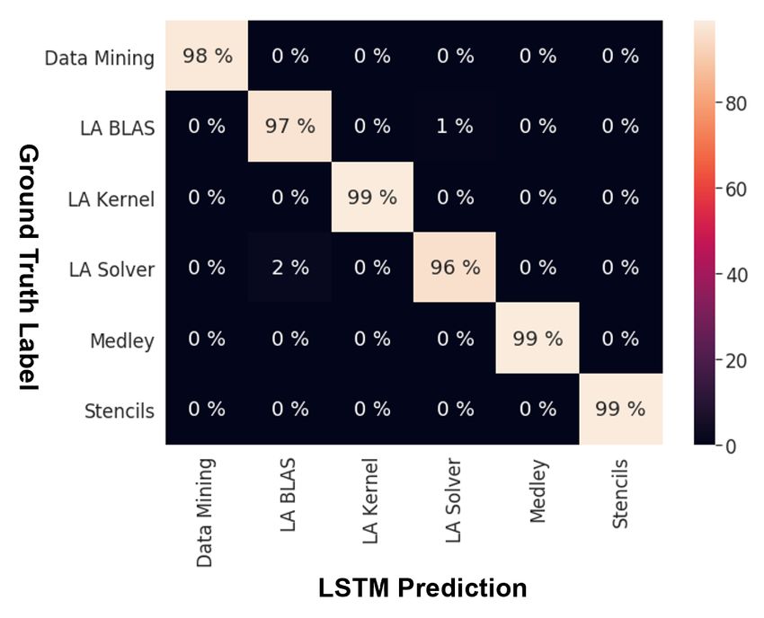
Contents
List of Figures                                                                                                              ii

List of Tables                                                                                                               iii

1 Executive Summary                                                                                                           1

2 Introduction                                                                                                                2

3 Methods, Assumptions and Procedures                                                                                         3
  3.1 Intrepydd Programming Model . . . . . . . .        .   .   .   .   .   .   .   .   .   .   .   .   .   .   .   .   .    3
      3.1.1 Summary of Intrepydd v0.2 features . .       .   .   .   .   .   .   .   .   .   .   .   .   .   .   .   .   .    4
      3.1.2 Summary of Intrepydd v0.3 extensions         .   .   .   .   .   .   .   .   .   .   .   .   .   .   .   .   .    4
  3.2 Knowledge Base . . . . . . . . . . . . . . . . .   .   .   .   .   .   .   .   .   .   .   .   .   .   .   .   .   .    5
  3.3 Static Data-aware Optimizer . . . . . . . . . .    .   .   .   .   .   .   .   .   .   .   .   .   .   .   .   .   .    7
  3.4 Dynamic Kernel Reoptimizer . . . . . . . . . .     .   .   .   .   .   .   .   .   .   .   .   .   .   .   .   .   .    8
  3.5 Auto-tuning and Reconfiguration system . . .       .   .   .   .   .   .   .   .   .   .   .   .   .   .   .   .   .   12

4 Results and Discussion                                                                                                     15
  4.1 Phase 1 performance evaluation approach and results . . . . . . . . . . . . .                                          15
      4.1.1 Efficient Architecture Performance Models based on CPU Hardware
             Performance Monitors . . . . . . . . . . . . . . . . . . . . . . . . . .                                        15
      4.1.2 Performance Evaluation for Phase 1 Workflows on Surrogate Model .                                                16
  4.2 Experimental Results on Standard CPUs . . . . . . . . . . . . . . . . . . . .                                          17
      4.2.1 Benchmarks . . . . . . . . . . . . . . . . . . . . . . . . . . . . . . . .                                       17
      4.2.2 Experimental Setup . . . . . . . . . . . . . . . . . . . . . . . . . . . .                                       18
      4.2.3 Comparison with Python, Numba, Cython for Single-core Execution .                                                19
      4.2.4 Impact of Parallelization . . . . . . . . . . . . . . . . . . . . . . . . .                                      21
      4.2.5 Comparison with Julia . . . . . . . . . . . . . . . . . . . . . . . . . .                                        22
  4.3 Phase 1 SLOC evaluation approach and results . . . . . . . . . . . . . . . .                                           22

5 Conclusions                                                                                                                24

6 References                                                                                                                 25

7 List of Symbols, Abbreviations, and Acronyms                                                                               27

                                              i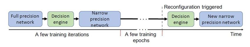
List of Figures
  1    Overview of ddaring programming system. . . . . . . . . . . . . . . . . . .            2
  2    Design of Intrepydd tool chain for -host=python mode . . . . . . . . . . . .           3
  3    Tripartite Representation of Knowledge Base . . . . . . . . . . . . . . . . . .        5
  4    Original data distribution for dataset1 . . . . . . . . . . . . . . . . . . . . .      8
  5    Results of KMeans . . . . . . . . . . . . . . . . . . . . . . . . . . . . . . . .      8
  6    Results of DBSCAN . . . . . . . . . . . . . . . . . . . . . . . . . . . . . . .        8
  7    Manual system overview . . . . . . . . . . . . . . . . . . . . . . . . . . . . .       9
  8    PyTorch extension . . . . . . . . . . . . . . . . . . . . . . . . . . . . . . . .      9
  9    Potential memory savings . . . . . . . . . . . . . . . . . . . . . . . . . . . .      10
  10   Potential compute savings . . . . . . . . . . . . . . . . . . . . . . . . . . . .     10
  11   Overview of auto precision tuning system . . . . . . . . . . . . . . . . . . . .      10
  12   Decision engine overview . . . . . . . . . . . . . . . . . . . . . . . . . . . . .    11
  13   Integer precision system overview . . . . . . . . . . . . . . . . . . . . . . . .     11
  14   Opportunity for Data Width Savings . . . . . . . . . . . . . . . . . . . . . .        12
  15   Error matrix of the test set constructed with seen applications . . . . . . . .       13
  16   Output from different stages of phase detection . . . . . . . . . . . . . . . .       14
  17   Relative modelling speed vs. accuracy of RTL, cycle accurate and surrogate
       modeling. . . . . . . . . . . . . . . . . . . . . . . . . . . . . . . . . . . . . .   16
  18   Comparison of Intrepydd and Python using the surrogate model . . . . . . .            17
  19   Single core performance improvements for primary kernels relative to Python
       baseline (derived from data in Tables 3 and 4) . . . . . . . . . . . . . . . . .      19
  20   Multi core scalability of intrepydd for a subset of the benchmarks in host=cpp
       mode. The Performance Improvement Factor is relative to the single-core
       execution time in host=python mode. . . . . . . . . . . . . . . . . . . . . . .       21

                                            ii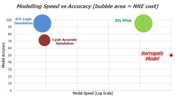
List of Tables
  1   Runtime prediction results for top three SDH kernels – Mean Absolute Error
      (Mean Absolute Percentage Error), Training Time. . . . . . . . . . . . . . . .       6
  2   Benchmark characteristics . . . . . . . . . . . . . . . . . . . . . . . . . . . .   17
  3   Average single core execution times (in seconds) and standard deviation of
      10 runs as a percentage of average execution times (in parenthesis) for the
      baseline Python (times for overall benchmark and primary kernel). . . . . . .       18
  4   Average single core execution times (in seconds) and standard deviation of
      10 runs as a percentage of average execution times (in parenthesis) for the
      primary kernel written in each of Cython, Numba, unoptimized intrepydd,
      and optimized intrepydd. . . . . . . . . . . . . . . . . . . . . . . . . . . .      18
  5   Average single core execution times (in seconds) for the primary Benchmark ker-
      nels written in intrepydd and compiled with increasing sets of optimizations:
      unoptimized, +LICM (Loop-Invariant Code Motion), +Sparse/Dense Array
      optimizations (Array Operator Fusion), +Memory Allocation Optimizations.            20
  6   Average single core execution times (in seconds) for Python, Julia and in-
      trepydd versions of four benchmarks. . . . . . . . . . . . . . . . . . . . . .      22
  7   SLOC of workflows . . . . . . . . . . . . . . . . . . . . . . . . . . . . . . . .   23

                                            iii
1 Executive Summary
DARPA’s program on “Software Defined Hardware” (SDH) put forth a grand challenge to
build runtime-reconfigurable hardware (TA1) and software (TA2) that enables near ASIC
performance without sacrificing programmability for data-intensive algorithms. As a TA2
performer, the ddaring team addressed this challenge in Phase 1 of the SDH program by
introducing multiple software innovations for future hardware with programmability that
is comparable to what data scientists expect today. The results of our research have been
published in 16 peer-reviewed publications [1–16]. As described in these publications, and in
this report, the main advances have been in the following areas:
1. As described in Section 3.1, we designed and implemented a new Python-based program-
ming model, called Intrepydd, that is suitable for ahead-of-time compilation. Depending
on the mode selected during compilation, code generated from Intrepydd programs can
be integrated within a Python application, or a C++ application. The first mode was
used by testers in the Phase 1 programmability evaluations who were given access to
the Intrepydd v0.2 toolchain via a docker container, and the second mode was used to
enable code generation for the simulator developed by our TA1 partner (which does
not support a Python runtime environment).
2. We also designed and implemented the first version of the ddaring knowledge base,
summarized in Section 3.2, with the goal of learning and storing extensive information
on (a) mapping of workflow “steps” to “kernels”, and (b) mapping of kernels to available
hardware configurations.
3. Section 3.3 summarizes our work in Phase 1 on static code optimizations. The approaches
that we have taken to multi-version code generation promises to advance state of the
art in data-aware code optimization, as demonstrated in our results for the Word2Vec
workflow and data clustering workflows.
4. Section 3.4 summarizes our early work on extending the foundations of dynamic code
optimization, with demonstrations of opportunities for automatic tuning of floating-
point precision in deep learning workflows as well as reduction of fixed-point precision
in important integer applications.
5. Finally, Section 3.5 summarizes the advances that we have made in using various
machine learning techniques for key tasks that need to be performed by an online auto-
tuner, including identifying the application domain of the currently executing kernel,
detection of a phase change in execution characteristics, and selection of optimized code
and hardware configurations.
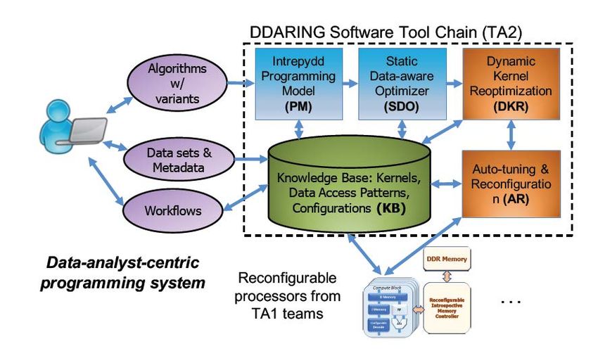
Our results show that the DDARING programming system has made significant progress
towards the SDH program goals in Phase 1. The programmability of the Intrepydd tool chain
is already close to that of Python. Further, our toolchain, in Phase 1, has already bridged a
large fraction of the typical orders-of-magnitude gap between Python and theoretical peak
performance. In Section 4.1, we used the “surrogate model” approach to approximately
estimate execution time, energy and GOPS/Watt metrics on SDH hardware for Intrepydd
Approved for Public Release; Distribution Unlimited.
1and Python implementations. The performance evaluations using the surrogate model
showed 130.2× geometric mean speedup and 314.1× geometric mean energy efficiency by the
Intrepydd implementations, compared with the Python implementations.
Further, the performance evaluations on dual Intel Xeon Silver 4114 CPUs with 10
physical cores per CPU socket were performed. We compare the single-core performance
of Python, Cython, Numba, unoptimized intrepydd, and optimized intrepydd for six
SDH workflows that span different data science domains summarized in Table 2. One of
these benchmarks was chosen because it is dominated by native library calls in its execution
time, and the other five are non-library-dominated benchmarks. As shown in Figure 19, the
optimized intrepydd version in host=python mode shows performance improvements in
the range of 11.1× to 8809.8× for the five non-library-dominated benchmarks, and of 1.5×
for the library-dominated benchmark, compared to baseline Python. Similarly, the optimized
intrepydd in host=python mode shows 1.5× - 50.5× of performance improvements over
existing state-of-the-art techniques, Cython and Numba. We also evaluated the parallel
performance for four of the six benchmarks that were candidates for using intrepydd’s
pfor construct, on a dual socket Intel Xeon E-2680 V4 (14 cores per socket). As shown in
Figure 20, the optimized intrepydd in host=cpp mode shows 2.0× - 8.0× speedups using
16 cores, with respect to the sequential optimized intrepydd.
2 Introduction
Figure 1: Overview of ddaring programming system.
As a TA2 effort, the ddaring project aims to advance the SDH program goals by
developing a novel programming system for generating optimized code variants and optimized
hardware configurations for TA1 hardware platforms. Figure 1 shows an overview of our
technical approach with the overall goal of accelerating workflows for data-intensive analyses
Approved for Public Release; Distribution Unlimited.
2to achieve near-ASIC performance, but with the productivity that analysts have come to
expect from modern problem-solving environments such as Julia and Python. As illustrated
in Figure 1 and described below, we have developed in Phase 1 a new high-level programming
model (Section 3.1), a knowledge base (Section 3.2), a static data-aware optimizer (Section 3.3),
a dynamic kernel reoptimizer (Section 3.4), and an auto-tuning and reconfiguration system
(Section 3.5).
3 Methods, Assumptions and Procedures
3.1 Intrepydd Programming Model
Figure 2: Design of Intrepydd tool chain for -host=python mode
Intrepydd is a new analyst-friendly Python-based programming model suitable for ahead-
of-time (AOT) compilation on current and future hardware platforms and accelerators,
thereby enabling “performance programming” in a lightweight Python syntax. It builds on
an AOT-compilable subset of Python with extensions for matrix, tensor, graph, and deep
learning computations that expose opportunities for dynamic data-aware code optimizations
and hardware reconfiguration.
Intrepydd is not intended for writing complete/main programs. Instead, code gener-
ated from Intrepydd programs can be integrated within a Python application (with the
-host=python mode) or within a C++ application (with the -host=cpp mode). Intrepydd
was designed from scratch for the SDH program. Figure 2 summarizes the design of the
Intrepydd tool chain for -host=python mode.
We released v0.2 of Intrepydd in end-May for use in the Phase 1 programmability evaluation
and developed v0.3 after that as the latest version used to obtain the Phase 1 evaluation
results presented later in this report. A list of v0.2 features is summarized below, followed by
a summary of the extensions in v0.3.
Approved for Public Release; Distribution Unlimited.
33.1.1 Summary of Intrepydd v0.2 features
Intrepydd v0.2 only supports the -host=python mode, and encourages incremental use of
Intrepydd within a familiar Python ecosystem, including Jupyter notebooks and standard
Python profiling tools. A programmer creates an Intrepydd module in a file with a .pydd
extensions, and invokes the Intrepydd compiler, pyddc, to enable AOT compilation. A key
requirement in Intrepydd v0.2 is that all function parameters and return values must be
declared with explicit types. Intrepydd code can be invoked from Python by importing the
Intrepydd module, similar to importing a Python module. Examples of Intrepydd code are
provided in Section 4.3.
Intrepydd v0.2 supports bool, int32, int64, float32, and float64 as primitive types,
as well as dense arrays, sparse arrays, and lists of primitive types. These data types are
inferred automatically for local variables and expressions, based on the type declarations
provided for parameters and return values. In some cases, explicit type declarations may
be needed for assignment statements by using Python’s PEP 484 type annotation with the
“var: Type” syntax. Support for other type annotations, e.g., PEP 526, is deferred to future
versions of Intrepydd.
Intrepydd v0.2 also supports the following standard statement types from Python: assign-
ment statements, function calls, return statements, sequential for and while loops with break
/ continue statements, and conditional if/elif/else statements. In addition, Intrepydd v0.2
supports a parallel for (pfor) loop statement, which is not available in Python. Intrepydd
expressions can be constructed using a large set of unary and binary operators on scalars and
arrays, as well as list constructors and array element operators.
There are some documented syntactic limitations in v0.2 of Intrepydd, which will be
addressed in future releases. Certain Python array operators need to be replaced by alternate
Intrepydd function calls in v0.2, e.g., + → add(), / → div(), * → mul(), @ → matmult() or
spmm(), len(x) → x.shape(0), a:b → range(a,b). In addition, NumPy calls need to be replaced
by generic calls so that it is possible to compile Intrepydd code with no NumPy dependencies
in the -host=cpp mode, e.g., np.zeros() → zeros(), np.sqrt() → sqrt(). Finally, some
currently unsupported Python calls have to be replaced by explicit code, e.g., sum(axis=. . . )
→ reduction loop, append() → append loop, maximum() → code to compute max, and
replacement of an unsupported allocation function by a call to a supported allocation function
followed by updates to the allocated array.
3.1.2 Summary of Intrepydd v0.3 extensions
The Intrepydd v0.3 implementation extends Intrepydd v0.2 with the following features:
addition of SparseMat as a builtin type for sparse matrices, enhanced type inference so
that function return types can be automatically inferred, removal of some of the syntactic
limitations in v0.2, improved error messages from the pyddc compiler, and command-line
options such as specifying compiler/linker flags. Further, a new loop invariant code motion
(LICM) optimization was added that can also be applied to array operators, instead of
just scalar operators as in traditional compiler implementations of LICM. Finally, a num-
ber of additional built-in wrappers were added for popular libraries for arrays including:
where(), element-wise logical and max operations, sparse array creation from dense vectors,
Approved for Public Release; Distribution Unlimited.
4sum(axis=. . . ) reduction on an axis, and builtin support for the heap data structure.
3.2 Knowledge Base
The goal of the knowledge base is to enable the acceleration of workflows by storing and
learning extensive information on (a) mapping of workflow “steps” to “kernels”, and (b)
mapping of kernels to available hardware configurations.
Representation
Figure 3: Tripartite Representation of Knowledge Base
The knowledge base comprises of a rich tripartite graph representation G(V1 , V2 , V3 , E)
(TGR) as shown in figure 3. The first layer V1 consists of Domain-Specific Language level
(DSL) steps. A step is a pattern of computation that can be mapped to one or a combination
of kernels. The set V1 is the steps discovered in a codebase which includes a wide range
of data-intensive workflows. Each u ∈ V1 is attributed with a feature D to quantitatively
represent computational and data access patterns of the step (or part of the workflow) such
as access pattern irregularity, data precision, computation to communication ratio, etc. A
workflow is a finite-state-machine of the steps in V1 . Nodes in set V2 represent bare bone
tasks or kernels that form the core of the knowledge base. A step may have multiple variants
in terms of kernels. For instance, a convolution operation can be represented as 1) a sequence
of frequency domain transformation, multiplication and inverse transformation steps, or 2) a
series of sliding window dot products. Frequently co-occurring kernels may be merged to form
one kernel for optimized implementations. The kernels K ∈ V2 are mapped to the underlying
building blocks of the hardware platform. The hardware configurations and building blocks
are represented as vertices v ∈ V3 . Note that a kernel can be mapped to one hardware
configuration (T , C) in multiple ways (T ) with different performance costs (C). This is
Approved for Public Release; Distribution Unlimited.
5desirable as it would provide ways to schedule a task even if the optimal hardware block for
execution is busy. Vertices in V3 also store their cost of reconfiguration, which is taken into
account while computing the optimal mapping and overall cost of kernel execution. We have
partially populated the knowledge base using execution profiles from SDH workflows.
Learning Kernel-to-Hardware Performance Models
The performance models are designed to be trained on the target hardware. We want these
models to be small so that when the knowledge base is bootstrapped on a new machine, it
can run some benchmarks to train performance models for a set of kernels quickly. Currently,
we have built prediction models for three operations: Matrix-Matrix Multiplication, Matrix-
Vector Multiplication, and Convolution. We perform the modeling for each of these kernels,
and then train it on the desired hardware. For a given kernel, the model remains fixed, while
the parameters, i.e., the weights differ over different hardware. Our model is a compact
neural network, augmented with mathematical formulae for complexity for the kernel, for e.g.,
Cn1 n2 n3 for multiplying matrices of size n1 × n2 and n2 × n3 ; C is a constant learned through
training. Overall the number of parameters are kept under 75 and training is performed
with 250 samples only for each kernel-hardware pair to ensure small memory footprint and
fast training. The models only take input dimensions and matrix densities as input and
output the predicted runtime. Table 1 shows the prediction results from our approach1 . Our
approach significantly outperforms baselines, including neural networks (without complexity
augmentation) and linear regression. We also obtained up to 1.3× higher accuracy with
larger models (∼ 1000 parameters) and larger data (∼10000 samples) but have omitted the
results as they are not practical due to slow training and large memory requirement.
Table 1: Runtime prediction results for top three SDH kernels – Mean Absolute Error (Mean
Absolute Percentage Error), Training Time.
Operation Intel(R) Intel(R) Core Intel(R) Tesla K40c Quadro K420
Core i7- i5 CPU @ Xeon(R)
8750H CPU 2.30GHz CPU E5-
@ 2.20GHz 2650 v2 @
2.60GHz
Matrix- 0.06s 0.06s 0.04s 2.36 ∗ 10−4 s 2.36 ∗ 10−4 s
Matrix (30.35%) (21.75%) (25.85%) (14.95%) (9.72%)
3min 3min30s 2min30s 10.76s 10.56s
Matrix- 2.76 ∗ 10−4 s 7.52 ∗ 10−4 s 4.25 ∗ 10 s 1.15 ∗ 10−5 s
−4
1.22 ∗ 10−5 s
Vector (12.32%) (19.81%) (8.03%) 2min (7.00%) 7.31s (7.96%) 7.79s
2min 2min
Convolution 0.05s 0.02s 0.04s 7.79*10-5s 1.22 ∗ 10−4 s
(24.88%) (10.51%) (12.26%) (9.63%) 15s (15.07%)
2min30s 2min30s 4min 13.7s
1
While Section 4 presents and discusses detailed end-to-end results for our approach, we also include some
per-component results in Section 3 to aid in the presentation of methods, assumptions and procedures.
Approved for Public Release; Distribution Unlimited.
63.3 Static Data-aware Optimizer
Our approach to static data-aware optimization is founded on multi-version code generation,
which can have benefits in at least two ways: 1) generating specialized code for different
classes of data inputs, and 2) selecting the best algorithmic strategy for a given data input.
Below, we summarize our work on optimizing the Word2Vec workflow as an illustration
of 1), and our work on optimizing data clustering workflows as an illustration of 2). Both
optimization approaches are enabled by high-level semantic information in the Intrepydd
programming model.
Code specialization for the Word2Vec workflow
Word2Vec is an SDH workflow, and an important kernel in Natural Language Processing
(NLP). It is widely used to embed words from textual data in a vector space. Previous work
improved the performance of the original Word2Vec implementation by converting vector-
vector operations to matrix-matrix operations and using state-of-the-art BLAS routines for
the resulting level-3 BLAS operations. This conversion effectively batches inputs and shares
the same negative samples across a batch of inputs. However, many performance overheads
remain in his approach because a) many of the matrix sizes have highly nonuniform aspect
ratios that are not well suited to BLAS, e.g., tall and skinny matrices, and b) we make several
library calls for consecutive operations, which reduces register reuse. These overheads motivate
the generation of multi-version code for different matrix sizes. Our preliminary results show
significant performance improvement over the state-of-the-art Word2Vec implementation on
x86.
In our evaluation, we used the Skip-Gram with Negative Sampling (SGNS) for Word2Vec.
We statically generated multi-version code specialized on two parameters - number of inputs
and number of outputs - so that the appropriate specialized code can be chosen at runtime
based on the parameter values for each call. Our evaluation was performed on the widely
used Billion Word Language Model Benchmark, with a word vector length of 300, a window
size of 5 (which implies that the number of inputs can vary from 1 to 10), and 5 negative
samples (which implies that the number of outputs can vary from 1 to 6). This results in
60 possible combinations for the number of inputs, M , and the number of outputs, N . The
specialized code generated by our system was observed to be 1.78× to 5.71× faster than the
state of the art across all 60 combinations. The largest performance improvement of 5.71×
was observed for (M, N ) = (2, 4) and the smallest improvement of 1.78× was observed for
(M, N ) = (8, 6).
Algorithm selection in Data Clustering workflows
Going beyond code specialization, a higher-level optimization opportunity can be found in
algorithm selection. For example, KMeans, DBSCAN, KNN, PCA are a few choices for
data clustering algorithms. The ideal choice of algorithm can depend on the data input
and the target hardware, and a poor choice can impact the accuracy or performance of
the workflow. In this preliminary work, we sought to automate the selection of Kmeans vs.
DBSCAN algorithms to solve data clustering problems with different inputs. The goal of
our approach is to build an efficient library that automatically selects among KMeans and
Approved for Public Release; Distribution Unlimited.
7Figure 4: Original data Figure 5: Results of
Figure 6: Results of DBSCAN
distribution for dataset1 KMeans
DBSCAN algorithms. To improve the effectiveness of the library, we adopt a sub-sampling
method to choose between the two clustering algorithms; sub-sampling method reduces the
cost of executing the two candidate clustering algorithms on a given data set. Currently, our
library works with data sets containing two-dimensional data points.
Two data sets were used for testing the algorithm selection library and analyzing scenarios
when one of the clustering algorithms would be better than the other one. Figure 4 shows
the original data distribution of the given dataset, which dataset was generated using the
scikit module. Our subsampling approach suggested that the Kmeans algorithm (Figure 5)
would yield a better result than DBSCAN (Figure 6), thereby selecting the better algorithm
with low overhead since subsampling was performed on a dataset that was 0.1% of the size of
the actual input data set in Figure 4.
3.4 Dynamic Kernel Reoptimizer
Deep Neural Networks Training Precision Tuning
Researchers have shown that DNNs are able to preserve accuracy while operating with
reduced precision data formats. Using narrow precision operations has two main benefits: (1)
Reducing the number of memory accesses. (2) Increasing the throughput with SIMD-like
operations. As a result, it is possible to gain energy savings and speedups by performing DNN
computations in a narrow precision format. As the required bit-width varies among different
networks and layers, a dynamic precision tuning system is needed in order to maximize
savings while preserving the network’s accuracy. Although both reduced precision training
and inference are active fields of research, our main focus is on the training phase because it
runs longer and is more compute and memory intensive than inference. In this report, first,
we examine the potential benefits of narrow precision computation during the training. After
that, we propose a design to tune a network’s precision automatically during training while
maintaining its accuracy.
Manual Precision Exploration:
In this section, we discuss our tool, which allows us to run the input network with a user-
defined precision configuration (Figure 7). The user must declare the layer-wise network
configuration before training. Once training is complete, the user can evaluate the trained
network and reconfigure the precision if desired. By repeating this procedure, the user can
Approved for Public Release; Distribution Unlimited.
8find the narrowest precision that preserves the accuracy of the network. It is possible to set
an arbitrary precision for each layer, and this precision can vary among different epochs.
Train the network
Set the network Evaluate the
using user-defined
configuration trained network
configuration
Figure 7: Manual system overview
The PyTorch framework does not support arbitrary precision operations. Thus, we had
to add arbitrary precision computation capability to the framework. Each of PyTorch’s
three implementation layers had to be re-implemented. Figure 8 shows a high-level block
diagram of the PyTorch extension. The first level is CUDA, which has all the computationally
intensive kernels. The second one is the CPP Wrapper, which prepares the input data of
the computation kernels. The last one is the PyTorch Frontend, which is a wrapper for the
CPP code and provides the interface to the user. The CUDA kernels are able to perform
computations in arbitrary precision.
Arbitrary Precision
PyTorch Code
Python
Frontend
PyTorch Libraries Extension
CPP
Wrapper
Pre-compiled
Extension
BLAS Libraries
CUDA
Backend
Figure 8: PyTorch extension
Using this tool, we were able to calculate potential savings in multiple benchmarks. Figure
9 compares the potential memory savings in three different scenarios. First, saving all the
parameters in half float format, which does not guarantee the network’s accuracy. Second,
performing all the training using one precision for each layer of the network, named “Dynamic
One Width”. Third, finding the narrowest precision for each layer per epoch and dynamically
changing the precision, named “Dynamic Multi Width”. Dynamic One Width is not achievable
as it needs to know the precision requirement of each layer during the training beforehand of
starting the process. Our proposed idea is Dynamic Multi Width, which outperforms all the
other methods.
Figure 10 compares the amount of computation required for the full precision and reduced
precision formats, assuming that computational units are fully dynamic and are able to
perform arbitrary precision.
These results are promising and motivate us to work on a tool that tunes the precision
automatically.
Approved for Public Release; Distribution Unlimited.
96
5
Model Size (MB)
4
3
2
1
0
MNIST - LeNet 5 MNIST - WideNet CIFAR-10 - LeNet 5 CIFAR-10 - ConvNet
Full Precision Half Float Dynamic One Width Dynamic Multi Width
Figure 9: Potential memory savings
60
Computation Required (MFLOPS)
50
40
30
20
10
0
MNIST - LeNet 5 MNIST - WideNet CIFAR-10 - LeNet 5 CIFAR-10 - ConvNet
Full Precision Half Float Dynamic One Width Dynamic Multi Width
Figure 10: Potential compute savings
Dynamic Precision Reconfiguration:
As mentioned in the previous section, having an automatic tool that finds the best precision
configuration while the training is going on is required in order to train arbitrary networks
efficiently. Figure 11 shows an overview of the proposed system, which periodically reevaluates
the best precision configuration for the network every few epochs of training. In this automatic
system, the user has no role to play and retraining the network is not required.
Figure 11: Overview of auto precision tuning system
Whenever precision reconfiguration is required, the decision engine (Figure 12) routine is
called. The decision engine clones the original network to multiple candidate networks that
have the potential to have the best precision configuration. After training all the networks
Approved for Public Release; Distribution Unlimited.
10for a few iterations, the decision engine evaluates candidates based on different metrics
(direction of weights update, the loss value, etc.) and finds the configuration which has the
best precision. After that, the network will be trained with the chosen candidate configuration
until the next time the decision engine is called. As wrong decisions from the decision engine
might cause divergence during the training process, the system has a check-pointing based
recovery strategy. This system is currently in progress.
Full precision
After a few
Candidate training iterations
precision #1 Evaluate narrow Candidate
Candidate precision candidates precision #i
precision #2 Returns the candidate network
.. which meets requirements
.
Candidate
precision #N
Figure 12: Decision engine overview
Integer Precision Reduction
Figure 13: Integer precision system overview
As shown in Fig. 13, the dynamic integer precision reduction system has two components:
the dynamic compiler and the hardware. The compiler will use profiling and application
information from the knowledge base to decide on appropriate data widths for storage and
operations. To reduce the overhead of the profiling step, the functionality could be added to
identify code regions amenable to precision reduction, so values from the entire program do
not have to be sampled.
The hardware will pack and unpack data from memory on loads and stores according to
the compiler-chosen data width. This allows for potential savings in the memory system as
fewer memory and cache accesses will be needed for the same amount of data. Once the data
is in the register file, we can perform operations in the reduced width and recover if we are
too aggressive. The key insight is that we can use the already existing overflow bit in modern
processors to detect a data width violation in integer computation.
Approved for Public Release; Distribution Unlimited.
11Figure 14: Opportunity for Data Width Savings
To motivate the dynamic integer precision reduction system, we see in Fig. 14 that
four prominent integer applications: constraints solving (SAT), genomic sequencing, video
encoding, and video decoding on average leave about 60% of their data widths unutilized.
The Dynamic One-Width shows the potential data width savings if each instruction only uses
its maximum required width over the course of execution, and the Dynamic Multi-Width
shows potential savings if the instruction width could perfectly adapt to the needs of the data.
Note that these two metrics are oracles and can only be found after processing is complete
as precision is dependent on the input data. Based on these preliminary results, in Phase
2, our goal will be to evaluate the system and provide performance and energy results in
simulation for existing hardware with minor modifications. The results will then be extended
to hardware with fast reconfiguration times to showcase the additional gains that an SDH
machine could provide.
3.5 Auto-tuning and Reconfiguration system
This section summarizes the advances that we have made in using various machine learning
techniques for key tasks that need to be performed by an online auto-tuner, including
identifying the application domain of the currently executing kernel and detection of a phase
change in execution characteristics. Due to space limitations, we omitted text on our approach
to the selection of optimized code and hardware configurations, which was also presented at
the recent SDH PI meetings.
Application Domain Detection
In ddaring, we define the application domain as a group of programs that shares similar
characteristics and serves a similar purpose. For example, matrix decomposition, such as LU ,
Cholesky, P DP −1 , are likely to be in the same application domain, since they consist of
similar matrix manipulation operations and are all usually used for solving linear systems.
To identify the application domain of a given program, we first capture the behavior of
the application by profiling and collecting data from performance counters in the processor’s
performance monitoring unit (PMU). We then use a Long Short-Term Memory (LSTM)
classifier that operates on sequences of PMU data collected from a real machine. In the
Approved for Public Release; Distribution Unlimited.
12Figure 15: Error matrix of the test set constructed with seen applications
following subsections, we will describe the data we collected, how we process the raw data to
create a dataset, and how we train and evaluate the LSTM model.
Data Acquisition and Pre-processing:
To collect all the raw data from the performance counters, we utilized the perf tool on
Linux distributions. The processor in the test system that we used is an Intel CPU with 53
performance counters available. Due to the limitation of the processor and the profiling tool,
we were not able to collect all the values at once, so we have to collect only 5-7 counters at a
time, and use time multiplexing to collect all counter values. We used a sampling interval of
100ms due to system limitations, but we assume that the target SDH hardware will be able
to support much higher sampling rates.
Model Construction and Training:
LSTM is a type of recurrent neural network (RNN) that specializes in detecting long-term
relationships of sequential data. It has shown impressive performance on a variety of tasks such
as speech-recognition and neural machine translation. Since the classification of sequences of
performance data is conceptually similar to these tasks, we believe that LSTMs will work
well for our purpose.
We implemented the LSTM with the popular PyTorch framework with the help of
scikit-learn and Numpy on preprocessing and dataset construction. Since one of the main
requirements of the application domain detection, in the context of ddaring, is to detect the
domain without large run-time overhead, we limited the size of the neural network for faster
inference and lower resource consumption. Our final model consists of a single layer LSTM
with 128 hidden units, and a single classification layer for generating the final classification.
For this evaluation, the number of output classes is 6, and correspond to the application
classes identified in [17]. In the future, we plan to expand the application classes for increased
coverage of SDH workflows. For simplicity, we use regular stochastic gradient descent for
training and set the learning rate to 0.01 for faster convergence. In our experiments, we
didn’t observe significant over- or under-fitting. We did the training and evaluation with
an Nvidia GTX1080 GPU, and the model is trained for 35 epochs, which takes around 5
Approved for Public Release; Distribution Unlimited.
13(a)
(b)
(c)
Figure 16: Output from different stages of phase detection
minutes. Note that the time might vary depending on the system configuration and the code
implementation.
Evaluation and Results:
The results show that on the test set, the LSTM can correctly classify 98% of the sequences.
The error matrix presented in Figure 15 shows that it can correctly classify 99% of the
sequences from most of the domains. The only non-zero entries occur for linear algebra
classes that exhibit similar characteristics (LA BLAS and LA Solver).
Program Phase Detection
Dynamic reconfiguration is one of the most important features of ddaring. In reality, the
applications can have multiple program phases, in which the performance and behavior of
the system are relatively steady. During these periods, the system can be reconfigured to
adapt to the characteristics of the phase to achieve better efficiency. Therefore, we need to
identify the changes in the phases to identify the best opportunity for reconfiguration.
For this purpose, we developed a technique to detect the change of the program phase
by using the data collected from the performance counters. The core of this technique is to
leverage an unsupervised learning algorithm, namely k-means clustering, to automatically
identify the steady periods of program execution.
Approved for Public Release; Distribution Unlimited.
14The first step of phase detection is data collection. Similar to the application domain
detection, we collect the data from the performance monitoring units (PMU). However, there
are 53 different counter values in the raw data, and this high dimensionality makes it difficult
to further process the data. Therefore, we then apply principal component analysis (PCA)
to reduce the dimension of the input and extract the most important information. PCA
is a popular feature extraction algorithm that can transform the high dimension input to
a low dimension representation with the magnitude of the principal components (PC). It
is especially helpful for clustering algorithms since the clustering algorithms suffer from
the ’curse of dimensionality’ that makes them less effective. We noticed that most of the
important information is captured by the magnitude of the first principal component. Figure
16a illustrates the magnitude of the first component of the for all samples in the data collected
for the ’3mm’ (3 consecutive matrix multiplications of different sizes) benchmark in Polybench
benchmark suite. The x-axis of the diagram is the index of the sample in time order, and the
y-axis is the magnitude of the PC; the red dotted line represents the actual division between
phases. As we can see, there are three human-identifiable phases, which correspond to the
three matrix multiplications.
However, simply applying PCA is not enough to detect the phases. Notice that the
output of PCA has a large number of noise peaks, and these peaks might be identified as
separate phases by the unsupervised learning algorithm. Therefore, we apply median filtering
to remove the peaks. It replaces the value of a sample with the median within the sliding
window, so the large peaks with extreme values will be removed. After applying the filter, as
shown in figure 16 (b), the phases can be observed much easier.
Finally, since the phase detection process needs to output logical labels for the phases, we
applied the k-Means clustering algorithm to group the data points into clusters where each
cluster represents a unique phase. To determine the optimal number of clusters automatically,
we applied grid search and use Silhouette score as the criteria, and after this step, clear
phases can be detected and are tagged with logical phase label. In figure 16 (c), the y-axis is
the logical phase label (the magnitude of it does not have any indication), and we can see
that there are three phases which align with the phases that human can identify from figure
16.
4 Results and Discussion
4.1 Phase 1 performance evaluation approach and results
4.1.1 Efficient Architecture Performance Models based on CPU Hardware Per-
formance Monitors
In general, there are two approaches to the problem of performance modeling for future
architectures. One is to actually construct the RTL of the design. This is of course highly
accurate, including precise estimates of energy and power. Speed of evaluation is variable:
one can synthesize into an FPGA (very fast) or perform a software logic-level simulation
(very slow) But this approach has very high NRE cost.
The other approach is so-called “cycle accurate” simulation models. These are constructed
often from the architect’s understanding of the system. Often these are implemented using
Approved for Public Release; Distribution Unlimited.
15event-driven approaches. While they have much lower development time, they are very slow
to evaluate.
In Phase 1, we have developed a third approach called a surrogate model. Here an
application is run on an existing architecture. The performance counters of events relevant
to the target architecture are collected during the run. (For example, native DRAM CAS
read and write events may be mapped to transactions on the memory bus in the target
architecture.) A model is constructed to translate these events into performance and energy
estimates of the target architecture. This approach allows a programmer to get virtually
instant feedback. Such feedback is vital in enabling applications to be developed in parallel
with the target architectures. The relative modeling speed vs. accuracy of these approaches
are shown in Figure 17.
Figure 17: Relative modelling speed vs. accuracy of RTL, cycle accurate and surrogate
modeling.
4.1.2 Performance Evaluation for Phase 1 Workflows on Surrogate Model
We developed a tool that uses the hardware performance counters on a native version 4 Xeon
Intel processor to record certain events (such as instruction count and lowest level cache miss
rate) in order to provide estimates of the run time, cache miss rate and energy on the target
TA1 architecture. In our testing, this proved to be within +/- 44%, on average, to the actual
numbers from the cycle accurate architecture simulator developed by our TA1 partner.
Using the surrogate model, we were able to demonstrate that Intrepydd (PYDD) signifi-
cantly improves the estimated energy and execution time relative to Python, as shown in
Figure 18. As the geometric mean improvements of the evaluated six workflows, the Intrepydd
implementations showed the speedup factor of 130.2 and the energy efficiency factor of 314.1
over the baseline Python implementations.
Approved for Public Release; Distribution Unlimited.
16Figure 18: Comparison of Intrepydd and Python using the surrogate model
Table 2: Benchmark characteristics
Workload Domain Description
bigCLAM Graph Overlapping community detection in massive graphs using the
BIGCLAM algorithm.
changepoint Graph Finds change points of a graph based on node properties
ipnsw Graph Non-metric Similarity Graphs for Maximum Inner Product Search
ISTA ML Local graph clustering (LGC) through Iterative shrinkage-
thresholding
PR-Nibble ML Uses the Page Rank algorithm to find local clusters without
traversing the entire graph
sinkhorn-wmd NLP Computes Word Movers Distance (WMD) using Sinkhorn distances
4.2 Experimental Results on Standard CPUs
In this section, we present an empirical evaluation of our implementation of the intrepydd
tool chain, which follows the methodology advocated in the SIGPLAN Empirical Evaluation
Checklist [18] to the best of our ability. Based on the results and their explanations included
below, our claim is that the intrepydd approach can deliver notable performance benefits
relative to current approaches available to Python programmers for improved performance,
namely Cython and Numba; further, these benefits are especially significant for Python
applications with execution times that are not dominated by calls to native libraries. We also
claim that there is no loss in productivity relative to current approaches, since intrepydd’s
requirement for declaring types of function parameters and return values is also shared by
Cython (which imposes additional limitations as well) and by Numba’s eager compilation
mode. Finally, we claim that intrepydd offers more portability than current approaches,
since different code versions can be generated from the same intrepydd source code using
the host=python and host=cpp modes.
4.2.1 Benchmarks
Given the focus of intrepydd on the data analytics area, we picked up two additional work-
flows, bigCLAM and changepoint from the SDH Workflows. Since the primary contribution
Approved for Public Release; Distribution Unlimited.
17Table 3: Average single core execution times (in seconds) and standard deviation of 10 runs
as a percentage of average execution times (in parenthesis) for the baseline Python (times for
overall benchmark and primary kernel).
Benchmark Python Benchmark times Primary Kernel execution times
bigCLAM 12.69 (2.25%) 12.36 (1.21%)
changepoint 20.89 (0.71%) 16.37 (0.65%)
ipnsw 21.07 (0.90%) 17.44 (1.61%)
ISTA 30.29 (0.28%) 27.37 (0.06%)
PR-Nibble 53.42 (1.23%) 52.84 (1.18%)
sinkhorn-wmd 48.17 (0.26%) 46.44 (0.08%)
Table 4: Average single core execution times (in seconds) and standard deviation of 10 runs
as a percentage of average execution times (in parenthesis) for the primary kernel written in
each of Cython, Numba, unoptimized intrepydd, and optimized intrepydd.
Benchmark Cython Numba intrepydd (Unopt.) intrepydd (Opt.)
bigCLAM 11.54 (1.31%) 4.157 (0.47%) 2.56 (3.60%) 1.09 (0.89%)
changepoint 119.64 (1.13%) 16.46 (0.48%) 1.47 (0.22%) 1.47 (1.23%)
ipnsw 17.03 (2.43%) 3.21 (0.59%) 1.68 (0.32%) 0.79 (0.18%)
ISTA 26.93 (0.09%) 30.62 (0.10%) 79.36 (0.06%) 18.51 (0.33%)
PR-Nibble 5.04 (0.45%) 3.27 (0.36%) 0.83 (0.84%) 0.006 (0.42%)
sinkhorn-wmd 46.82 (0.20%) 47.03 (0.05%) 47.61 (0.09%) 1.22 (0.40%)
of the current intrepydd implementation is to generate improved code, rather than to
improve libraries, we expect significant performance improvements primarily for applications
with execution times that are not dominated by calls to native libraries. We selected five
of these applications for use as benchmarks (bigCLAM, changepoint, ipnsw, PR-Nibble,
sinkhorn-wmd). For completeness, a sixth benchmark (ISTA) was also selected which spends
significant time in NumPy libraries, even though we do not expect significant performance
improvements for such programs.
The benchmarks are summarized in Table 2 and span three different domains in the data
analytics area – graph analytics, machine learning, and natural language processing. We are
unaware of any single DSL that covers all three domains, where as intrepydd can be used
for all of them given its broader coverage of the data analytics area.
4.2.2 Experimental Setup
All single-core experiments were performed on a machine with dual Intel Xeon Silver 4114
CPUs with 10 physical cores per CPU socket, running at a constant 2.2 GHz with 192
GB of main memory. Intel Turbo Boost was disabled. Our baseline for benchmark
comparison is Python version 3.7.6. All C/C++ code generated by intrepydd and
Cython (version 0.29.15) was compiled with GCC 7.5.0 using optimization level O3. The
Numba (version 0.48) and Cython benchmark source codes were written with a programma-
Approved for Public Release; Distribution Unlimited.
188809.74
50
Performance Imrprovement Factor over Python
40 38.05
Baseline (Single-Core)
30
22.18
20 16.15
11.38 11.13
10.48
10
5.43
2.98
1.02
1.07 0.14 0.99 1.02 0.89 1.48 0.99 0.99
0
bigCLAM changepoint ipnsw ISTA PR-Nibble Sinkhorn-wmd
Benchmark
Cython Numba PePPy (optimized, host=python)
Figure 19: Single core performance improvements for primary kernels relative to Python
baseline (derived from data in Tables 3 and 4)
bility similar to that of intrepydd, without any additional hand optimizations. For
Cython benchmarks, all kernel functions were annotated with @cython.boundscheck(False)
and @cython.wraparound(False), while for Numba, all functions were annotated with
@jit(nogil=True, nopython=True). Each benchmark was compiled once, and executed 11
times (with each run being launched as a new process, which included dynamic optimization
only in the case of Numba). The execution times reported for each data point is the average
latency of the later 10 runs from the set of 11 (the first run was omitted in the average). The
primary kernel execution times were measured at the Python invocation sites, and include
any overheads of native function calls. For single core experiments, each process was pinned
to a single-core in order to maintain a steady cache state and reduce variations between runs.
The normalized standard deviation for the averaged runs varied between 0.06% and 3.60%.
4.2.3 Comparison with Python, Numba, Cython for Single-core Execution
Tables 3 and 4 summarizes the results of our performance measurements of different single-
core executions of five versions of each benchmark: baseline Python, Cython, Numba,
unoptimized intrepydd, and optimized intrepydd. The first Python column includes
execution times for the entire application so as to provide a perspective on the fraction of the
application time spent in its primary kernel, which is reported in all successive columns. All
intrepydd executions were performed using the host=python mode, i.e., they all started
with a Python main program which calls the automatically generated code from intrepydd
as an external library. The optimized intrepydd version was obtained by applying the
following optimizations, which have been newly developed after the SDH Phase 1.
Approved for Public Release; Distribution Unlimited.
19Table 5: Average single core execution times (in seconds) for the primary Benchmark kernels written in
intrepydd and compiled with increasing sets of optimizations: unoptimized, +LICM (Loop-Invariant
Code Motion), +Sparse/Dense Array optimizations (Array Operator Fusion), +Memory Allocation
Optimizations.
intrepydd Primary Kernel execution times (seconds)
Benchmark UNOPT +LICM OPT +Array OPT +Memory OPT
bigCLAM 2.558 2.557 1.541 1.086
changepoint 1.472 1.469 1.466 1.471
ipnsw 1.679 0.786 0.786 0.786
ISTA 79.362 18.732 18.473 18.509
PR-Nibble 0.831 0.114 0.106 0.006
sinkhorn-wmd 47.612 47.395 1.225 1.220
• Loop-Invariant Code Motion (LICM) for standard operators and function calls.
• Dense/Sparse Array Operator Fusion with sparsity optimizations.
• Memory Allocation Optimizations:
– Reuse an allocated array across multiple array variables; and
– Access array slices via raw pointers instead of allocating new objects.
As mentioned earlier, the execution times for the five versions are for the primary kernel in
each benchmark. The full benchmark time for the baseline Python version is also provided
as a reference.
Figure 19 shows the performance improvement ratios for the primary kernels relative to the
baseline Python version, using the data in Tables 3 and 4. When compared to baseline Python,
the optimized intrepydd version shows improved performance ratios between 11.1× and
8809.8× for the five non-library-dominated benchmarks and 1.5× for the library-dominated,
ISTA benchmark. These are more significant improvements than those delivered by Cython
and Numba, thereby supporting our claim that intrepydd delivers notable performance
benefits relative to current approaches available to Python programmers. Further, optimized
intrepydd did not show a performance degradation in any case, though Cython and Numba
showed degradations in multiple cases (changepoint and ISTA). We also note from Table 4
that all but one cases of unoptimized intrepydd match or exceed the performance of Python.
The exception is ISTA, for which the unoptimized intrepydd version runs 2.9× slower
than the Python version. As mentioned earlier, ISTA is a library-dominated performance,
and this gap arises from the fact that the performance of the intrepydd libraries have not
been tuned like the performance of the NumPy libraries. Finally, the impact of progressively
adding the LICM, sparse/dense array optimizations, and memory allocation optimizations is
shown in Table 5, and demonstrate that all three optimizations can play significant roles in
contributing to performance improvements.
Approved for Public Release; Distribution Unlimited.
20You can also read