COMPARE: Accelerating Groupwise Comparison in Relational Databases for Data Analytics (Extended Version)
←
→
Page content transcription
If your browser does not render page correctly, please read the page content below
COMPARE: Accelerating Groupwise Comparison in
             Relational Databases for Data Analytics
                       (Extended Version)

                        Tarique Siddiqui                  Surajit Chaudhuri                       Vivek Narasayya
                                                    Microsoft Research
                                        {tasidd, surajitc, viveknar}@microsoft.com

ABSTRACT
Data analysis often involves comparing subsets of data across many
dimensions for finding unusual trends and patterns. While the com-
parison between subsets of data can be expressed using SQL, they
tend to be complex to write, and suffer from poor performance
over large and high-dimensional datasets. In this paper, we pro-
pose a new logical operator C OMPARE for relational databases that
concisely captures the enumeration and comparison between sub-
sets of data and greatly simplifies the expressing of a large class
of comparative queries. We extend the database engine with op-                                           (a) Seedb [47]
timization techniques that exploit the semantics of C OMPARE to
significantly improve the performance of such queries. We have
implemented these extensions inside Microsoft SQL Server, a com-
mercial DBMS engine. Our extensive evaluation on synthetic and
real-world datasets shows that C OMPARE results in a significant
speedup over existing approaches, including physical plans gener-
ated by today’s database systems, user-defined functions (UDFs),
as well as middleware solutions that compare subsets outside the
databases.
1.   INTRODUCTION
   Comparing subsets of data is an important part of data explo-                                      (b) Zenvisage [43]
ration [8, 30, 43, 19, 47], routinely performed by data scientists
to find unusual patterns and gain actionable insights. For instance,       Figure 1: Examples of comparative queries from visual analytic tools: a)
market analysts often compare products over different attribute com-       Finding socio-economic indicators that differentiate married and unmarried
binations (e.g., revenue over week, profit over week, profit over          couples in Seedb [47].The user specifies the subsets (A) after which the
                                                                           tool outputs a pair of attributes (B) along with corresponding visualizations
country, quantity sold over week, etc.) to find the ones with sim-
                                                                           (C) that differentiates the subsets the most. b) A comparative query in Zen-
ilar or dissimilar sales. However, as the size and complexity of           visage [43] for finding states with comparable housing price trends.
the dataset increases, this manual enumeration and comparison of
subsets becomes challenging. To address this, a number of visual-
ization tools [47, 49, 19, 43] have been proposed that automatically       to improve performance and scalability of comparative queries?
compare subsets of data to find the ones that are relevant. Figure         Supporting such queries within relational databases also makes them
1a depicts an example from Seedb [47] where the user specifies the         broadly accessible via general-purpose data analysis tools such as
subsets of population (e.g., based on marital status, race) and the        PowerBI [3], Tableau [5], and Jupyter notebooks [27]. All of these
tool automatically find a socio-economic indicator (e.g., education,       tools let users directly write SQL queries and execute them in the
income, capital gains) on which the subsets differ the most. Sim-          DBMS to reduce the amount of data that is shipped to the client.
ilarly, Figure 1b depicts an example from Zenvisage [43] for find-            One option for in-database execution is to extend DBMS with
ing states with similar house pricing trends. Unfortunately, most          custom user-defined functions (UDF) for comparing subsets of data.
of these tools perform comparison of subsets in a middleware and           However, UDFs incur invocation overhead and are typically exe-
as depicted in Figure 2, with the increase in size and number of           cuted as a batch of statements where each statement is run sequen-
attributes in the dataset, these tools incur large data movement as        tially one after other with limited resources (e.g., parallelism, mem-
well as serialization and deserialization overheads. This result in        ory). Consequently, the performance of UDFs does not scale with
poor latency and scalability.Additionally, these tools require data        the increase in the number of tuples (see Figure 2). Furthermore,
scientists to learn and switch to their domain-specific querying in-       UDFs have limited interoperability with other operators, and are
terfaces, thereby limiting their broad adoption.                           less amenable to logical optimizations, e.g., PK-FK join optimiza-
                                                                           tions over multiple tables.
  The question we pose in this work is: can we efficiently perform            While comparative queries can be expressed using regular SQL,
comparison between subsets of data within the relational databases         such queries require complex combination of multiple subqueries.

                                                                       1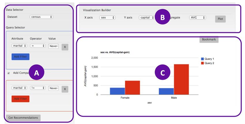
Middleware (Outside DB)
UDF-based Comparison
(w.r.t. SQL SERVER) 75 COMPARE(Our approach)
Improvement (%)
50
25
0
25
50
75 103 104 105 106 107 108
Number of Tuples
Figure 2: Relative performance of different execution approaches for a
comparative query w.r.t unmodified SQL S ERVER execution time (higher
the better). The query finds a pair of origin airports that have the most
similar departure delays over week trends in the flight dataset [1]
The complexity makes it hard for relational databases to find ef-
ficient physical plans, resulting in poor performance. While prior
work have proposed extensions [14, 13, 22, 18, 44] such as group-
ing variables, GROUPING SETS, CUBE; as we discussed in the
later sections, expressing and optimizing grouping and comparison
simultaneously remains a challenge. To describe the complexity
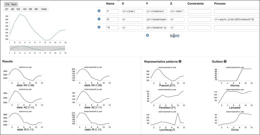
using regular SQL, we use the following example. Figure 3: A SQL query for comparing subsets of data over different at-
tribute combinations, depicting the complexity of specification using exist-
Example. Consider a market analyst exploring sales trends across
ing SQL expressions.
different cities. The analyst generates a sample of visualizations
depicting different trends, e.g., average revenue over week, aver- result for each comparison; however the join results in large inter-
age profit over week, average revenue over country, etc., for a few mediate data—one tuple for each pair of matching tuples between
cities. She notices that trends for cities in Europe look different the two sets, resulting in substantial overheads.
from those in Asia. To verify whether this observation generalizes,
she looks for a counterexample by searching for pairs of attributes 1.1 Overview of Our Approach
over which two cities in Asia and Europe have most similar trends.
Often, an Lp norm-based distance measure (e.g., Euclidean dis- In this paper, we take an important step towards making specifi-
cation of the comparative queries easier and ensuring their efficient
tance, Manhattan distance) that measures deviation between trends
and distributions is used for such comparisons [43, 47, 19]. processing. To do so, we introduce a logical operator and exten-
Figure 3 depicts a SQL query template for the above example. sions to the SQL language, as well as optimizations in relational
The query involves multiple subqueries, one for each attribute pair. databases, described below.
Within each subquery, subsets of data (one for each city) are ag- Groupwise comparison as a first class construct (Section 2 and
gregated and compared via a sequence of self-join and aggregation 3). We introduce a new logical operation, C OMPARE (Φ), as a first
functions that compute the similarity (i.e., sum of squared differ- class relational construct, and formalize its semantics that help cap-
ences). Finally, a join and filter is performed to output the tuples ture a large class of frequently used comparative queries. We pro-
of subsets with minimum scores. Clearly, the query is quite ver- pose extensions to SQL syntax that allows intuitive and more con-
bose and complex, with redundant expressions across subqueries. cise specification of comparative queries. For instance, the compar-
While comparative queries often explore and compare a large num- ison between two sets of cities C1 and C2 over n pairs of attributes:
ber of attribute pairs [47, 28], we observe that even with only a few (x1 , y1 ), (x2 , y2 ), ..., (xn , yn ) using a comparison function F can
attribute pairs, the SQL specification can become extremely long. be succinctly expressed as C OMPARE [C1 C2 ][ (x1 , y1 ), (x2 ,
Furthermore, the number of groups to compare can often be y2 ), ..., (xn , yn )] USING F. As illustrated earlier, expressing the
large—determined by the number of possible constraints (e.g., cities), same query using existing SQL clauses requires a UNION over n
pairs of attributes, and aggregation functions—which grow signifi- subqueries, one for each (xi , yi ) where each subquery itself tends
cantly with the increase in dataset size or number of attributes. This to be quite complex. Overall, while C OMPARE does not give ad-
results in many subqueries with each subquery taking substantially ditional expressive power to the relational algebra, it reduces the
long time to execute. In particular, while there are large oppor- complexity of specifying comparative queries and facilitates opti-
tunities for sharing computations (e.g., aggregations) across sub- mizations via query optimizer and the execution engine.
queries, the relational engines execute subqueries for each attribute- Efficient processing via optimizations (Section 4 and 5). We
pair separately resulting in substantial overhead in both runtime as exploit the semantics of C OMPARE to share aggregate computa-
well as storage. Furthermore, as depicted in subquery 1 in Figure tions across multiple attribute combinations, as well as partition
3, while each pair of groups (e.g., set of tuples corresponding to and compare subsets in a manner that significantly reduces the pro-
each city) can be compared independently, the relational engines cessing time. While these optimizations work for any comparison
perform an expensive self-join over a large relation consisting of function, we also introduce specific optimizations (by introducing
all groups. The cost of doing this increases super-linearly as the a new physical operator) that exploit properties of frequently used
number and size of subsets increases (discussed in more detail in comparison functions (e.g., Lp norms). These optimizations help
Section 4.1). Finally, in many cases, we only need the aggregated prune many subset comparisons without affecting the correctness.
2product =‘Inspiron’ product = ‘Inspiron’ city = ‘Tokyo’
revenue
region = ‘Asia’ city =‘Tokyo’
revenue
& region = ‘Asia’ city = ‘Paris’ city = ‘Paris’
revenue
revenue
& region = ‘Asia’
revenue
revenue
profit
region = ‘Asia’
week week week week week week category
revenue
product = ‘G7’ & region = ‘Asia’ product = ‘Inspiron’ city = ‘London’
& region = ‘Asia’ city = ‘London’ city = ‘Seoul’
revenue
region = ‘Asia’ city = ‘Beijing’
revenue
revenue
revenue
profit
profit
profit
week
week country country week week category week
product = ‘XPS’ & region = ‘Asia’ product = ‘Inspiron’
city = ‘Zurich’ city = ‘Zurich’
revenue
city =‘Beijing’
revenue
revenue
& region = ‘Asia’ city = ‘Seoul’
revenue
region = ‘Asia’
revenue
revenue
revenue
week month month week week week week
1a: One to many comparisons over fixed X and 1b: One to one comparisons over varying X and Y 2a: Many to many comparisons over fixed X and 2b: Many to many comparisons over varying
Y attributes attributes Y attributes X and Y attributes
denotes comparison
Figure 4: Illustrating comparative queries described in Section 2.1
Inter-operator optimizations (Section 6). We introduce new revenue over week trend in Asia is very dissimilar (typically mea-
transformation rules that transform the logical tree containing the sured using Lp norms) to that of the Asia’s overall trend. There are
C OMPARE operator along with other relational operators into equiv- visualization systems [48, 12, 43, 28] that support similar queries.
alent logical trees that are more efficient. For instance, the at- Example 1b. In the above example, the analyst finds that the trend
tributes referred in C OMPARE may be spread across multiple ta- for product ‘Inspiron’ is different from the overall trend for the re-
bles, involving PK-FK joins between fact and dimension tables. To gion ‘Asia’. She finds it surprising and wants to see the attributes
optimize such cases, we show how we can push C OMPARE below for which trends or distributions of Inspiron and Asia deviate the
join that reduces the number of tuples to join. Similarly, we de- most. More precisely, she wants to compare ‘Inspiron’ and ‘Asia’
scribe how aggregates can be pushed below C OMPARE, how multi- over multiple pairs of attributes (e.g., average profit over country,
ple C OMPARE operators can reordered and how we can detect and average quantitysold over week, ..., average profit over week) and
translate an equivalent sub-plan expressed using existing relational select the one where they deviate the most. Such comparisons have
operators to C OMPARE. inspired features such as Explain Data[4] in Tableau and tool such
Implementation inside commercial database engine (Section 7). as SeeDB [47], Zenvisage [43], Voyager [49].
We have prototyped our techniques in Microsoft SQL S ERVER en- Example 2a. Consider another scenario: the analyst visualizes the
gine, including the physical optimizations. Our experiments show revenue trends of a few cities in Asia and in Europe, and finds that
that even over moderately-sized datasets (e.g., 10–20 GB) C OM - while most cities in Asia have increasing revenue trends, those in
PARE results in up to 4× improvement in performance relative to Europe have decreasing trends. Again, as a counterexample to this,
alternative approaches including physical plans generated by SQL she wants to find a pair of cities in these regions where this pattern
S ERVER, UDFs, and middlewares (e.g., Zenvisage, SeeDB). With does not hold, i.e., they have the most similar trends. Such tasks
the increase in the number of tuples and attributes, the performance involving search for similar pair of items are ubiquitous in data
difference grows quickly, with C OMPARE giving more than a order mining [36] and time series [35, 10, 8, 30].
of magnitude better performance. Example 2b. In the above example, the analyst finds that the out-
put pair of visualizations look different, supporting her intuition
that perhaps no two cities in Europe and Asia have similar revenue
2. CHARACTERIZING COMPARATIVE over week trends. To verify whether this observation generalizes
QUERIES when compared over other attributes, she searches for pairs of at-
In this section, we first characterize comparative queries with the tributes (similar to ones mentioned in Example 1b) for which two
help of additional examples drawn from visualization tools [19, 43, cities in Asia and Europe have most similar trends or distributions.
47] and data mining [35, 10, 8, 30]. Then, we give a formal defini- Such queries are common in tools such as Zenvisage [43], Quick-
tion that concisely captures the semantics of comparative queries. Insights [19] that support finding outlier visualizations over a large
set of attributes.
2.1 Examples In summary, the comparative queries in above examples fast-
forward the analyst to a few visualizations that depict a pattern she
We return to the example scenario discussed in introduction: a
wants to verify—thereby allowing her to skip the tedious and time-
market analyst is exploring sales trends of products with the help
consuming process of manual comparison of all possible visualiza-
of visualizations to find unusual patterns. The analyst first looks at
tions. As illustrated in Figure 4, each query involves comparisons
a small sample of visualizations, e.g., average revenue over week
between two sets of visualizations (henceforth referred as Set1 and
trends for a few regions (e.g., Asia, Europe) and for a subset of
Set2) to find the ones which are similar or dissimilar. Each visu-
cities and products within each region. She observes some unusual
alization depicting a trend is represented via two attributes (X at-
patterns and wants to quickly find additional visualizations that ei-
tribute, e.g., week and a Y attribute, e.g., average revenue) and a set
ther support or disprove those patterns (without examining all pos-
of tuples (specified via a constraint, e.g., product = ‘Inspiron’). We
sible visualizations). Note that we use the term "trend" to refer to
now present a succinct representation to capture these semantics.
a set of tuples in a more general sense where both categorical (e.g.,
country) or ordinal attributes (e.g., week) can be used for alignment
for comparison. We consider several examples below in increasing 2.2 Formalization
order of complexity. Figure 4 illustrates each of these examples, We formalize our notion of comparative queries and propose a
depicting the differences in how the comparison is performed. concise representation for specifying such queries.
Example 1a. The analyst notes that the average revenue over week
trends for Asia as well as for a subset of products in that region look
similar. As a counterexample, she wants to find a product whose 2.2.1 Trend
3A trend is a set of tuples that are compared together as one unit. Definition 6 [Scorer]. Given two trends t1 and t2 , a scorer is any
Formally, function that returns a single scalar value called ‘score’ measuring
how t1 compares with t2 .
Definition 1 [Trend]. Given a relation R, a trend t is a set of tuples
derived from R via the triplet: constraint c, grouping g, measure m While we can accept any function that satisfies the above defi-
and represented as (c)(g, m). nition as a scorer; as mentioned earlier, two trends are often com-
pared using distance measures such as Euclidean distance, Manhat-
Definition 2 [Constraint]. Given a relation R, a constraint is a con- tan distance [31, 47, 43]. Such functions are also called aggregated
junctive filter of the form: (p1 = α1 , p2 = α2 , ..., pn = αn ) that distance functions [34]. All aggregated distance functions use a
selects a subset of tuples from R. Here, p1 , p2 , ..., pn are attributes function DIFF(.) as defined below.
in R and αi is a value of pi in R. One can use ‘ALL’ to select all
values of pi , similar to [22]. Definition 7 [DIFF(m1 , m2, p)]. 1 Given a tuple with measure value
m1 and grouping value gi in trend t1 and another tuple with mea-
Definition 3 [(Grouping, Measure)]. Given a set of tuples selected sure value m2 and the same grouping value gi , DIFF(m1 , m2 , p)
via a constraint, all tuples with the same value of grouping are = |m1 − m2 |p where p ∈ Z+ . Tuples with non-matching grouping
aggregated using measure. A tuple in one trend is only compared values are ignored.
with the tuple in another trend with the same value of grouping.
Since m1 and m2 are clear from the definition of t1 and t2 and
In example 1a, (R.region = ‘Asia’)(R.week, AVG(R.revenue)) is tuples across trends are compared only when they have same group-
a trend in Set1, where (region = ‘Asia’) is a constraint for the trend ing and measure expressions, we succinctly represent
and all tuples with the same value of grouping:‘week’ are aggre- DIFF(m1 , m2 , p) = DIFF(p)
gated using the measure: ‘AVG(revenue)’. We currently do not
Definition 8 [Aggregated Distance Function]. An aggregated dis-
support range filters for constraint.
tance function compares trends t1 : (ci )(gi , mi ) and t2 : (cj )
2.2.2 Trendset (gi , mi ) in two steps: (i) first DIFF(p) is computed between every
pairs of tuples in t1 and t2 with same values of gi , and (ii) all values
A comparative query involves two sets of trends. We formalize of DIFF(p) are aggregated using an aggregate function AGG such
this via trendset. as SUM, AVG, MIN, and MAX to return a score. An aggregated
distance function is represented as AGG OVER DIFF(p).
Definition 4 [Trendset]. A trendset is a set of trends. A trend in one
trendset is compared with a trend in another trendset. For example, Lp norms2 such as Euclidean distance can be spec-
ified using SUM OVER DIFF(2), Manhattan distance using SUM
In example 1a, the first trendset consists of a single trend: (R.region OVER DIFF(1), Mean Absolute Deviation as AVG OVER DIFF(1),
= ‘Asia’)(R.week, AVG(R.revenue))}, while the second trendset Mean Square Deviation as AVG OVER DIFF(2).
consists of as many trends as there are are unique products in R:
{(R.region = ‘Asia’, R.product = ‘Inspiron’) (R.week, AVG(R.revenue)), 2.2.4 Comparison between Trendsets
(R.region = ‘Asia’, R.product = ‘XPS’)(R.week, AVG(R.revenue)), We extend Definition 5 to the following observation over trend-
..., (R.region = ‘Asia’, R.product = ‘G7’) (R.week, AVG( R.revenue))}. sets.
As is the case in the above example, often a trendset contains one
trend for each unique value of an attribute (say p) as a constraint, Observation 1 [Comparability between two trendsets] Given two
all sharing the same (grouping, measure). Such a trendset can be trendsets T1 and T2 , a trend (ci )(gi , mi ) in T1 is compared with
succinctly represented using only the attribute name as constraint, only those trends (cj )(gj , mj ) in T2 where gi = gj and mi = mj .
i.e., [p][(g1 , m1 )]. If α1 , α2 , ..αn represent all unique values of p, Thus, given two trendsets, we can automatically infer which trends
then, between the two trendsets need to be compared. We use T 1T 2
[p][(g1 , m1 )] ⇒ {(p = α1 )(g1 , m1 ), (p = α2 )(g1 , m1 ), ..., to denote the comparison between two trendsets T1 and T2 . For
(p = αn )(g1 , m1 )} (⇒ denotes equivalence) example, the comparison in example 1a can be represented as:
Similarly, [p1 , p2 = β][(g1 , m1 )] ⇒ {(p1 = α1 , p2 = β)(g1 , [region = ‘Inspiron’][(week, AVG(revenue))] [region = ‘Asia’,
m1 ), (p1 = α2 , p2 = β)(g1 , m1 ), ..., (p1 = αn , p2 = β)(g1 , m1 )} product][ (week, AVG (revenue))]
Alternatively, a trendset consisting of different (grouping, mea- If both T1 and T2 consist of the same set of grouping and mea-
sure) combinations but the same constraint (e.g., p = α1 ) can be sure expressions say {(g1 , m1 ), ..., (gn , mn )} and differ only in
succinctly written as: constraint, we can succinctly represent T1 T2 as follows:
[(p = α1 )][(g1 , m1 ), ..., (gn , mn )] ⇒ {(p = α1 )(g1 , m1 ), ..., [c1 ][(g1 , m1 ), ..., (gn , mn )] [c2 ][(g1 , m1 ), ..., (gn , mn )] ⇒
(p = α1 )(gn , mn )} [c1 c2 ][(g1 , m1 ), ..., (gn , mn )]
Thus, the comparison between trendsets in example 1a can be
2.2.3 Scoring succinctly expressed as:
[(region = ‘Asia’) (region = ‘Asia’, product) ][(week, AVG(revenue))]
We first define our notion of ‘Comparability’ that tells when two
trends can be compared. Similarly, the following expression represents the comparison in
example 1b.
Definition 5 [Comparability of two trends]. Two trends t1 : (c1 )(g1 , [(region = ‘Asia’) (region = ‘Asia’, product = ‘Inspiron’)][(week,
m1 ) and t2 : (c1 )(g2 , m2 ) can be compared if g1 = g2 and m1 = AVG(revenue)), (country, AVG(profit)), ... , (month, AVG(revenue))]
m2 , i.e., they have the same grouping and measure. We can now define a comparative expression using the notions
For example, a trend (R.product = ‘Inspiron’) (R.week, AVG( introduced so far.
R.revenue)) and a trend (R.product = ‘XPS’)( R.month, AVG(R.profit)) 1
Note that DIFF is distinct from another operator [6] with similar
cannot be compared since they differ on grouping and measure. name.
2
Next, we define a function scorer for comparing two trends. We ignore the pth root as it does not affect the ranking of subsets.
4Table 1: Output of C OMPARE in Example 1a Table 2: Output of C OMPARE in Example 1b
R1 P W C M V O score
R1 P W V score Asia Inspiron True False False True False 40
Asia Inspiron False True False True False 20
Asia XPS True True 30 ... ... ... ... ... ... ... ...
Asia Inspiron False False True True False 10
Asia Inspiron True True 24
... ... ... ... ... Table 1 illustrate the output of this query. The first two columns
Asia G8 True True 45 R1 and P identify the values of constraint for compared trends in
T1 and T2. The columns W and V are Boolean valued denoting
whether R.week and AVG(R.revenue) were used for the compared
trends. Thus, the values of (R1, P, W, V) together identify the pairs
Definition 9 [Comparative expression]. Given two trendsets T1
of trends that are compared. Since R.week and AVG(R.revenue)
T2 over a relation R, and a scorer F, a comparative expression
are grouping and measure for all trends in this example, their values
computes the scores between trends (ci )(gi , mi ) in T1 and (cj )
are always True. Finally, the column score specifies the scores com-
(gj , mj ) in T2 where gi = gj and mi = mj .
puted using Euclidean distance, expressed as SUM OVER DIFF(2).
Now, consider below the query for example 1b that compares
3. THE COMPARE OPERATOR tuples where (R.region = Asia) with tuples where (R.region = Asia)
In this section, we introduce a new operator C OMPARE, that and (R.product = ’Inspiron’) over a set of (grouping, measure):
makes it easier for data analysts and application developers to ex-
press comparative queries. We first explain the syntax and seman- Listing 2: COMPAREXPR1B
tics of C OMPARE and then show how C OMPARE inter-operates SELECT R1, P, W, C, V, ..., M, score
with other relational operators to express top-k comparative queries FROM sales R
as discussed in Section 2.1. COMPARE [((R.region = Asia) AS R1) (R1, (R.product = ’Inspiron’)
AS P)][(R.week AS W, AVG(R.revenue) AS V), (R.country AS
3.1 Syntax and Semantics C, AVG(R.profit) AS O), ..., (R.month AS M, V)]
USING SUM OVER DIFF(2) AS score
C OMPARE, denoted by Φ, is a logical operator that takes as input
a a comparative expression specifying two trendsets T1 T2 over
relation R along with a scorer F and returns a relation R0 . Table 2 depicts the output for this query. The columns R1 and P
Φ(R, T1 T2 , F) → R0 are always set to "Asia" and "Inspiron" since the constraint for all
0
R consists of scores for each pair of compared trends between trends in T1 and T2 are fixed. W, C, M, V, and P consist of Boolean
the two trendsets. For instance, the table below depicts the out- values telling which columns among R.week, R.country, R.month,
put schema (with an example tuple) for the C OMPARE expression AVG(R.revenue), and AVG(R.profit) were used as (grouping, mea-
[c1 c2 ][(g1 , m1 ), (g2 , m2 )]. The values in the tuple indicate sure) for the pair of compared trends.
that the trend (c1 = α1 )(g1 , m1 ) is compared with the trend (c2 = From above examples, it is easy to see that we can write queries
α2 )(g1 , m1 ) and the score is 10. with C OMPARE expression for examples 2a and 2b as follows:
c1 c2 g1 m1 g2 m2 score Listing 3: COMPAREXPR2A
α1 α2 True True False False 10 SELECT R1, C1, R2, C2, W, V, score
... ... ... ... ... ... ... FROM sales R
COMPARE [((R.Region = Asia) AS R1, (R.city) AS C1) ((R.Region
= Europe) AS R2, (R.city) AS C2)][R.week AS W,
We express the C OMPARE operator in SQL using two extensions: AVG(R.revenue) AS V]
C OMPARE, and USING: USING SUM OVER DIFF(2) AS score
COMPARE T1 T2 Listing 4: COMPAREXPR2B
USING F
SELECT R1, C1, R2, C2, W, C, V, ..., M, score
For instance, for example 1a, the comparison between the AVG(revenue) FROM sales R
over week trends for the region ‘Asia’ and each of the products in COMPARE [((R.Region = Asia) AS R1, (R.city) AS C1) ((R.Region
= Europe) AS R2, (R.city) AS C2)][(R.week AS W, AVG(R.revenue) AS
region ’Asia’ can be succinctly expressed as follows: V), (R.country AS C, AVG(R.profit) AS O), ..., (R.month AS M, V)]
USING SUM OVER DIFF(2) AS score
Listing 1: COMPAREXPR1A
SELECT R1, P, W, V, score
Note that C OMPARE is semantically equivalent to a standard
FROM sales R
COMPARE [((R.region = Asia) AS R1) (R1, R.product AS P)] relational expression consisting of multiple sub-queries involving
[R.week AS W, AVG (R.revenue) AS V] union, group-by, and join operators as illustrated in introduction.
USING SUM OVER DIFF(2) AS score As such, C OMPARE does not add to the expressiveness of relational
algebra SQL language. The purpose of C OMPARE is to provide a
Here T1 = [((R.region = Asia) AS R1)][R.week AS W, AVG succinct and more intuitive mechanism to express a large class of
(R.revenue) AS V] and T2 = [((R.region = Asia) AS R1, R.product frequently used comparative queries as shown above. For example,
AS P)][R.week AS W, AVG (R.revenue) AS V]. Observe that T1 expressing the query in Listing 2 using existing SQL clauses (see
and T2 share the same set of (grouping, measure) and the filter Figure 3) is much more verbose, requiring a complex sub-query for
predicate (R.region = Asia) in their constraints, thus it is concisely each (grouping, measure). Prior work have proposed similar suc-
expressed as [((R.region = Asia) AS R1)(R1, R.product AS cinct abstractions such as GROUPING SETs [17] and CUBE [22]
P)][R.week AS W, AVG (R.revenue) AS V]. (both widely adopted by most of the databases) and more recently
5DIFF [6], which share our overall goal that with an extended syn- The SELECT clause only outputs the values of columns for which
tax, complex analytic queries are easier to write and optimize. corresponding trends has the highest score, setting NULL for other
Furthermore, the input to C OMPARE is a relation, which can ei- columns to indicate that those columns were not part of top-1 pair
ther be a base table or an output from another logical operator (e.g., of trends. This idea of setting NULL is borrowed from prior work
join over multiple tables); similarly the output relation from C OM - on Gray et al. on computing CUBE [22]. Nevertheless, an alterna-
PARE can be an input to another logical operator or the final output. tive is to output values of all columns, and add (S.W, S.M, S.C, S.P,
Thus, C OMPARE can inter-operate with other operators. In order S.V) (as in the previous example) to the output to indicate which
to illustrate this, we discuss how we C OMPARE inter-operates with columns were part of the comparison between top-1 pair of trends.
other operators such as join, filter to select top-k trends. While
C OMPARE outputs the scores for each pair of compared trends, 4. OPTIMIZING COMPARATIVE QUERIES
comparative queries often involve selection of top-k trends based In this section, we discuss how we optimize a logical query plan
on their scores (Section 2.1). consisting of a C OMPARE operation. Microsoft SQL S ERVER uses
a cost-based optimizer for generating the physical plan for an in-
3.2 Expressing Top-k Comparative Queries put logical plan. We extend the optimizer to replace C OMPARE
In this section, we show how we can use the above-listed C OM - with a sub-plan of existing physical operators such that cost of the
PARE sub-expressions (referred by COMPAREXPR1A, COMPAR- sub-plan is least. This is done in two steps: we first transform
EXPR1B, COMPAREXPR2A, and COMPAREXPR1B) with LIMIT C OMPARE into a sub-plan of existing logical operators. These log-
and join to select tuples for trends belonging to top-k. ical operators are then transformed into physical operators using
Example 1a. The following query selects the tuples of a prod- existing rules to compute the cost of C OMPARE. The cost of the
uct in region ‘Asia’ that has the most different AVG(revenue) over sub-plan for C OMPARE is combined with costs of other physical
week trends compared to that of region ‘Asia’ overall. COMPAR- operators to estimate the total cost of the query. We state our prob-
EXPR1A refers to the sub-expression in Listing 1. lem formally:
SELECT T.product, T.week, T.revenue, S.score
FROM sales T JOIN
Problem 4.1. Given a logical query plan consisting of C OMPARE
(SELECT * FROM COMPAREXPR1A operation: Φ(R, [c1 c2 ] [(d1 , m1 ), ..., (dn , mn )], F) → R0 ,
ORDER BY score DESC replace C OMPARE with a sub-plan of physical operators with the
LIMIT 1) AS S lowest cost.
WHERE T.product = S.P
For ease of exposition, we assume that both trendsets contain the
The ORDER BY and LIMIT clause select the top-1 row in Ta- same set of trends, one for each unique value of c, i.e., c1 = c2 = c.
ble 1 with the highest score with P consisting of the most similar
product. Next, a join is performed with the base table to select all 4.1 Basic Execution
tuples of the most similar product along with its score. We start with a simple approach that transforms C OMPARE into
Example 2a. The query for example 2a differs from example 1a a sub-plan of logical operators. The sub-plan is similar to the one
in that both trendsets consist of multiple trends. Here, one may be generated by database engines when comparative queries are ex-
interested in selecting tuples of both cities that are similar, thus we pressed using existing SQL clauses (discussed in Section 1). We
use the WHERE condition (T.city = S.C1 AND T.Region = S.R1) perform the transformation using the following steps, with each
OR (T.city = S.C2 AND T.Region = S.R2). (S.R1, S.R2, S.C1, step using the output from previous step as input.
S.C2) in SELECT clause identifies the pair of compared trends. (1) ∀(di , mi ): Ri ← Group-byc,di Aggmi (R)
(2) ∀ Ri : Rij ←1Ri .c!=Ri .c,Ri .di =Ri .di (Ri )
SELECT T.Region, T.city, T.week, T.revenue, S.R1, S.C1, S.R2, S.C2, (3) ∀ Rij : Rijk ← Group-byci ,cj AggUDAF (Rij ) // ci , cj are
S.score
aliases of column c
FROM sales T JOIN
(SELECT * FROM COMPAREXPR2A (4) R0 ← Union All(Rijk )
i,j,k
ORDER BY score First, for each (grouping, measure) combination, we add a group-
LIMIT 1) AS S
by aggregate (e.g., GROUP BY product, week, AGG on AVG(revenue))
WHERE (T.city = S.C1 AND T.Region = S.R1) OR (T.city = S.C2 AND
T.Region = S.R2) to create trendsets. Then, on the output of group-by aggregate, we
join tuples between two trends that have the same value of grouping
(e.g., 1R’.product !=R’.product, R’.week = R’.week )). Finally, the score between
Examples 1b and 2b. These examples extend the first two exam- each pair of trends is computed by applying a user-defined aggre-
ples to multiple attributes. We show the query for example 2b; it’s gate (UDA) F. This is done by first partitioning the join output
a complex version of (example 1b) where trends in each trendsets to group together each pair of trends. Each partition consisting of
are created by varying all three: constraint, grouping, measure (ex- pair of trends is then aggregated using F. Finally, the scores for all
ample 1b has a fixed constraint for each trendset). pairs of trends are aggregated via Union All.
SELECT T.city, S.R1, S.R2, S.C1, S.C2, Unfortunately, this approach does not scale well as the size of
CASE WHEN S.W THEN T.week ELSE NULL END, the input dataset and the number of (grouping, measure) combi-
... nations become large. There are two issues. First, aggregations
CASE WHEN S.V THEN T.revenue ELSE NULL END, across (grouping, measure) are performed separately, even when
S.score
there are overlaps in the subset of tuples being aggregated. Second,
FROM sales T JOIN
(SELECT * FROM COMPAREXPR2B while each trend is compared with other trends independently, the
ORDER BY score second step typically involves a join at the granularity of trendsets,
LIMIT 1) AS S i.e., a relation consisting of one trendset is joined with a relation
WHERE (T.city = S.C1 AND T.Region = S.R1) OR (T.city = S.C2 AND consisting of another trendset. The cost of join increases rapidly
T.Region = S.R2) as the number of trends being compared and the size of each trend
63. Trend-wise UNION ALL
comparison
......
...... ...... ......
......
Latency (s)50 ⨝ ⨝ ......⨝ ⨝
......⨝ ......⨝ ......⨝
......⨝
....
Grp-by {c1d1} Grp-by {c2d1}
.... Grp-by {cnd1} ......... ......... .........
25 Agg on {m1} Agg on {m1} Agg on {m1} .........
Partition Partition
Partition ......... .........
on c on c
on c
cd6m6 cd4m4
cd1m1
20 18 16 14 12 10 8 6 4 21
Partition
Horizontal
Vertical
Partition
on (dimi)
.........
Partitioning on (dimi)
Number of group-by expressions
Partitioning
2. Partitioning .........
after merging TrendSet into
Trends 1. Merging
Group-by {c d1d6d4}
Aggregate on {m1m6m4}
Group-by {c d2dn}
Aggregate on {m2mn}
.........
aggregates
(a) Variation in performance as we merge group-by ag- R
gregates to share computations Figure 6: Optimized query plan generated after applying merging and par-
Trendsetwise Join
titioning on basic query plan in Figure 7.
300 Partitioning + Trendwise Join
Latency (s)
impact of merging on the cost of subsequent comparison between
200 Only Partitioning trends; ignoring which can lead to sub-optimal plans as we describe
100 shortly. We first introduce the second optimization for comparison.
Trendwise Comparison via Partitioning. The second optimiza-
101 102 103 104 105 tion is based on the observation that pairwise joins of multiple
Number of trends per trendset smaller relations is much faster than the a single join between two
large relations. This is because the cost of join increases super-
(b) Improvements due to trendwise join after partition- linearly with the increase in the size of the trendsets. In addi-
ing trendset into trends (the size of each trend is fixed to tion to improvement in complexity, trend-wise joins are also more
1000 tuples) amenable to parallelization than a single join between two trend-
sets. Figure 5b depicts the difference in latency for these two ap-
Figure 5: Improvement in performance due to merging group-by proaches as we increase the number of trends from 10 to 105 (each
aggregates and trendwise comparison (via partitioning) of size 1000). The black dotted line shows the partitioning over-
head incurred while creating partitions for each trend, showing that
the overhead is small (linear in n) compared to the gains due to
increases (see Figure 5b). We next discuss how we address these trendwise join. Moreover, this is much smaller than the overhead
issues via merging and partitioning optimizations. incurred when partitioning is performed on the join output (∝ n2 )
in the basic plan (see step 3 in Figure 5).
4.2 Merging and Partitioning Optimization Figure 7 depicts the query plan after applying the above two op-
To generate a more efficient plan, we adapt the sub-plan gener- timizations on the basic query plan. First,we merge multiple group-
ated above using two steps. First, we merge group-by aggregates by aggregates to share computations (using the approach discussed
into a fewer number of group-by aggregates. Next, we partition below). Then, we partition the output of merged group-by aggre-
the output of group-by aggregates to create one relation for each gates into smaller relations, one for each trend. This is followed
trend, which allows parallel join and comparison for scoring. We by joining and scoring between each pair of trends independently
describe each of these optimizations and then present an algorithm and in parallel. Observe that the merging of group-by aggregates
that jointly optimizes them to find an overall efficient plan. results in multiple trends with overlapping (grouping, measure) in
Merging group-by aggregates. The first optimization shares the the output relation. Hence, we apply the partitioning in two phases.
computations across a set of group-by aggregates, one for each In the first phase, we partition it vertically, creating one relation
(grouping, measure), by merging them into fewer group-by aggre- for each (grouping, measure). In the second phase, we partition
gates. Many (grouping, measure) often share a common group- horizontally, creating one relation for each trend.
ing column, e.g., [(day, AVG(revenue), (day, AVG(profit)] or have Joint Optimization of Merging and Partitioning. As depicted in
correlated grouping columns (e.g., [(day, AVG(revenue), (month, Figure 6b, the cost of partitioning increases with the increase in the
AVG(revenue)]) with high degree of overlapping tuples across trends. size of its input. The input size is proportional to the number of
To illustrate, we considered a set of 20 group-by aggregates in the unique group-by values, which increases with the increase in the
flights [1] dataset, computing avg(ArrivalDelay), avg(DepDelay), number of merging of group-by aggregates. Thus, when the input
..., avg(Duration) grouped by day, week, ..., airport. As depicted in becomes large, the cost of partitioning dominates the gains due to
Figure 5a, by merging them (using an approach discussed shortly) merging. It is therefore important to merge group-by aggregates
into 12 aggregates, the latency improves by 2×. Furthermore, we such that the overall cost of computing group-by aggregates, parti-
can see that after a certain number of merges, the performance de- tioning and trendwise comparison together is minimal.
grades. This is because the sharing of tuples decreases as we merge In order to find the optimal merging and partitioning, we follow
additional grouping columns, which in turn results in the larger in- a greedy approach as outlined in Algorithm 1. Our key idea is to
crease in the output size of group-by aggregates. merge at the granularity of sub-plans instead of the group-by ag-
Finding the optimal merging of group-by aggregates is NP- Com- gregates. We start with a set of sub-plans, one for each (grouping,
plete [7]. Prior work on optimizing GROUPING SETS compu- measure) as generated by the basic execution strategy discussed
tation [17] have proposed best-first greedy approaches that merge earlier and merge two sub-plan at a time that lead to the maximum
those group-by aggregates first that lead to maximum decrease in decrease in cost.
the cost. Unfortunately, in our setting, we also need to consider the Formally, if the two sub-plans operate over (d1 , m1 ) and (d2 ,
7m2 ) respectively, we merge them using the following steps (illus- the two trends as we discuss below. Given the upper and lower
trated in Figure 6): bound scores of each pair, we find a pruning threshold T on the
(1) R1 ← Group-byc,d1 ,d2 Aggm2 ,m2 [R] // merge group-by aggre- lowest possible top k score, as the kth largest lower bound score
gates across all pairs . Any pair with its upper bound score smaller than
(2) ∀ (di , mi ): Ri ← Π(di ,mi ) (R1) // vertical partitioning T can thus be pruned. 3. Finally, we perform a join between the
(3) ∀ i: Rij ← Partition Ri ON c // horizontal partitioning, one tuples of trends that are not pruned.
partition for each value of c
[28, 30] [15, 19] [26, 29] [28, 30] [26, 29]
(4) ∀ i, j: Ri0 j 0 ← Group-bycj ,di Aggmi [Rij ] // aggregate again 3
⨝ ⨝ ⨝ ⨝ ⨝
(5) ∀ i0 , j 0 , k: Ri0 j 0 k ← Ri0 j 0 1di Ri0 k //partitition-wise join 2
0
(6) ∀ i0 , j 0 , k: Ri0 j 0 k ← AggUDAF (Ri0 j 0 k ) // compute scores Bitmap +
Summary
Bitmap +
Summary
Bitmap +
Summary
0 Aggregates Aggregates Aggregates
0
(7) R ← Union
0 0
All(Ri0 j 0 k ) 1
i ,j ,k
P1 P2 P3 P1 P2 P3
We first merge group-by aggregates, followed by creating one
partitions for each trend using both vertical and horizontal par- Figure 7: Illustrating pruning for DIFF-based comparisons
titioning. Then, we join pairs of trends and compute the score. We empirically show in Section 8 that while the pruning incurs
For computing the cost of the merged sub-plan, we use the opti- an overhead of first computing the summary aggregates and bitmap
mizer cost model. The cost is computed as a function of avail- for each candidate trend, the gains from skipping tuple comparisons
able database statistics (e.g., histograms, distinct value estimates), for pruned trends offsets the overhead. Moreover, the summary
which also captures the effects of the current physical design, e.g., aggregates of each trend can be computed independently in parallel.
indexes as well as degree of parallelism (DOP). We merge two sub Computing Bounds. The simplest approach is to create a sin-
plans at a time until there is no improvement in cost. gle set of summary aggregates for each trend as depicted in Fig-
ure 8b. The gray and yellow blocks depict the summary aggregates
for two trends respectively, consisting of COUNT (computed using
Algorithm 1 Merge-Partition Algorithm
bitmaps), SUM, MIN, and MAX in order.
1: Let B be a basic sub-plan computed from Φ as described in Section 4.1 First, for deriving the lower bound, we prove the following useful
2: while true do
3: C ← OptimizerCost(B)
property based on the convexity property of DIFF functions (see
4: Let si ∈ S be a sub-plan in B consisting of a sequence of group-by [2] for the proof).
aggregate, join and partition operations over (di , mi )
5: Let M P = Set of all sub-plans obtained by merging a pair of sub-
Theorem 1. ∀ DIFF(m1 , m2 , p),
plans in S as described in Section 4.2 AVG (DIFF(m1 , m2 , p)) ≥ DIFF(AVG (m1 ),AVG (m2 ), p)
6: Let Bnew be the sub-plan in M P with lowest cost (Cnew ) after This essentially allows us to apply DIFF on the average values
merging two sub-plans si , sj of each trend to get a sufficiently tight lower bounds on scores. For
7: if Cnew > C then
example, in Figure 8b, we get a lower bound of 1700 for a score of
8: break;
9: end if 1717 for the two trends shown in Figure 8b.
10: C ← Cnew For the upper bound, it is easy to see that the maximum value
11: B ← Bnew of DIFF(m1 , m2 , 2) between any pairs of tuples in R and S is
12: end while given by: MAX ( |MAX (m1 ) − MIN (m2 )|, |MAX (m2 ) − MIN
13: Return B (m1 )|). Given that DIFF(m1 , m2 , 2) is Non-negative and Mono-
tonic, we can compute the upper bound on SUM by multiplying
the the MAX (DIFF(m1 , m2 , 2)) by COUNT. For example, in Fig-
5. OPTIMIZING DIFF-BASED COMPARI- ure 8b, we get an upper bound of 6400.
SON Multiple Piecewise Summaries. Given that the value of measure
While the approach discussed in the previous section works for can vary over a wide range in each trend, using a single sum-
any arbitrary scorer, we note that for top-k comparative queries in- mary aggregate often does not result in tight upper bound. Thus,
volving aggregated distance functions (defined in Section 2.2) such to tighten the upper bounds, we create multiple summary aggre-
as Euclidean distance, we can substantially reduce the cost of com- gates for each trend, by logically dividing each trend into a se-
parison between pairs of trends. We first outline the three properties quence of l segments, where segment i represents tuples from in-
of DIFF(.) function that we leverage for optimizations. dex: (i − 1) × nl + 1 to i × nl where n is the number of tuples
1. Non-negativity: DIFF( m1 , m2 , p) ≥ 0 in the trend. Instead of creating a single summary, we compute
the set of same summary aggregates over each segment, called seg-
2. Monotonicity: DIFF(m1 , m2 , p) varies monotonically with the
ment aggregates. For example, Figure 8c depicts two segment ag-
increase or decrease in |m1 − m2 |.
gregates for each trend, with each segment representing a range
3. Convexity: DIFF( m1 , m2 , p) are convex for all p. of 8 tuples. The bounds between a pair of matching segments is
computed in the same way as we described above for a single sum-
5.1 Summarize → Bound → Prune mary aggregates. Then, we sum over the bounds across all pairs
Overview. We introduce a new physical operator that minimizes of matching segments to get the overall bound (see [2] for formal
the number of trends that are compared using the following three description). As we can see in Figure 8c, increasing the number of
steps (illustrated in Figure 8). 1. We summarize each trend inde- segments from 1 to 2 improves the bounds from [1700, 6400] to
pendently using a set of three aggregates: SUM, MIN and MAX [1702, 4624], substantially reducing the upper bound.
and a bitmap corresponding to the grouping column. 2. Next, we To estimate the number of summary aggregates for each trend,
intersect the bitmaps between trends to compute the COUNT of we use Sturges formula, i.e., (b1 + log2 (n)c) [42], which assumes
matching tuples between them. We use the COUNT along with the normal distribution of measure values for each trend. Because
three aggregates to compute the upper and lower bounds between of its low computation overhead and effectiveness in capturing the
818 18 14 18 18 16 14 14 10 14 12 10 13 13 14 14 16, 229, 10, 18 8, 129, 13, 18 8, 100, 10, 14
Score = 1717 Bounds = [1700, 6400] Bounds = [1702, 4624]
26 23 23 29 30 28 24 25 27 24 24 20 21 25 20 22 16, 394, 20, 30 8, 211, 23, 30 8, 183, 20, 27
(b) Bounds on score us- (c) Bounds on score using
(a) Exact score on comparing two trends
ing a single summary two-segment summaries
Figure 8: Using summaries to bound scores. F = SUM OVER DIFF(2). Each value in (a) corresponds to a single tuple in a trend.
distribution or trends of values, Sturges formula is widely used in Algorithm 2 Pruning Algorithm for DIFF-based Comparison
the statistical packages for automatically segmenting or binning 1: Compute SegAgg and bitmaps for each candidate trend ci
data points into fewer groups. We empirically show in Section 8 2: for each pair of trends ci , cj do
(see Figure 11a) that (b1 + log2 (n)c) number of segments per trend 3: Compute bounds on scores (Section 5.1)
results in sufficiently tight bounds for effective pruning, without 4: Update PQS
5: end for
adding significant computational overhead. 6: for each candidate trend ci do
7: If ((ci , cj ) upper bound < PQS .Top()) Continue;
5.2 Early Termination 8: Initialize (ci , cj ) TState and push to PQP
For early termination of the top-k trends search among the un- 9: end for
10: while size of PQP > k do
pruned trends, we assign an utility to each of the unpruned trends 11: (ci , cj ) = PQP .Top()
that tells how likely they are going to be in the top-k. 12: Compare a segment ci , with that of cj
For estimating the utility of trends , we use the bounds computed 13: Update bounds and PQS
using segment aggregates in the previous step. Specifically, for se- 14: If ((ci , cj ) upper bound < PQS .Top()) Continue;
lecting top-k trends in descending order of their scores, a trend with 15: Push (ci , cj ) to PQP
higher upper bound score has a higher utility. On the other hand, 16: end while
17: Return Top k trend pairs from PQP
for top-k trends in ascending order of their scores, a trend with the
smallest lower bound has a higher utility. The processing of higher
utility trends leads to the faster improvement in the pruning thresh-
fetch the trend with the highest upper bound score ((line 11)), and
old T, thereby minimizing wastage of tuple comparisons over low
following the process outlined in Section 5.2, compare one of its
utility trends.
segments with a segment from the reference trend (line 12). After
Moreover, the utility of a trend can increase or decrease after
processing a segment, we check if the current trend pair is pruned or
comparing a few tuples in a candidate trend. Hence, instead of
if there is another trend pair with higher upper bound (line 14–15).
processing the entire trend in one go, we process one segment of
This process is continued until we are left with k pairs of trends .
a trend at a time, and then updates the bounds to check (i) if the
Finally, we output values of k pairs of trends with highest scores
trend can be pruned, or (ii) if there is another trend with better
(line 17).
upper bounds that it should switch to. As we show in Section 8,
incrementally comparing high utility trends first leads to pruning Memory Overhead. Given a relation of n tuples consisting of
of many trends without processing all of their tuples. p trends, Φp creates p × log(n/p) segment aggregates, each seg-
ment aggregate consisting of 4 aggregates values. In addition, the
5.3 Putting It All Together operator maintains a TState consisting of a fixed number of ele-
In order to support the above optimizations, we implemented a ments per trend, including the largest k lower bounds on scores.
new physical operator, Φp , that takes as input the partitions (one for Thus, the overall space overhead is O(p × log(n/p)) + 10 × p
each trend), and replaces the join and F in query plans discussed + k) ≈ O(p × log(n/p)). Thus, for an input relation, consist-
in Section 4. It outputs a relation consisting of tuples that identify ing of 100 million tuples with 100 trends and 3 attributes, of total
the top-k pairs of trends as discussed in Section 3. The algorithm size about 2.5 GB, Φp incurs an overhead of approximately 64K
used by the operator makes use of four data structures: (1) SegAgg floating point numbers (< 1 MB).
: An array where index i stores summary aggregates for segment
i. There is one SegAgg per trend. (2) TState : The state of a trend,
6. ADDITIONAL ALGEBRAIC RULES
consisting of the current upper and lowers bounds on the score, The query optimizer in Microsoft SQL S ERVER relies on alge-
as well as the next segment within the trend to be compared next. braic equivalence rules for enumerating query plans to find the plan
There is one TState for each trend, and is updated after comparing with the least cost. When C OMPARE occurs with other logical oper-
each segment. (3) PQP : a MAX priority queue that keeps track ators, we present five transformation rules (see Table 3) that reorder
of the trend pairs with the highest upper bound. It is updated after Φ with other operators to generate more efficient plans.
comparing each segment. (4) PQS : a MIN priority queue that R1. Pushing Φ below join. Data warehouses often have a snowflake
keeps track of the trend pairs with the smallest lowest bound. It is or star schema, where the input to C OMPARE operation may involve
updated after comparing each segment. a PK-FK join between fact and dimension tables. If one or more
Algorithm 2 depicts the pseudo-code for a single threaded im- columns in Φ are the PK columns or have functional dependen-
plementation. We first compute the segment aggregates for trends cies on the PK columns in the dimension tables , Φ can be pushed
(line 1). For each pair of trends, we compute the bounds on scores down below the join on fact table by replacing the dimension tables
as discussed in Section 5.1, and update PQS to keep track of top columns with the corresponding FK columns in the fact table (see
k lower bounds (lines 2—5). The upper bound for each trend pair Rule R1 in Table 3.) For instance, consider example 1a in Section
is compared with PQS .Top() to check if it can be pruned (line 7). 2.1 that finds a product with a similar average revenue over week
If not pruned, the TState is initialized and pushed to PQP (line trend to ‘Asia’. Here, revenue column would typically be in a fact
8). Once the TState of all unpruned trends are pushed to PQP , we table along with foreign key columns for region, product and year.
9Table 3: Algebraic equivalence rules for Φ: COMPARE [P1 = α1 |P2=α2 ][(M1, M2)] USING A OVER F
Rule Equivalence rule Pre-condition
R1 Φ(R 1T S) ≡ (Φk (R)) 1T S T: PK in S; T ⊆ {P1,P2, M1, M2} ⊆ R ;Φk : Φ with PK columns replaced with FK columns
R2 ΥG,A (Φ(R)) ≡ Φ(ΥG,A (R)) {P1, P2, M1, M2} ⊆ G and A ∈ {MAX,MIN }
R3 σC (Φ(R)) ≡ Φ(σC (R)) C ⊆ {P1, P2}
R4 Φ2 (Φ1 (R)) ≡ Φ1 (Φ2 (R))) Φ1 : P1 , P2 = Φ2 : P1 , P2
R5 (LIMITK Υ(ΠDIFF(R.X, L.X, p) (σP =α R) 1 R)) 1 R ≡ Φ(R) None
In such cases, we can push Φ below the join by replacing dimen- DIFF-based comparisons can be further optimized by adding a new
sion table columns (e.g., product, week) values with corresponding physical operator that first computes the upper and lower bounds on
PK column values. the scores of each trend, which can then be used for pruning parti-
R2. Pushing Group-by Aggregate (Υ) below Φ to remove du- tions without performing costly join.
plicates. When an aggregate operation occurs above a C OMPARE Robustness to physical design changes. A large part of C OM -
operation, in some cases we can push the aggregate operation be- PARE execution involves operators such as group-by, joins and par-
low the C OMPARE to reduce the size of each partition. In particular, tition (See Figure 6). Hence, the effect of physical design changes
consider an aggregate operation ΥG,A with group by attributes G on C OMPARE is similar to their effect on these operators. For in-
and aggregate function A such that all columns used in Φ are in G. stance, since column-stores tend to improve the performance of
Then, if all aggregation functions in Φ ∈ {MAX, MIN }, we can group-by operations, they will likely improve the performance of
push Υ below Φ as per the Rule R2 in Table 3. Pushing aggregation C OMPARE. Similarly, if indexes are ordered on the columns used
operation below Φ reduces the size of each partition by removing in constraints or grouping, the optimizer will pick merge join over
the duplicate values. hash-join for joining tuples from two trends. Finally, if there is a
R3. Predicate pushdown. A filter operation (σ) on partition col- materialized view for a part of the C OMPARE expression, modern
umn (e.g., product) can be pushed down below Φ, to reduce the day optimizers can match and replace the part of the sub-plan with
number of partitions to be compared. While predicate pushdown in a scan over the materialized view. We empirically evaluate the im-
a standard optimization, we notice that optimizers are unable to ap- pact of indexes on C OMPARE implementation in Section 8.
ply such optimizations when the C OMPARE are expressed via com- Applications of C OMPARE. C OMPARE is meant to be used by
plex combination of operations as described in Section 1. Adding data analysts as well as applications to issue comparative queries
an explicit logical C OMPARE, with a predicate pushdown rule makes over large datasets stored in relational databases. It has two advan-
it easier for the optimizer to apply this optimization. Note that if σ tages over regular SQL and middleware approaches (e.g., Zenvis-
involves any attribute other than the partitioning column, then we age, Seedb). First, it allows succinct specification of comparative
cannot push it below Φ. This is because the number of tuples for queries which can be invoked from data analytic tools supporting
partitions compared in Φ can vary depending on its location. SQL clients. Second, it helps avoid data movement and serializa-
R4. Commutativity. Finally, a single query can consist of a chain tion and deserialization overheads, and is thus more efficient and
of multiple C OMPARE operations for performing comparison based scalable. We classify the applications into three categories:
on different metrics (e.g., comparing products first on revenue, and BI Tools. BI applications such as Tableau and Power BI do not pro-
then on profit). When multiple Φ operations on the same parti- vide an easier mechanism for analysts to compare visualizations.
tioning attribute, we can swap the order such that more selective However, for supporting complex analytics involving multiple joins
C OMPARE operation is executed first. and sub-queries, these tools support SQL querying interfaces. For
R5. Reducing comparative sub-plans to Φ. Finally, we extend comparative queries, users currently have to either write complex
the optimizer to check for an occurrence of the comparative sub- SQL queries as discussed in Introduction, or generate all possible
expression specified using existing relational operators to create an visualizations and compare them manually. With C OMPARE, users
alternative candidate plan by replacing the sub-expression with Φ. can now succinctly express such queries (as illustrated in Section
In order to do so, we add the equivalence rule R5 where the expres- 3) for in-database comparison.
sion on the left side represents the sub-expression using existing Notebooks. For large datasets stored in relational databases, it is
relational operators. This rule allows us to leverage physical op- inefficient to pull the data into notebook and use dataframe APIs
timizations for comparative queries expressed without using SQL for processing. Hence, analysts often use a SQL interface to access
extensions. and manipulate data within databases. While one can also expose
Python APIs for comparative queries and automatically translate
them to SQL, such features are limited to the users of the Python
7. DISCUSSION library. SQL extensions, on the other hand, can be invoked from
We discuss the generalizability and robustness of our proposed multiple applications and languages that support SQL clients. Fur-
optimizations as well as potential applications of C OMPARE. thermore, in the same query, one can use C OMPARE along with
Generalizability of optimizations. Our proposed optimizations in other relational operators such as join and group-by that are fre-
Section 4 deal with replacing C OMPARE to a sub-plan of logical quently used in data analytics (see Section 3.2).
and physical operators within existing database engines. These op- Visual analytic tools. Finally, there are visual analytic tools such as
timizations can be incorporated in other database engines support- as Zenvisage and Seedb that perform comparison between subsets
ing cost-based optimizations and addition of new transformation of data in a middle-ware. With C OMPARE, such tools can scale to
rules. Concretely, given a C OMPARE expression, one can generate large datasets and decrease the latency of queries as we show in
a sub-plan using Algorithm 1 and transformation rules implement- Section 8.
ing steps outlined in Section 4.1 and Section 4.2. Furthermore, we
discuss additional transformation rules (see Table 3) in Section 6
that optimize the query when C OMPARE occurs along with other
logical operators such as join, group-by, and filter. We show that 8. PERFORMANCE EVALUATION
10You can also read