Manual for Application of the European Fish Index (EFI)
←
→
Page content transcription
If your browser does not render page correctly, please read the page content below
���������������������
                                        ���������

Manual for Application
of the European Fish Index (EFI)

Development, Evaluation and Implementation of a
standardised Fish-based Assessment Method for
the Ecological Status of European Rivers (FAME)

A Contribution to the
Water Framework Directive
A research project supported by the European Commission under FP 5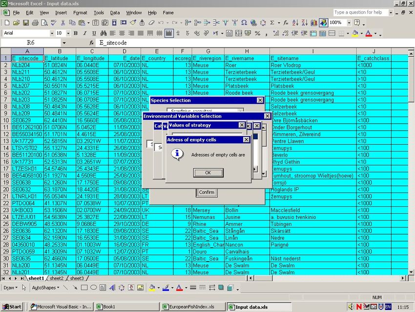
MANUAL
                      FOR THE APPLICATION
                 OF THE European Fish Index - EFI
  A FISH-BASED METHOD TO ASSESS THE ECOLOGICAL STATUS OF EUROPEAN RIVERS
               IN SUPPORT OF THE WATER FRAMEWORK DIRECTIVE

                             VERSION 1.1, January 2005
                        DEVELOPED BY THE FAME CONSORTIUM

FAME - Development, Evaluation and Implementation of a Standardised Fish-based Assessment Method for the
         Ecological Status of European Rivers. A Contribution to the Water Framework Directive
    A project under the 5th Framework Programme Energy, Environment and Sustainable Development
                      Key Action 1: Sustainable Management and Quality of Water
                                  Contract No: EVK1 -CT-2001-00094
                                         http://fame.boku.ac.at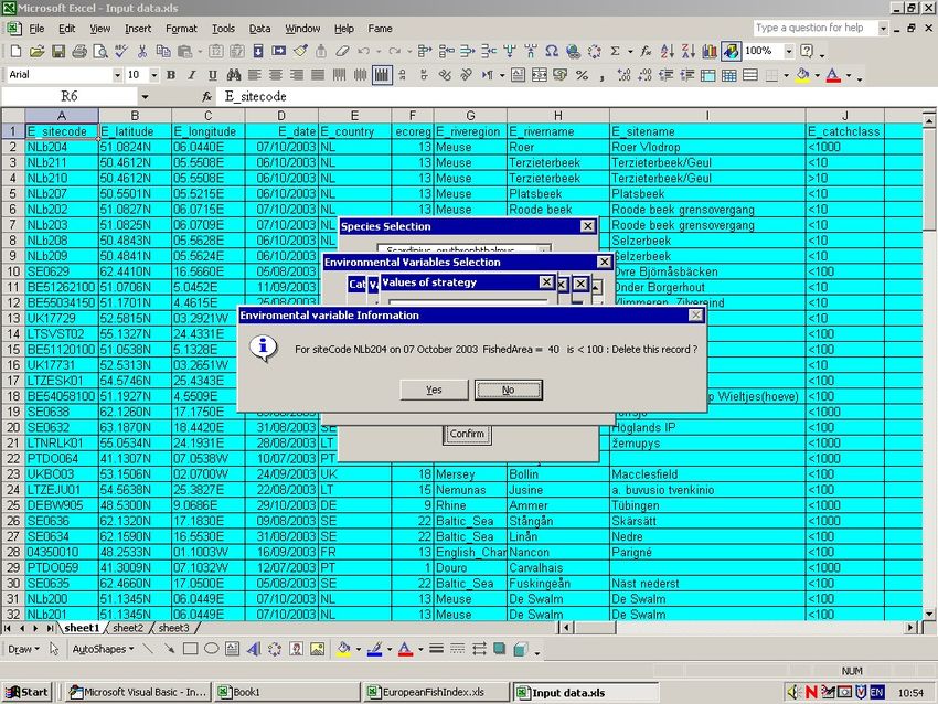
To be cited as: FAME CONSORTIUM (2004). Manual for the application of the European Fish
Index - EFI. A fish-based method to assess the ecological status of European rivers in support of
the Water Framework Directive. Version 1.1, January 2005.

The text of this manual was written by Jan Breine, Ilse Simoens, Gertrud Haidvogl, Andreas
Melcher, Didier Pont, & Stefan Schmutz.

Acknowledgements

The FAME consortium would like to thank numerous individual persons, private and public
institutions throughout Europe for providing the large volume of data that made the FAME
project possible. Special thanks are dedicated to Paul Angermeier, Virginia TECH US, and
Robert Konecny, Environmental Agency Austria, for reviewing the FAME project. We are
grateful to Richard Noble for his critical revision and valuable suggestions. The consortium
greatly appreciated the support of Hartmut Barth and Mogens Gadeberg, the Scientific Officers
of the EC.
The FAME project was financed by the EC contract no. EVK1 -CT-2001-00094.

Help desk: Please direct all questions and suggestions for improvements to fame@boku.ac.at.

Layout: Filip Coopman

Printed in 2004 by Ministerie van de Vlaamse Gemeenschap, Departement L.I.N. A.A.D. afd.
Logistiek-Digitale drukkerij
Contents
Preface                                                             6

General Introduction                                                7

Part I: Introduction                                                8
      1. The Water Framework Directive (WFD)                        8
      2. Fish-based ecological assessment methods in Europe         9
      3. What is an Index of Biotic Integrity (IBI)?                9
      4. Why fish?                                                  10
Part II: The European research project FAME                         11
      1. Introduction                                               11
      2. Basic tools of FAME used to develop the EFI                12
      3. European Fish Index EFI                                    13
      4. Limitations of the EFI                                     20
                     Example of application                         18
      5. European fish typology (EFT)                               23
      6. Collecting data for the EFI                                25
                     Site selection                                 26
                     Environmental variables and sampling methods   26
                     Fish sampling                                  26
                     Fish data                                      30
Part III: A manual for application                                  31
      1. Preparing data in MS Excel: data organization and format   31
      2. Installing the software                                    33
      3. Entering new data in the software                          41
      4. Data quality control with an example                       45
      5. Index calculation                                          57
                     Step 1                                         58
                     Step 2                                         60
      6. Defining the European Fish Type                            62
Remarks                                                             65
References                                                          66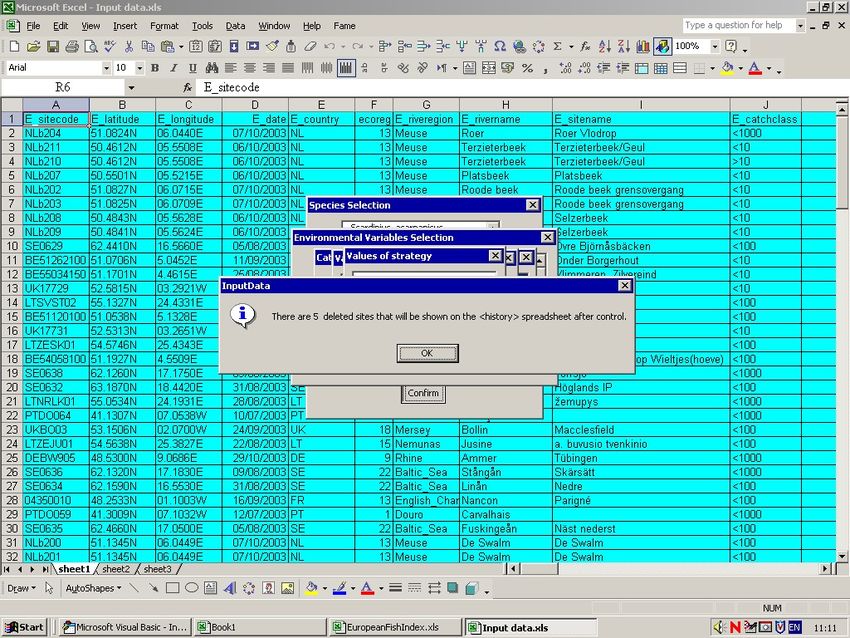
Annexes
1 Field Protocol: 3 tables
2 River groups and ecoregions: 2 figures & 2 tables
3 Fish species in EFI software
4 Guilds table: 2 tables
5 Glossary for FAME

List of figures, pictures and tables
Figure 1: Steps prescribed in the WFD for ecological status assessment             8
Figure 2: Countries participating in FAME                                          11
Figure 3: Structure of the central database, FIDES (Fish Database of European
Streams), and relations between tables                                             12
Figure 4: The methodology of the EFI. In step 3 to 6 two examples, a reference
site (green) and a disturbed site (red) are shown                                  17
Figure 5: Process of converting species data into observed metric values
- River Dropt, France                                                              19
Figure 6: Different steps required to apply the assessment method                  25

Picture 1 Electric fishing in a wadable river                                      28
Picture 2 Electric fishing from a boat                                             29

Table 1: The 10 metrics used by the EFI and their response to human pressures
(↓ = decrease; ↑ = increase of metric                                              13
Table 2: Abiotic variables and sampling method variables required for the EFI
to predict reference conditions (variable codes for the EFI software in italics)   16
Table 3: Example of site information and environmental variables - river Dropt
France                                                                             18
Table 4: Observed, theoretical and probability metric values - river Dropt,
France                                                                             20
Table 5: Minimum, median and maximal values of environmental characteristics       21
Table 6: The 15 European Fish Types and relative species composition (%), only
species >2% are listed (species >12 % in bold)                                     23
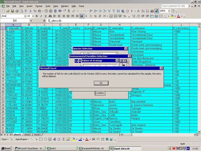
Table 7: Distribution of European fish types across ecoregions and abiotic
variables (mean values) discriminating between the 15 European Fish Types    24
Table 8: Rivers < 0.7 m depth = wadable rivers                               28
Table 9: Rivers > 0.7 m depth = non-wadable rivers (boat fishing)            29
Table 10: Metrics and abbreviations in results spreadsheet, ‘MA’ metric
abbreviations used in metrics spreadsheet. N.ha = number per hectare;
n.sp = number of species; perc.nha = percent of number per hectare;
perc.sp = percent number of species                                          59
Preface

This manual describes the European Fish Index - EFI - and its application software. The EFI
and the manual have been developed within the EU research and development project FAME
(Development, Evaluation and Implementation of a Standardised Fish-based Assessment
Method for the Ecological Status of European Rivers - A Contribution to the Water
Framework Directive). FAME was a project under the 5th Framework Programme Energy,
Environment and Sustainable Development; Key Action 1: Sustainable Management and
Quality of Water of the European Commission.

In the year 2000, the European Commission adopted a new legislation, the Water Framework
Directive. This new legislation, now implemented in 25 EU member countries, strives for
good ecological conditions in all surface waters. Fishes are, for the first time, part of a
European monitoring network designed to observe the ecological status of running waters.
Due to the lack of standardised fish-based assessment methods, FAME aimed to develop a
new assessment method, the European Fish Index. This method is founded on the concept of
the Index of Biotic Integrity (Karr 1981). FAME started in 2001 and was finished in 2004.
Further information on FAME is provided at the project website http://fame.boku.ac.at.

                                             6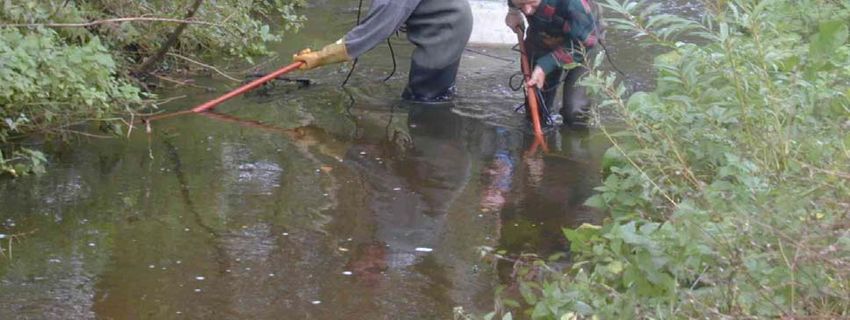
General introduction

This manual contains three parts. Part I introduces the Water Framework Directive and the
basic ideas of the Index of Biotic Integrity. The advantages of fishes as indicators for
assessing the ecological quality in running waters are described.
Part II gives an overview of the European FAME project and its achievements. The main
features of the European Fish Index (EFI) are described and the field sampling procedures
required to collect suitable data are briefly discussed. The limitations of the newly developed
index are also demonstrated. Additionally, the EFI software tool also enables sites to be
assigned to “European Fish Types” (EFT) defined within the FAME project. Descriptions of
the EFTs are given based on the species composition of the fish assemblages.
Part III is the instruction manual to the software, it details the different steps required to
obtain the EFT, the EFI and ecological status assessment for new sites.

                                               7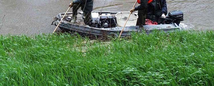
Part I: Introduction

1. The Water Framework Directive (WFD)

The aim of the WFD is to create a European framework for the protection of inland surface
waters, transitional waters, coastal waters and groundwater (EU Water Framework Directive,
2000). Its principal objective is to protect, enhance and restore all bodies of surface waters
with the aim of achieving a good status by 2015 (WFD Article 4). The WFD requires member
states to assess the ecological quality status (EcoQ) of their water bodies (Article 8). The
EcoQ is based on the status of biological quality elements supported by hydromorphological
and chemical/physicochemical quality elements. Consequently, the implementation of the
WFD requires appropriate and standardised methods to assess ecological status. The four
biological elements to be considered in rivers are (1) phytoplankton, (2) phytobenthos and
macrophytes, (3) benthic invertebrate fauna and (4) fish fauna.
The WFD prescribes the following steps for ecological status assessment (Figure 1 below):

 classify river         define reference
     types                 conditions
                                                         assess              assign quality
                                                        deviation                status
                       sample monitoring
                             sites                                              high (1)

                                                                                good (2)

                                                                            moderate (3)

                                                                                poor (4)

                                                                                 bad (5)

           Figure 1: Steps prescribed in the WFD for ecological status assessment

Initially, river types have to be defined. Each type is described by abiotic parameters (System
A or B, WFD Annex II 1.2) and verified by the biota. For each type, reference conditions with
no or only very minor anthropogenic alterations have to be defined for each biological quality
element. Reference conditions may be derived from actual data, historical data or modelling

                                              8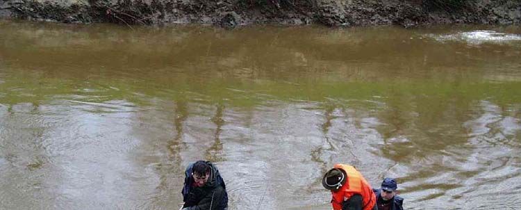
techniques. Finally, an assessment method for each quality element has to be developed. The
assessment of a specific site is based on its deviation from type-specific reference conditions.
The status of the fish fauna should be assessed with the following criteria: species
composition, abundance, sensitive species, age structure and reproduction (Annex V 1.2.1).
The WFD distinguishes between five levels of ecological status: (1) high status, (2) good
status, (3) moderate status, (4) poor status and (5) bad status. The approach adopted by the
FAME project was designed to follow the principles of the WFD summarised briefly here
(see Part II).

2. Fish-based ecological assessment methods in Europe

Currently, different fish-based methods are used in Europe, while most countries have not yet
included fish in their routine monitoring programs. Thus, the successful implementation of the
WFD depends on the provision of reliable and standardised assessment tools. This was the
motivation for the EC-funded FAME project. The project aimed to develop, evaluate and
implement a fish-based assessment method for the ecological status of European rivers to
guarantee coherent and standardised monitoring throughout Europe.

3. What is an Index of Biotic Integrity (IBI)?

The principle of the Index of Biotic Integrity (IBI, Karr 1981) is based on the fact that fish
communities respond to human alterations of aquatic ecosystems in a predictable and
quantifiable manner. An IBI is a tool to quantify human pressures by analysing alterations of
the structure of fish communities. The original IBI (Karr 1981) uses several components of
fish communities, e.g. taxonomic composition, trophic levels, abundance and fish health.
Each component is quantified by metrics (e.g. proportion of intolerant species). A metric is a
measurable variable or process that represents an aspect of the biological structure, function,
or other component of the fish community and changes in value along a gradient of human
influence. Depending on the underlying biological hypotheses, a metric may decrease (e.g.
number of sensitive species) or increase (e.g. number of tolerant species) with the intensity of
human disturbances.

                                               9
4. Why fish?
Fishes have proved their suitability as indicators for human disturbances for many reasons:
− Fishes are present in most surface waters.
− The identification of fishes is relatively easy and their taxonomy, ecological
requirements and life histories are generally better known than in other species groups.
− Fishes have evolved complex migration patterns making them sensitive to continuum
interruptions.
− The longevity of many fish species enables assessments to be sensitive to disturbance
over relatively long time scales.
− The natural history and sensitivity to disturbances are well documented for many
species and their responses to environmental stressors are often known.
− Fishes generally occupy high trophic levels, and thus integrate conditions of lower
trophic levels. In addition, different fish species represent distinct trophic levels:
omnivores, herbivores, insectivores, planktivores and piscivores.
− Fishes occupy a variety of habitats in rivers: benthic, pelagic, rheophilic, limnophilic,
etc., Species have specific habitat requirements and thus exhibit predictable responses
to human induced habitat alterations.
− Depressed growth and recruitment are easily assessed and reflect stress.
− Fishes are valuable economic resources and are of public concern. Using fishes as
indicators confers an easy and intuitive understanding of cause effect relationships to
stakeholders beyond the scientific community.
10Part II: The European research project FAME
1. Introduction
FAME stands for ‘Development, Evaluation and Implementation of a standardised Fish-based
Assessment Method for the Ecological Status of European Rivers’ and is a contribution to the
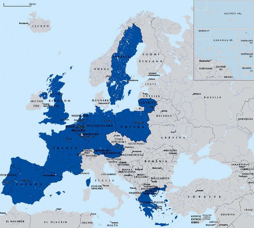
Water Framework Directive. The following 12 countries participated in the project: Austria,
Belgium, France, Germany, Greece, Lithuania, Poland, Portugal, Spain, Sweden, the
Netherlands and the United Kingdom.
Figure 2: Countries participating in FAME
FAME developed and tested several fish-based assessment methods for the ecological status
of rivers. Finally, the European Fish Index (EFI) was selected as the method most suitable to
11meet the requirements of the WFD. The FAME consortium comprised both scientific
(academic institutions) and applied (national institutions responsible for water management)
partners to ensure the successful uptake of the FAME tool by end-users and to support its
implementation into routine monitoring for the WFD.
2. Basic tools of FAME used to develop the EFI
FIDES (Fish Database of European Streams) is a large database of about 15 000 fish samples
covering 8 000 sites from 2 700 rivers in 16 European eco-regions contributed by 12 countries
(Figure 3). For each site information about the sampled fish, abiotic variables and human
pressures was collected. FIDES also includes a comprehensive list of European freshwater
fish species assigned to ecological guilds according to their ecological characteristics. This
information was used to calculate metrics for the newly developed index (Annexes 3 and 4).
Table
HISTORICAL
Site_code
Help table
ECOREGION
Site_code Table
SITE Ecoregion
Help table
Country_ COUNTRIES
abbreviation
Help table
Site_code, La, Lo, Table FISHING
Reporter_code REPORTER
Reporter_code, OCCASION
Date
Table
METRICS
Site_code, La, Lo, Table Species
Date, Species CATCH Help table
TAXA and
GUILDS
Site_code, La, Lo,
Date, Species
Table
Table
LENGTH
LENGTH
CLASS
Figure 3: Structure of the central database, FIDES (Fish Database of European Streams,)
and relations between tables (La, Lo = latitude and longitude)
123. The European Fish Index (EFI)
The European Fish Index (EFI) is based on a predictive model that derives reference
conditions for individual sites and quantifies the deviation between predicted and observed
conditions of the fish fauna. The ecological status is expressed as an index ranging from 1
(high ecological status) to 0 (bad ecological status).
1. In the first step the EFI uses data from single-pass electric fishing catches to calculate
the assessment metrics (Figure 4, p. 17). The EFI employs 10 metrics belonging to the
following ecological functional groups: trophic structure, reproduction guilds, physical
habitat, migratory behaviour and capacity to tolerate disturbance in general (Table 1,
Annex 4). Six metrics are based on species richness and four on densities.
Table 1: The 10 metrics used by the EFI and their response to human pressures
(↓ = decrease; ↑ = increase of metric)
Selected metrics Response to human pressures
Trophic level
1. Density of insectivorous species ↓
2. Density of omnivorous species ↑
Reproduction strategy
3. Density of phytophilic species ↑
4. Relative abundance of lithophilic species ↓
Physical habitat
5. Number of benthic species ↓
6. Number of rheophilic species ↓
General tolerance
7. Relative number of intolerant species ↓
8. Relative number of tolerant species ↑
Migratory behaviour
9. Number of species migrating over long distances ↓
10. Number of potamodromous species ↓
2. In the second step a theoretical reference value, indicating no or only slight human
disturbances (equals high or good status), is predicted for each metric using
environmental variables by means of a multilinear regression model calibrated with
FIDES reference data (p. 17, Figure 4, step 2). Ten environmental factors and three
sampling variables pertaining to the specific site and sampling strategy are used to
predict reference values. Additional information on location, site name, sampling date
is required (Table 2, p. 16). Nine environmental variables account for local natural
13variability in fish communities (e.g. altitude, slope). One environmental variable, river
region, is used to explain regional differences. To identify the main river regions 36
hydrological units were defined using two criteria: each large basin (over 25 000 km2)
was considered as a separate unit characterised by its native fauna list, whereas all
smaller basins flowing to the same sea coast were grouped (IHBS Sea area codes).
Finally, the 36 hydrological units were grouped into 11 main river regions based on
the similarity of their native fish fauna (see Annex 2, Table 1 and Figure 1).
3. The residuals of the multilinear regression models are used to quantify the level of
degradation. Residuals are calculated as observed metric values minus theoretical
(predicted) metric values (p. 17, Figure 4, step 3).
4. Residual metric values scatter around the theoretical value. Impacted sites exhibit a
greater deviation from the theoretical value and thus are less likely to belong to the
reference residual distribution than unimpacted or only slightly impacted sites (p. 17,
Figure 4, step 4).
5. The metrics in the EFI are based on different units (e.g. number of species, number of
individuals). To make metrics comparable they are standardised through subtraction
and division by the mean and the standard deviation of the residuals of the reference
sites, respectively (p. 17, Figure 4, step 5).
6. As some standardised residuals values tend to increase with disturbance (i.e. density of
omnivorous species), whereas others decrease (i.e. density of insectivorous species,
Table 1, p. 13), they are transformed into probabilities (p. 17, Figure 4, step 6). This
transformation presents two main advantages. Firstly, all metrics will vary between 0
and 1, whereas the standardised residuals have no finite values, and secondly, all
metrics will have the same response to disturbance, i.e. a decrease. This final metric
value describes the probability for a site to be a reference site, i.e. a site belonging to
the two best ecological integrity classes (1 and 2). A site that fits perfectly with the
prediction (theoretical value) will have a final metric value of 0.5, whereas the value
for an impaired site will decrease when disturbance intensity increases. If the final
probability value of the metric is higher than 0.5, the situation observed on the field is
better than the predicted one and the probability for these site to be an excellent site
(ecological integrity class 1) increases.
7. The final European Fish Index (EFI) is obtained by summing the ten metrics, and then
by rescaling the score from 0 to 1 (Figure 4, step 7).
148. The final step is to assign index scores to ecological status classes. Class boundaries
have been defined based on the comparison of data sets with different degrees of
human pressures. The class boundaries for the five status classes are shown in Figure
4, step 8 (p. 17).
The EFI was validated within the FAME project with independent data stets. The EFI was
also validated against a pre-classification of site status based on assessment of human
pressures to the hydrology, morphology and chemical quality of the water body. The EFI was
able to discriminate between non-impacted and impacted sites in about 80 % of the cases.
15Table 2: Abiotic variables and sampling method variables required for the EFI to predict
reference conditions (variable codes for the EFI software in italics)
Environmental variables describing the sampling site
Altitude* The altitude of the site in metres above sea level (data source: maps).
E_altitude
Are there natural lakes present upstream of the site? Answer Yes or No. Only
Lakes upstream applicable if the lake affects the fish fauna of the site, e.g. by altering thermal regime,
E_lakeupstream flow regime or providing seston. Use national definition of a lake (see glossary Annex
5).
Distance from source in kilometres to the sampling site measured along the river. In
Distance from source* the case of multiple sources, measurement shall be made to the most distant upstream
E_distsource source (data source: maps).
Permanent: never drying out.
Flow regime Summer dry: drying out during summer (data source: gauging station or hydrological
E_flowregime reports).
Wetted width in metres is normally calculated as the average of several transects
Wetted width* across the stream. The wetted width is measured during fish sampling (performed
E_wettedwidth manly in autumn during low flow conditions) (data source: field measurement).
Siliceous or calcareous (based on dominating category) (data source: geological
Geology E_geotypo maps).
Mean air temperature* Yearly average air temperature measured for at least 10 years. Given in degrees
E_tempmean Celsius (°C) (data source: nearby measuring site, interpolated data).
Slope of streambed along stream expressed as per mill, m/km (‰). The slope is the
Slope* drop of altitude divided by stream segment length. The stream segment should be as
E_slope close as possible to 1 km for small streams, 5 km for intermediate streams and 10 km
for large streams (Data source: maps with scale 1:50 000 or 1:100 000).
Size of catchment Size of the catchment (watershed) upstream of the sampling site.
E_catchclass Classes are:(1) Metric calculation (2) Metric prediction
“observed metrics” calibration data set for development of reference models
Multilinear regression model Multilinear regression model
Value of metric 1
Number of fish .
....
Metric 10
Metric 1
caught per .
species .
Value of metric 10
Environmental descriptors Environmental descriptors
(3) Residual calculation
(8) Assignment to Residual metric = observed metric – theoretical metric
predicted
ecological status class reference
values
....
metric 1
Status class Score
residuals
High: [0.669 – 1.000] deviation
EFI Good: [0.449 – 0.669[
from
reference
European Moderate: [0.279 – 0.449[ Environmental descriptors (e.g. altitude, slope)
Fish Poor: [0.187 – 0.279[
Index
Bad: [0.000 – 0.187[
(4) Residual distribution
(7) Index calculation metric range
Index rescaling from 0 to 1 observed theoretical metric value
Frequency
metric
values
residual distribution
....
of calibration data
10
Index = ∑ metricsx - 50 % -25 % 0 25 % 50 %
x=1 Residual metric
(example: percentage of intolerant species)
(6) Transformation to probabilities (5) Residual standardisation
metric range
1.0
0.75
Probability
observed theoretical metric value
Frequency
metric
values
....
0.50
probability to
theoretical
metric
....
be a reference 0.25 observed value
site metric
values
-4 -2 0 2 4
0
-4 -2 0 2 4 Standardised residual metric
Standardised residual metric
Figure 4: The methodology of the EFI: In step 3 to 6 two examples, a reference site (green)
and a disturbed site (red) are shown
17Example of application
To calculate the EFI the information about the environmental variables and the fish caught at
a given site are needed (see example in Table 3). Based on the number of fish caught, the
software calculates first the value of the metrics (Figure 5, p. 19). These are called the
observed metric values. In a second step, the model predicts, as a function of the
environmental variables, the theoretical metric values. These are the reference values
expected at a particular site. Finally, the model quantifies the deviation from the theoretical
reference condition by calculating for each metric the difference between the observed and
theoretical value. This is called the residual metric value. The residual metric value is
standardised into a probability metric, indicating the probability of a site being unimpacted,
with values ranging from 0 (bad status) to 1 (high status). The rescored sum of these ten
values gives the final EFI (see also part III).
Table 3: Example of site information and environmental variables - River Dropt, France
Variables describing the location, name of site and date of fishing
Site code FR05470095
Latitude 44.3816N
Longitude 00.4411E
Date 09/10/1985
River region Garonne
River name Dropt
Site name Villereal
Environmental variables
Geology Calcareous
Size of catchmentAssigning species to guilds
Number of fish caught Intol Tol Benth Rheo Litho Phyto Insec Omni Diadr Pota
Gobio gobio 225 0 0 1 1 0 0 0 0 0 0
Alburnus alburnus 69 0 1 0 0 0 0 0 1 0 0
Rutilus rutilus 41 0 1 0 0 0 0 0 1 0 0
Chondrostoma toxostoma 30 1 0 1 1 1 0 0 1 0 1
Phoxinus phoxinus 22 0 0 0 1 1 0 0 0 0 0
Leuciscus cephalus 20 0 0 0 1 1 0 0 1 0 1
Barbatula barbatula 15 0 0 1 1 1 0 0 0 0 0
Lepomis gibbosus 11
0 1 0 0 0 0 1 0 0 0
Rhodeus sericeus 9
1 0 0 0 0 0 0 0 0 0
Barbus barbus 2
0 0 1 1 1 0 0 0 0 1
Leuciscus leuciscus 2
0 0 0 1 1 0 0 1 0 0
Perca fluviatilis 2
Anguilla anguilla 0 1 0 0 0 0 0 0 0 0
1
0 1 1 0 0 0 0 0 1 0
Calculating “observed metrics”
Insectivorous species (Insec) 275 ind.ha-1
Omnivorous species (Omni) 4050 ind.ha-1
Phytophilous species (Phyto) 0 ind.ha-1
Lithophilic species (Litho) 19 % ind.
Benthic species (Benth) 5 species
Rheophilic species (Rheo) 7 species
Diadromous species (Diadr) 1 species
Potamodromous species (Pota) 3 species
Intolerant species (Intol) 15 % species
Tolerant species (Tol) 38 % species
Figure 5: Process of converting species data into observed metric values - River Dropt,
France
The environmental data, fishing method and number of fish caught obtained during the survey
in the river Dropt (France) are given as an example (Table 3, p. 18). Figure 5 (p. 19)
illustrates how the species abundance data are converted into observed metric values. Table 4
(p. 20) shows the observed, theoretical and probability metric values for the French example.
To obtain the final EFI for the site the ten probability metric values are summed (example
River Dropt: total = 5.334; see Table 4, p. 20) and rescaled from zero to one (example River
Dropt: EFI = 0.5334).
Each site is assigned to an ecological status class according to the EFI score obtained. The
final ratings of the index for the five integrity classes are shown in Figure 4, step 8 (p. 17).
19The site from the River Dropt with an EFI of 0.53 is assigned to class 2 (good ecological
status).
Table 4: Observed, theoretical and probability metric values - River Dropt, France
Metrics Observed values Theoretical values Probability metric
values
Insectivorous species 275 ind.ha-1 383 ind.ha-1 0.423
Omnivorous species 4050 ind.ha-1 255 ind.ha-1 0.099
Phytophilic species 0 ind.ha-1 5 ind.ha-1 0.912
Lithophilic species 19 % ind 57 % ind 0.032
Benthic species 5 species 4.1 species 0.658
Rheophilic species 7 species 5.9 species 0.677
Diadromous species 1 species 0.5 species 0.841
Potamodromous species 3 species 1.5 species 0.894
Intolerant species 15 % species 17 % species 0.379
Tolerant species 38 % species 37 % species 0.419
Total 5.334
4. Limitations of the EFI
This index has been developed for sites located in the ecoregions presented in Annex 2. A
sufficient number of sites was available in 11 of the 25 European ecoregions. Therefore, the
EFI should not be applied in areas with a fish fauna deviating from those of the tested
ecoregions. The EFI should not be used (or only used with caution) in e.g. Mediterranean
rivers with high proportion of endemic species or in the rivers of the south-eastern part of
Europe which support fish communities that differ greatly in species composition. Although
the validation of the EFI also proved its applicability for large rivers the index should be used
with caution in the lowland reaches of very large rivers such as the Rhine and Danube as no
reference sites from these reaches have been used for the calibration of the EFI. In those cases
the EFI uses only extrapolated predictions based on the trends observed in the models.
The statistical models that are used for the EFI reflect the average response of fish
communities to environmental conditions. The application of the EFI for particular
environmental situations such as the outlet of lakes or predominantly spring fed lowland
rivers might cause problems. However, those unique situations are mostly spatially limited
and are therefore less important in countrywide monitoring programmes.
20Only fish data obtained with single-pass electric fishing may be used to calculate the EFI. If
data from multiple passes are used (i.e. same site fished several times and catches cumulated)
the EFI produces erroneous results.
As the EFI is a statistical method to assess the community composition, a minimum number
of data is required to run the software. For a given site, 30 specimens is the minimum sample
size required to be able to calculate the EFI with appropriate statistical confidence. When
fewer specimens were caught the software still allows you to calculate the EFI, but the results
must be considered with care. The same applies when the sampled area is smaller than 100
m². Consequently, when no fish occur at a site, this method is not applicable. Two cases could
be problematic and the EFI should be used with care: (1) undisturbed rivers with naturally low
fish density and (2) heavily disturbed sites where fish are nearly extinct. In the first case, fish
are close to the natural limits of occurrence and therefore might not be good indicators for
human impacts. The occurrence of fish in those rivers is highly coincidental and therefore not
predictable. If the very low density is caused by severe human impacts more simple methods
or even expert judgement are sufficient to assess the ecological status of the river.
The EFI provides a continuous score from 0 to 1. The discrimination between ecological
classes, i.e. between unimpacted and impacted sites was based on validated statistical tests.
However, due to the low number of minimally disturbed sites (class 1) and heavily disturbed
sites (class 5) in FIDES, the limits between class 1 and 2 and class 4 and 5 were set arbitrarily.
Therefore, the probability to misclassify sites of high and bad status is higher than for sites of
good, moderate and poor status.
The model was developed using data from sites with environmental characteristics ranging
between specific limits. These values are given in Table 5. Your site should have
characteristics within these ranges in order to obtain a confident EFI.
Table 5: Minimum, median and maximal values of environmental characteristics
Characteristics Minimum Median Maximum
Distance from source [km] 0.0 20.0 990.0
Altitude [m.a.s] 0.0 56.0 1950.0
Slope gradient [m.km-1] 0.50 7.00 199.00
Wetted width [m] 0.5 7.0 1600
Mean air temperature [°C] -2.0 10.0 16.0
The WFD requires the use of species composition, abundance, sensitive species, age structure
and reproduction within assessment criteria. The ten metrics used in the EFI only represent the
21species composition, abundance and sensitive species criteria. However, at the time the FAME
project was developed, the data on fish length necessary to calculate metrics for age structure
and reproduction were not available in all European countries. These metrics could be
integrated in a future version of the EFI.
225. European Fish Types (EFT)
The European Fish Index predicts reference conditions specifically for each site - thus it is not
based on pre-classified river types. To be in accordance with the WFD European Fish Types
were defined as accompanying tool. Based on FIDES references sites spread over 11
ecoregions, 15 European Fish Types were identified.
Table 6: The 15 European Fish Types and relative species composition (%), only species
>2% are listed (species >12 % in bold)
European Fish Type
1 2 3 4 5 6 7 8 9 10 11 12 13 14 15
Number of Sites 148 365 553 229 1130 832 69 84 7 81 9 446 148 67 432
Fish species
Salmo trutta fario 94 81 43 37 11 5 45 7 25 14 9 4 1 3
Cottus gobio 0 14 38 5 19 12 4 13 17 0 1 0
Phoxinus phoxinus 0 1 7 17 21 31 9 7 15 3 2
Barbatula barbatula 0 3 13 14 13 1 1 1 1 3
Anguilla anguilla 3 0 0 0 16 1 0 3 0 9 1
Leuciscus souffia 0 12 0
Thymallus thymallus 1 1 0 0 1 45 11 18 1 0 0
Salmo salar 2 1 0 7 0 45 9 3 0
Cottus poecilopus 2 0 1 5 47 0 4
Leuciscus carolitertii 0 36
Chondrostoma polylepis 1 23
Rutilus arcasii 0 14
Barbus bocagei 10
Salmo trutta lacustris 0 0 0 100 6 2
Salmo trutta trutta 0 0 0 0 1 40 0
Barbus meridionalis 0 1 0 53
Leuciscus cephalus 0 1 4 2 5 1 2 0 11 10 8
Barbus haasi 8
Gasterosteus aculeatus 0 2 1 1 1 0 39 1
Alburnoides bipunctatus 0 0 0 3 0 15 1
Rutilus rutilus 0 0 0 3 6 1 2 10 37
Alburnus alburnus 0 0 4 0 0 6 7
Gobio gobio 0 0 1 6 1 5 0 0 1 4 7
Perca fluviatilis 0 0 0 0 3 1 4 1 6
Lota lota 0 0 0 0 0 1 4 0 2
Leuciscus leuciscus 0 0 1 4 1 2 4
Esox lucius 0 0 0 1 1 1 1 3
Barbus barbus 0 0 1 0 1 1 0 0 2
Nine abiotic variables were selected to discriminate between the 15 European Fish Types
(Table 7, p. 24). These variables are used to classify the river type of a new site that has to be
assessed.
23The limitations defined for the EFI in chapter 4 are principally also valid for the EFT. The
calculation of the EFT should only be done within the spatial and environmental limits the
method was designed for.
Table 7: Distribution of European fish types across ecoregions and abiotic variables (mean
values) discriminating between the 15 European Fish Types
Distance from source (km)
Mean air temperature (°C)
Wetted width (m)
Slope (m/km)
X co-ordinate
Y co-ordinate
Altitude (m)
EFT
1 856 7 8.1 18.9 15 n.a. n.a.
2 633 9 6.1 22.1 14 n.a. n.a.
3 173 6 9 9.5 12 n.a. n.a.
4 487 7 9.5 16.9 16 n.a. n.a.
5 41 9 10 3.5 30 n.a. n.a.
6 110 12 9.6 2 48 n.a. n.a.
7 562 33 7.1 3.2 110 n.a. n.a.
8 61 54 7.4 2.8 90 n.a. n.a.
9 582 19 -0.1 35.4 26 n.a. n.a.
10 214 21 13.8 7 43 n.a. n.a.
11 718 9 0.7 19.5 6 n.a. n.a.
12 45 46 8.1 3.9 65 n.a. n.a.
13 291 5 13.4 23.3 14 n.a. n.a.
14 61 30 6.1 0.7 151 n.a. n.a.
15 120 163 9.8 0.9 273 n.a. n.a.
246. Collecting data for the EFI
To employ the assessment method and to define the European Fish Type the following
procedure should be applied. The different steps are explained in the text below.
Site selection (page 26)
Collecting data about (Table 2, p. 16) Fish sampling (page 26-29)
1. location
2. environment
3. sampling procedure
Collecting fish data (Annex 1)
Input of data into database (e.g. FIDES or EFI)
Assessment of site with the EFI software
Import7:ofDifferent
1.Figure steps to apply
data to software the assessment method
(page)
2. Run the software
3. Output
• Identification of European Fish Type (EFT)
• Calculation of observed, theoretical and probability metrics
• Calculation of EFI score and assignment to status class
Figure 6: Different steps required to apply the assessment method
25Site selection
The selected site should be representative, within the river segment, in terms of habitat types
and diversity, landscape use and intensity of human pressures.
A river segment is defined as:
1 km for small rivers (catchment1000 km²)
A segment for a small river will thus be 500 m upstream and 500 m downstream of the
sampling site.
Environmental variables and sampling methods
To model the reference situation for the sampled site the variables from Table 2 (p. 16) should
be recorded in the data sheet (see field protocol in Annex 1-Table 2 and environmental and
method data in part III).
Fish sampling
To calculate the index only fish data obtained by electric fishing can be used. Standardised
electric fishing procedures are precisely described in the CEN directive, “Water Analysis –
Fishing with Electricity (EN 14011; CEN, 2003) for wadable and non-wadable rivers.
Fishing procedures and equipment differ depending upon the water depth and wetted width of
the sampling site. The selection of waveform, DC (Direct Current) or PDC (Pulsed Direct
Current), depends on the conductivity of the water, the dimensions of the water body and the
fish species to be expected. AC (Alternating Current) is harmful for the fish and should not be
used. The fishing procedure is summarised below, separately for wadable and non-wadable
rivers. In both cases, fishing equipment must be suitable to sample small individuals (young-
of-the-year).
In the Tables 9 and 10 (p. 28 and 29), the river width corresponds with wetted width.
According to the CEN-standard, the main purpose of the standardised sampling procedure is
to record information concerning fish composition and abundance; therefore, no sampling
period is defined (according to CEN). However, FAME agreed on a sampling period of late
26summer/early autumn except for non-permanent Mediterranean rivers where spring samples
may be more appropriate.
Concerning the minimum river length to be sampled, because of the variability of habitats and
fish communities within rivers sections and in order to ensure accurate characterisation of a
fish community, electric fishing at a given site must be conducted over a river length of 10 to
20 times the river width, with a minimum length of 100 m. However, in large and shallow
rivers (width >15 m and water depth 0.7 m) and variety of habitats makes prospecting the entire area
impossible. Therefore, a partial sampling procedure is applied covering all types of habitats to
obtain a representative sample of the site. Qualitative and semi-quantitative information can
be obtained by using conventional electric fishing with hand held electrodes in the river
margins and delimited areas of habitat. Alternatively, where resources exist capture efficiency
can be improved by increasing the size of the effective electric field relative to the area being
fished by increasing the number of catching electrodes (electric fishing boats with booms).
Arrays comprising many pendant electrodes can be mounted on booms attached to the bows
of the fishing boat. The principal array should be entirely anodic with separate provision
being made for cathodes. Depending upon water conductivity, the current demands of
multiple electrodes can be high and large generators and powerful control boxes may be
needed (Table 9, p. 29).
27Table 8: Rivers < 0.7 m depth = wadable rivers
Waveform selection: DC or PDC
Number of anodes: One anode per 5 m width
Number of hand-netters: Each anode followed by 1 or 2 hand-netters (mesh
size of 6 mm maximum) and 1 suitable vessel for
holding fish.
Number of runs: One run
Time of the day: Daylight hours
Fishing length: 10 - 20 times the wetted width, with a minimum
length of 100 m
Fished area: river width 15 m: Several separated sampling
areas are selected and prospected within a
sampling site, with a minimum of 1000 m² (partial
sampling method)
Fishing direction: Upstream
Movement: Slowly, covering the habitat with a sweeping
movement of the anodes and attempt to draw fish
out of hiding.
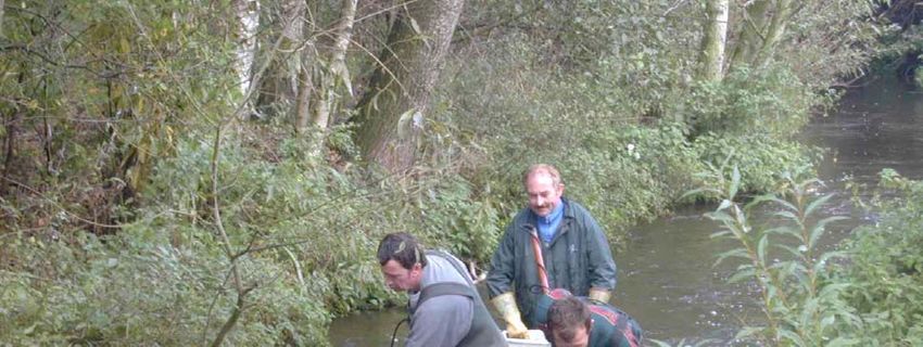
Stop nets: Used if necessary and feasible
Picture 1: Electric fishing in a wadable river
28Table 9: Rivers > 0.7 m depth = non-wadable rivers (boat fishing)
Waveform selection: DC or PDC
Number of anodes: Depending on boat configuration
Number of runs: One run
Time of the day: Daylight hours
Fishing length: 10 -20 times the wetted width, with a minimum length of 100 m
Fished area: Both banks of the river or a number of sub-samples proportional to
the diversity of the habitats present with a minimum of 1000 m²
(partial sampling method)
Fishing direction: Normal flow: downstream in such a manner as to facilitate good
coverage of the habitat, especially where weed beds are present or
hiding places of any kind are likely to conceal fish
High flow: upstream
Low flow: not necessary to match boat movement to water flow, and
the boat can be controlled by ropes from the bank side if required
Movement: Slowly, covering the habitat with a sweeping movement of the
anodes or drifting with the boom along selected habitats and
attempting to draw fish out of hiding.
Stop net Used if necessary and feasible
Picture 2: Electric fishing from a boat
29Fish data
To calculate the EFI, each collected specimen should be identified to species level by external
morphological characters and the total number of specimens per species should be recorded
on the field protocol data sheet (see Annex 1-Table 1: fish data).
The EFI software or the FAME database FIDES can be used for data input. The blank FIDES
database structure can by downloaded from the FAME homepage http://fame.boku.ac.at.
30Part III: A manual for application
First copy the software EuropeanFishIndex.xls to a directory of your choice. In addition the
program file Comdlg32.ocx needs to be installed in C:\WINDOWS\SYSTEM\ if not already
present there. You must not rename the file EuropeanFishIndex.xls as this would cause
problems in running the software. The software was developed for Microsoft Office version
2000 and 2003. Running the software with older Microsoft Office versions is not
recommended as some features may not function properly.
1. Preparing data in MS Excel: data organisation and format
Before using the software you have to prepare your data in separate Microsoft Excel® file.
Use two different files, one for the EFI and one for the EFT. In this manual these files are
referred to as the EFI-file and EFT-file.
You must make sure that your Excel is not set to the R1C1 reference style. The software
requires that columns are referenced by letters, numbers indicate rows. If this is not so you
change this by selecting in the opened Excel file (e.g. spreadsheet 1) the “Tools” in the menu
(1), then select “Options” (2).
Spreadsheet 1
1
2
31Choose “General” (step 1 in spreadsheet 2) and make sure that in “settings” the ‘R1C1
reference style’ option (step 2) is not highlighted.
Spreadsheet 2
1
2
Both files should contain variables formatted in an appropriate way so that the software can
recognise the variable names, the variable values and variable types. The column sequence is
not important.
In the EFI-file you need to include a list of 19 obligatory variables. Additional variables can
be included but will not be used to calculate the European Fish Index (EFI.).
Table 2 (Part II, p. 16) gives the exact spelling of the 19 obligatory variables to be included
(variable codes in 1st column are in italics). Variable names are case-sensitive! If you make a
mistake in the variable name (incorrect spelling) or use an unexpected value, the software will
propose a list of solutions in a pop-up menu (see example in data control). Make sure that you
use the right units (metres for altitude, kilometres for distance from source, metres for
wetted width, degree Celsius for mean air temperature, per mill (m/km, ‰) for slope and m2
for fished area). Variable names and data should be checked carefully to avoid time
consuming corrections once you use the software. Make sure you have no empty cells for the
32obligatory variables. Another way to prepare the EFI-file is to download the EFI-input-file
from the FAME web site (http://fame.boku.ac.at) and use the template to store your own data.
The river regions (variable E_riverregion) aggregated to river groups are represented in
Annex 2. Use the correct spelling of the river region names as indicated in Annex 2-Table 1.
In addition you can include in the data file extra information about the ecoregion. The
ecoregion is defined according to the Illies’ classification and the WFD (Annex 2-Table 2,
Figure Annex_2-1).
You can include extra data. However, they will not be taken into account for the EFI
calculation. If you add extra variables do not use the prefix ‘E_’.
In the same EFI-file you add in the next columns the fish data, i.e. number of specimen, with
each species in a separate column. Annex 3 gives the names of the fish species used in the
EFI. The species variables must have the prefix ‘S_’ before the species name
(S_Genus_species). This naming procedure must be respected whether the species name is
listed or not. If you add a new species do not forget this prefix. The new species, however,
will not be taken into account for the EFI calculation. A mistake can be corrected using a list
that the software proposes in a pop-up menu (see example).
You have now completed your data preparation. These data can now be used to calculate the
EFI. Spreadsheet 3 gives a detailed example of what your prepared Excel spreadsheet should
look like.
33Spreadsheet 3
Extra variable: no Environmental variables Species names prefix
E_prefix prefix E_ S_
In the EFT-file you must include 9 obligatory variables. Table 2 (Part II, p. 16) gives the
exact spelling of the 9 variables to be included. Variable names are case-sensitive! If you
make a mistake in the variable name (incorrect spelling), the software will propose a list of
solutions in a pop-up menu (see example in data control).
The variable names (Table 2, p. 16) and data should be checked carefully to avoid time
consuming corrections once you use the software. Make sure you have no empty cells for the
obligatory variables as the software does not check for empty cells in the EFT procedure. If
empty cells are in your data the calculated EFT will be wrong! In addition, for the EFT
calculation the software does not check for unexpected values. Again additional variables can
be included but will not be used to calculate the European Fish Type (EFT). If you add extra
data do not use the prefix ‘E_’. Once you have completed your data preparation, they can be
used to calculate the EFT.
342. Installing the software
Start by opening an empty Excel file and activate the Visual Basic Application (VBA). You
can do that by typing simultaneously the keys “Alt” + “F11” or via the menu by activating
“Tools” (1), “Macro” (2), Select “Visual Basic Editor” (3)
Spreadsheet 4
1
2
3
35Once you have activated the VBA the following dialog box appears.
Microsoft Visual Basic dialog 1
1
Select “Tools” in the menu (1). In the next dialog screen select “References” (2).
Microsoft Visual Basic dialog 2
2
36In the new dialog box (Microsoft Visual Basic dialog 3), you need to activate “Microsoft
Common Dialog Control 6.0”. If you cannot find it you’ll have to import it as follows: use the
browser and go to Windows/System/comdlg32.ocx. This is the required file and you activate
it after selecting. “Microsoft Common Dialog Control 6.0” will appear in the dialog box. Then
click “OK” (1).
Microsoft Visual Basic dialog 3
1
Once this is done successfully return to the Excel file you have previously opened. Select
“File”, next “Open” and select the “EuropeanFishIndex.xls” file. In the Excel spreadsheet a
message will appear that this file contains Macros. Click on “Enable Macros” (1) (spreadsheet
5).
37Spreadsheet 5
1
Now the file will be loaded and a new menu “Fame” will be created. However, if you have
problems loading the “EuropeanFishIndex.xls” file you will have to adjust the Excel security
level setting. In the Excel file select “Tools” (1) then “Macro” (2) and “Security” (3).
Spreadsheet 6
1
2
3
38Set Security to “Medium” or “Low” (1 in spreadsheet 7) and click “OK”.
Spreadsheet 7
1
Now, reload the “EuropeanFishIndex.xls” file and select the option to activate the Macros
(Spreadsheet 5). Click “OK” and spreadsheet 8 appears.
Spreadsheet 8
39Click “OK” and once it is loaded you will see in the menu bar that “Fame” has been added (1
in spreadsheet 9).
Spreadsheet 9
1
Note, that three worksheets are formed: result, metrics and history.
403. Entering new data in the software
You can now load your data into the software.
This section describes how to calculate the European Fish Index (EFI).
Click on the “Fame” menu (1 in spreadsheet 10). Choose “EFI method” (2) and select
“InputData” (3).
Spreadsheet 10
1
2 3
A common dialog box will be displayed to remind you that the slope should be expressed in
metres per km. Choose “Yes” if this is the case (spreadsheet 11). If you have not entered the
slope data as metres per km you will need to re-calculate these values in the EFI-file before
loading the data into the software and proceeding with the EFI calculation.
41Spreadsheet 11
Once you have confirmed the units of the slope variable, a message appears informing you
that you can start the program (spreadsheet 12). Click “OK”.
Spreadsheet 12
A common dialog box will be displayed to initiate the data import process (spreadsheet 13)
42Spreadsheet 13
Click “Start” to Click “Cancel”
begin the data to interrupt the
import data import
If you choose “Start” the standard MS Windows “Open” pop-up window will appear.
Spreadsheet 14
1
Now you select the file you have prepared to import. Accepted file formats are Excel files and
Text Files. In this example the ‘Input data’ file is imported (1 in spreadsheet 14). Once you
have selected the file, the file path is displayed. You can check if this is the required file
(spreadsheet 15).
43Spreadsheet 15
Click “OK” to confirm your choice and the file will be opened (spreadsheet 16).
Spreadsheet 16
1
When the file opens, the number of cells, rows and columns in the dataset is displayed (1).
The selected dataset is displayed in blue. Click “OK” to initiate the data verification process.
444. Data quality control with an example
The software will first check the species names in the imported file. Spreadsheet 17 shows the
example of a species e.g. “Salmo_trutta” which is not a valid variable name as it is not
present in the taxa list in that format.
Spreadsheet 17
Click “OK” to check
After clicking “OK” a pop-up help list with recognised fish species names will appear
(spreadsheet 18). A message informs you that you can now check the species name.
45Spreadsheet 18
You click “OK” and a pop-up asks you if the species is indeed a new species (spreadsheet
19).
Spreadsheet 19
Click “Yes” if it is Click “No” if it is a
a new species spelling mistake
If you click “Yes”, a message informs you that the species richness will be computed with the
new species. However, it will not be considered during the EFI calculation (spreadsheet 20).
46Spreadsheet 20
If you click “No” in spreadsheet 19, a message will appear telling you that you can now
correct the name (spreadsheet 21).
Spreadsheet 21
Click “OK” and a pop-up help list with valid fish species names (“Species selection” in
spreadsheet 22) appears.
47In this example Salmo_trutta_trutta is selected (1) and confirmed (2).
Spreadsheet 22
1
2
A pop-up will indicate if there are more mistakes in the species names or not. Following
verification of the species names a message will appear (spreadsheet 23) indicating that all
species names are correct and that the environmental variables will now be checked.
Spreadsheet 23
48Click “OK” and the software will now start to verify the environmental variable names. The
following spreadsheets illustrate two types of spelling mistakes. Spreadsheet 24 indicates that
the name ‘altitude’ was formatted incorrectly as ‘Altitude’. The variable names are case
sensitive!
Spreadsheet 24
Click “OK” and select the correct name. In this case ‘altitude’ (1) and confirm (2) (see
spreadsheet 25).
49Spreadsheet 25
1
2
In this example another mistake is present. The variable name ‘geotypol’ is misspelled
(spreadsheet 26).
Spreadsheet 26
Click “OK”, select the correct spelling (1 spreadsheet 27) and confirm the variable name (2).
50Spreadsheet 27
1
2
Once all names are checked and corrected and no more mistakes occur, a message appears:
“Names of Environmental Variables are correct, now checking values”.
Spreadsheet 28
Click “OK” to start the verification of the environmental variables values. In this example one
value has been entered incorrectly (spreadsheet 29). It is a value for the catchment class being
51indicated as ‘>10’. In this case it was miss-typed and it should be ‘
The software macro will continue, step by step, to check all values of the obligatory variables
required for the EFI (Table 2, p.16). Finally a message appears to confirm that the value
verification is completed (spreadsheet 31).
Spreadsheet 31

Click “OK” and the software will now check the number of fish caught and the value of the
fished area to verify if they comply with the EFI requirements. For each record that does not
meet the requirements the site code will be listed and a message displayed. Spreadsheet 32
shows a site where the surface area sampled is insufficient (less than 100 m²). You can choose
to keep (1) or delete (2) this record. If you choose to keep the record bear in mind that the
result should be treated with caution since the EFI is designed to work with results obtained
from sampling areas of at least 100 m².

                                              53
Spreadsheet 32
1 2
If no fish were caught in a certain sample a message appears informing you that the index
cannot be calculated and that this entry will be deleted (spreadsheet 33). Click “OK” to delete
such a record.
Spreadsheet 33
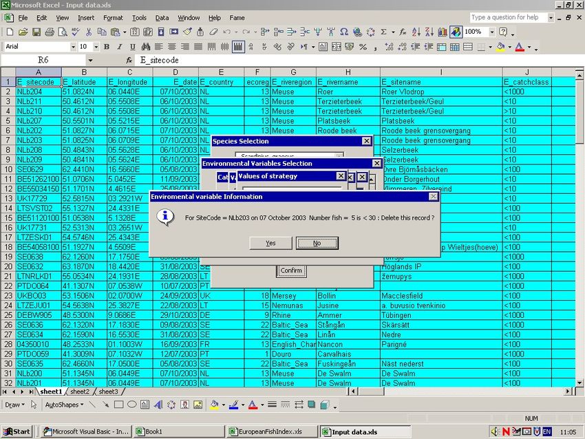
The EFI requires a minimum number of 30 specimens in a sample to make a proper
assessment of the site. When fewer fish are caught the result is not reliable. In this example
54(spreadsheet 34) there is a sample with a number of fish of more than 0 but less than the
required number (=30). This record can be kept (1) or deleted (2).
Spreadsheet 34
1 2
Once this control is finished the software lists the ‘Addresses of empty cells’. This informs
you of the number and location of missing values (empty cells). Click “OK”.
Spreadsheet 35
The next spreadsheet informs you on the number of samples deleted.
55Spreadsheet 36
Click “OK” and the imported file will appear.
Spreadsheet 37
Empty cells are highlighted in red. All validations are done and the software can now start to
compute the EFI.
565. Index calculation
In the “Fame” menu you select “EFI Method” (1), “Metrics calculation” (2).
Spreadsheet 38
1
2
The next message indicates that the EFI calculation can take a moment (spreadsheet 39). You
click “OK”.
57Spreadsheet 39
The software now starts to calculate the index. This calculation is done in two steps.
Step 1
Calculation of the observed metric values.
Spreadsheet 40
58The results of this calculation are automatically written in the worksheet “result”. There are
33 columns. The first column (column A) gives the calculated river group for each sample
(automatically defined based on the variable river region). In the second column (B) the total
number of species found in each sample is documented. In the third column (C) the total
number of individuals per hectare (first run) is calculated. From the 4th to the 13th column (D-
M) the calculated metric values are represented (abbreviations see Table 10). The
Environmental variables, as given in the input-file, are copied to the 14th to 33rd columns (N-
AG).
Table 10: Metrics and abbreviations in result spreadsheet, ‘MA’ metric abbreviations used in
metrics spreadsheet. N.ha = number per hectare; n.sp = number of species; perc.nha =
percent of number per hectare; perc.sp = percent number of species
Metric abbreviation Metric MA
n.ha.Fe.insev Density of insectivorous species INSE
n.ha.Fe.omni Density of omnivorous species OMNI
n.ha.Re.phyt Density of phytophilous species PHYT
perc.nha.Re.lith Relative abundance of lithophilous species LITH
n.sp.Hab.b Number of benthic species BENT
n.sp.Hab.rh Number of rheophilic species RHEO
perc.sp.Intol Relative number of intolerant species INTO
perc.sp.Tol Relative number of tolerant species TOLE
n.sp.Mi.long Number of long migratory species LONG
n.sp.Mi.potad Number of potamodromous species POTA
The total number (N.sp.all) and density of species (Density.sp.all) values, shown in the result
worksheet, are metrics that are not used for the EFI computation.
59You can also read