Discovering Social Circles in Ego Networks
←
→
Page content transcription
If your browser does not render page correctly, please read the page content below
Discovering Social Circles in Ego Networks
JULIAN MCAULEY and JURE LESKOVEC, Computer Science Department, Stanford University

People’s personal social networks are big and cluttered, and currently there is no good way to automatically
organize them. Social networking sites allow users to manually categorize their friends into social circles
(e.g., “circles” on Google+, and “lists” on Facebook and Twitter). However, circles are laborious to construct
and must be manually updated whenever a user’s network grows. In this article, we study the novel task
of automatically identifying users’ social circles. We pose this task as a multimembership node clustering
problem on a user’s ego network, a network of connections between her friends. We develop a model for
detecting circles that combines network structure as well as user profile information. For each circle, we
learn its members and the circle-specific user profile similarity metric. Modeling node membership to multiple
circles allows us to detect overlapping as well as hierarchically nested circles. Experiments show that our
model accurately identifies circles on a diverse set of data from Facebook, Google+, and Twitter, for all of
which we obtain hand-labeled ground truth.
Categories and Subject Descriptors: H.3.3 [Information Search and Retrieval]: Clustering                                  4
General Terms: Algorithms, Experimentation
Additional Key Words and Phrases: Community detection, social circles, ego networks, machine learning
ACM Reference Format:
Julian McAuley and Jure Leskovec. 2014. Discovering social circles in ego networks. ACM Trans. Knowl.
Discov. Data 8, 1, Article 4 (February 2014), 28 pages.
DOI: http://dx.doi.org/10.1145/2556612

1. INTRODUCTION
Online social networks allow us to follow streams of posts generated by hundreds of
our friends and acquaintances. The people we follow generate overwhelming volumes
of information, and to cope with the ‘information overload,’ we need to organize our
personal social networks [Agarwal et al. 2008; Chen and Karger 2006; El-Arini et al.
2009]. One of the main mechanisms for users of social networking sites to organize
their networks and the content generated by them is to categorize their friends into
social circles. Social circles are lists of people that can be used for content filtering, for
privacy, and for sharing groups of users that others may wish to follow. Practically all
major social networks provide such functionality—for example, “circles” on Google+,
and “lists” on Facebook and Twitter.
  Examples of circles from a user’s personal social network are shown in Figure 1.
The “owner” of such a network (the “ego”) may form circles based on common bonds
and attributes between themselves and the users whom they follow. In this example,
the ego may wish to share their latest TKDD article only with their friends from
the computer science department, whereas their baby photos should be shared only
with their immediate family; similarly, they may wish to limit the amount of content

Author’s address: J. McAuley and J. Leskovec, Department of Computer Science, Stanford University,
Stanford, CA; email: {jmcauley, jure}@cs.stanford.edu.
Permission to make digital or hard copies of part or all of this work for personal or classroom use is granted
without fee provided that copies are not made or distributed for profit or commercial advantage and that
copies show this notice on the first page or initial screen of a display along with the full citation. Copyrights for
components of this work owned by others than ACM must be honored. Abstracting with credit is permitted.
To copy otherwise, to republish, to post on servers, to redistribute to lists, or to use any component of this
work in other works requires prior specific permission and/or a fee. Permissions may be requested from
Publications Dept., ACM, Inc., 2 Penn Plaza, Suite 701, New York, NY 10121-0701 USA, fax +1 (212)
869-0481, or permissions@acm.org.
c 2014 ACM 1556-4681/2014/02-ART4 $15.00
DOI: http://dx.doi.org/10.1145/2556612

          ACM Transactions on Knowledge Discovery from Data, Vol. 8, No. 1, Article 4, Publication date: February 2014.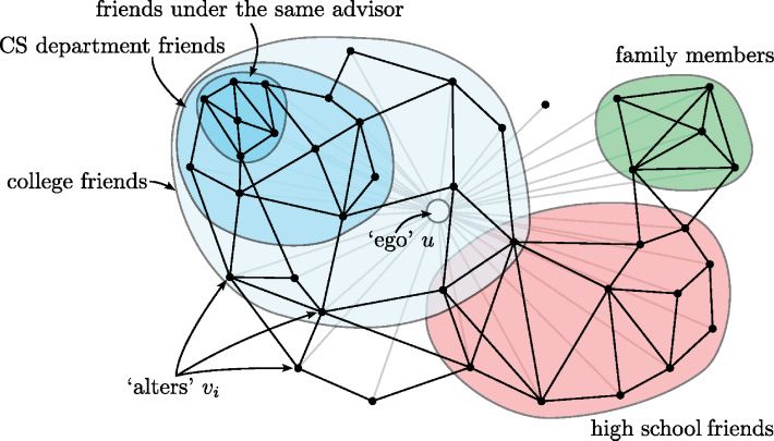
4:2                                                                                 J. McAuley and J. Leskovec

Fig. 1. An ego network with labeled circles. The central user, the ego, is friends with all other users (the
alters) in the network. Alters may belong to any number of circles, including none. We aim to discover circle
memberships and to find common properties around which circles form. This network shows typical behavior
that we observe in our data: approximately 25% of our ground-truth circles (from Facebook) are contained
completely within another circle, 50% overlap with another circle, and 25% of the circles have no members
in common with any other circle.

generated by their high school friends. These are precisely the types of functionality
that circles are intended to facilitate.
   Currently, users in Facebook, Google+, and Twitter identify their circles either manu-
ally or in a naı̈ve fashion, for example, by identifying friends sharing certain features or
properties in common. Neither approach is particularly satisfactory: the former is time
consuming and does not update automatically as a user adds more friends, whereas
the latter fails to capture individual aspects of users’ communities and may function
poorly when profile information is missing or withheld.
Present work. In this article, we study the problem of automatically discovering users’
social circles. In particular, given a single user with her personal social network, our
goal is to identify her circles, each of which is a subset of her friends.
   Circles are user specific, as each user organizes her personal network of friends
independently of all other users to whom she is not connected. This means that we can
formulate the problem of circle detection as a clustering problem on her ego network,
the network of friendships between her friends. In practice, circles may overlap (a circle
of friends from the same hometown may overlap with a circle from the same college), or
be hierarchically nested (among friends from the same college, there may be a denser
circle from the same degree program). We design our model with both types of behavior
in mind.
   Figure 1 illustrates the task. Here, we are given a single user u, and we form a
network between her friends vi . We refer to the user u as the ego and to the nodes vi
as alters. The task is then to identify the circles to which each alter vi belongs, as in
Figure 1. In other words, the goal is to find communities/clusters in u’s ego network.
   Generally, there are two useful sources of data that help with this task. The first
is the set of edges of the ego network. We expect that circles are formed by densely
connected sets of alters [Newman 2006]. However, different circles overlap heavily—
that is, alters belong to multiple circles simultaneously [Ahn et al. 2010; Palla et al.

         ACM Transactions on Knowledge Discovery from Data, Vol. 8, No. 1, Article 4, Publication date: February 2014.
Discovering Social Circles in Ego Networks                                                                      4:3

2005], and many circles are hierarchically nested in larger ones (as in Figure 1). Thus,
it is important to model an alter’s memberships to multiple circles. Second, we expect
that each circle is not only densely connected but that its members also share common
properties or traits [Mislove et al. 2010]. Therefore, we need to explicitly model the
different dimensions of user profiles along which each circle emerges.
   We model circle affiliations as latent variables and similarity between alters as a
function of common profile information. We propose an unsupervised method to learn
which dimensions of profile similarity lead to densely linked circles. After developing a
model for this problem, we then study the related problems of updating a user’s circles
once new friends are added to the network and using weak supervision from the user
in the form of “seed nodes” to improve classification.
   Our model has two innovations. First, in contrast to mixed-membership models
[Airoldi et al. 2008], we predict hard assignment of a node to multiple circles, which
proves critical for good performance [Gregory 2010b]. By hard assignment, we mean
that each node has a binary membership to each circle rather than a partial or proba-
bilistic membership. Second, by proposing a parameterized definition of profile similar-
ity, we learn the dimensions of similarity along which links emerge [Feld 1981; Simmel
1964]. This extends the notion of homophily [Lazarsfeld and Merton 1954; McPherson
et al. 2001] by allowing different circles to form along different social dimensions, an
idea related to the concept of Blau spaces [McPherson 1983]. We achieve this by allow-
ing each circle to have a different definition of profile similarity so that one circle might
form around friends from the same school and another around friends from the same
location. We learn the model by simultaneously choosing node circle memberships and
profile similarity functions to best explain the observed data.
   We evaluate our method on a new dataset of 1,143 ego networks from Facebook,
Google+, and Twitter, for which we obtain hand-labeled ground truth from 5,636 circles.
   Experimental results show that by simultaneously considering social network struc-
ture as well as user profile information, our method performs significantly better than
natural alternatives and the current state of the art. Besides being more accurate,
our method also allows us to generate automatic explanations of why certain nodes
belong to common communities. Our method is completely unsupervised and is able to
automatically determine both the number of circles as well as the circles themselves.
We show that the same model can be adapted to deal with weak supervision and to
update already-complete circles as new users arrive.
   A preliminary version of this article appeared in NIPS 2012 [McAuley and Leskovec
2012].
1.1. Related Work
Although a circle is not precisely the same as a community, our work broadly falls
under the umbrella of community detection [Lancichinetti and Fortunato 2009b;
Schaeffer 2007; Leskovec et al. 2010; Porter et al. 2009; Newman 2004]. Whereas clas-
sical clustering algorithms assume disjoint communities [Schaeffer 2007], many au-
thors have made the observation that communities in real-world networks may overlap
[Lancichinetti and Fortunato 2009a; Gregory 2010a; Lancichinetti et al. 2009; Yang and
Leskovec 2012] or have hierarchical structure [Ravasz and Barabási 2003].
   Topic-modeling techniques have been used to uncover “mixed memberships” of nodes
to multiple groups, and extensions allow entities to be attributed with text information.
Airoldi et al. [2008] modeled node attributes as latent variables drawn from a Dirichlet
distribution so that each attribute can be thought of as a partial membership to a
community. Other authors extended this idea to allow for side information associated
with the nodes and edges [Balasubramanyan and Cohen 2011; Chang and Blei 2009;
Liu et al. 2009]. A related line of work by Hoff et al. [2002] also used latent node

ACM Transactions on Knowledge Discovery from Data, Vol. 8, No. 1, Article 4, Publication date: February 2014.
4:4                                                                               J. McAuley and J. Leskovec

attributes to model edge formation between ‘similar’ users, which were adapted to
clustering problems in Handcock et al. [2007b] and Krivitsky et al. [2009].
   Classical clustering algorithms tend to identify communities based on node features
[Johnson 1967] or graph structure [Ahn et al. 2010; Palla et al. 2005] but rarely use
both in concert. Our work is related to Yoshida [2010], in the sense that it performs
clustering on social-network data, and Frank et al. [2012], which models memberships
to multiple communities. Another work closely related to ours is Yang and Leskovec
[2012], which explicitly models hard memberships of nodes to multiple overlapping
communities, although it does so purely based on network information rather than
node features. Our inference procedure is also similar to that of Hastings [2006], which
treats nodes’ assignments to communities as a maximum a posteriori inference problem
between a set of interdependent variables.
   Finally, Chang et al. [2009], Menon and Elkan [2011, 2010], and Vu et al. [2011]
model network data similar to ours; like our own work, they model the probability that
two nodes will form an edge, although the underlying models do not form communities,
so they are not immediately applicable to the problem of circle detection.
   The rest of this article is organized as follows. We propose a generative model for
the formation of edges within communities in Section 2. In Section 3, we derive an
efficient model parameter learning strategy. In Section 4, we describe extensions to
our model that allow it to be used in semisupervised settings in order to help users
update and maintain their circles. In Section 5, we show how to scale the model to
large ego networks. We describe the datasets that we construct in Section 6. We give
two schemes for automatically constructing parameterized user similarity functions
from profile data in Section 7. Finally, in Section 8, we describe our evaluation and
experimental results.
2. A GENERATIVE MODEL FOR FRIENDSHIPS IN SOCIAL CIRCLES
In the following discussion, we describe our model of social circles. We desire a model
of circle formation with the following properties:
(1) Nodes within circles should have common attributes, or aspects.
(2) Different circles should be formed by different aspects—for example, one circle
    might be formed by family members and another by students who attended the
    same university.
(3) Circles should be allowed to overlap, and smaller circles should be allowed to form
    within larger ones. For example, a circle of friends from the same degree program
    may form within a circle from the same university, as in Figure 1.
(4) We would like to leverage both profile information and network structure in order
    to identify circles.
(5) Ideally, we would like to be able to pinpoint which aspects of a profile caused a
    circle to form so that the model is interpretable by the user.
   The input to our model is a (directed or undirected) ego network G = (V, E), along
with profiles for each user v ∈ V . The center node u of the ego network (the ego)
is not included in G, but rather G consists only of u’s friends (the alters). We define
the ego network in this way precisely because creators of circles do not themselves
appear in their own circles. For each ego network, our goal is to predict a set of circles
C = {C1 . . . C K }, Ck ⊆ V and associated parameter vectors θk that encode how each
circle emerged.
   We encode user profiles into pairwise feature vectors φ(x, y) that in some way capture
what properties the users x and y have in common. θk then tells us which dimensions
of φ(x, y) are important for a particular circle Ck. For example, one dimension of (x, y)
might be a binary indicator that takes the value 1 if both x and y attended a certain

       ACM Transactions on Knowledge Discovery from Data, Vol. 8, No. 1, Article 4, Publication date: February 2014.
Discovering Social Circles in Ego Networks                                                                      4:5

school; the corresponding dimension of θk would then be high if the circle Ck consists of
users who attended that school.
  For the sake of generality, we first describe a model that can be applied using arbi-
trary feature vectors φ(x, y); later, we propose several ways to construct feature vectors
φ(x, y) from user profiles to suit our particular application.
  We describe a model of social circles that treats circle memberships as latent vari-
ables. Nodes within a common circle are given an opportunity to form an edge, which
naturally leads to hierarchical and overlapping circles. We will then devise an unsu-
pervised algorithm to jointly optimize the latent variables and the profile similarity
parameters to best explain the observed network data.
  Our model of social circles is defined as follows. Given an ego network G and a set of
K circles C = {C1 . . . C K }, we model the probability that a pair of nodes (x, y) ∈ V × V
form an edge as

            p((x, y) ∈ E) ∝ exp            φ(x, y), θk −       αkφ(x, y), θk .       (1)
                                             Ck ⊇{x,y}                        Ck {x,y}

                                          circles containing both nodes             all other circles

For each circle Ck, θk is the profile similarity parameter that we will learn. The idea is
that φ(x, y), θk is high if both nodes belong to Ck, and low if either of them do not. The
parameter αk trades off these two effects—that is, it trades off the influence of edges
within Ck compared to edges outside of (or crossing) Ck. This probability therefore
captures the intuition that edges are likely to form within circles and unlikely to
form outside of them. This is achieved by rewarding edges that appear within circles
according to φ(x, y), θk and penalizing edges that appear outside of circles according
to αkφ(x, y), θk. The presence of αk trades off this reward against this penalty.
  Since the feature vector φ(x, y) encodes the similarity between the profiles of two
users x and y, the parameter vector θk encodes which dimensions of profile similarity
caused the circle to form so that nodes within a circle Ck should “look similar” according
to θk. Note that the pair (x, y) should be treated as an unordered pair in the case of
an undirected network (e.g., Facebook) but should be treated as an ordered pair for
directed networks (e.g., Google+ and Twitter).
  Considering that edges e = (x, y) are generated independently, we can write the
probability of G as
                                  P (G; C) =            p(e ∈ E) ×           p(e ∈
                                                                                  / E),                         (2)
                                                 e∈E                  e∈ E

where  = {(θk, αk)}k=1...K is our set of model parameters.
 Defining the shorthand notation

                                      dk(e) = δ(e ∈ Ck) − αkδ(e ∈ / Ck),

                                      (e) =      dk(e)φ(e), θk
                                                 Ck ∈C

allows us to write the probability from Equation (1) as p(e ∈ E) ∝ exp{(e)} (δ(c) is
an indicator function that takes the value 1 when the condition c is satisfied). Note
that (e) collapses both the positive and negative terms from Equation (1) into a single
expression that now sums over all circles.
  The probability p(e ∈ E) ∝ exp{(e)} is still unnormalized—that is, it takes a value
between 0 and ∞. To normalize it, we pass it through a logistic function that maps it

ACM Transactions on Knowledge Discovery from Data, Vol. 8, No. 1, Article 4, Publication date: February 2014.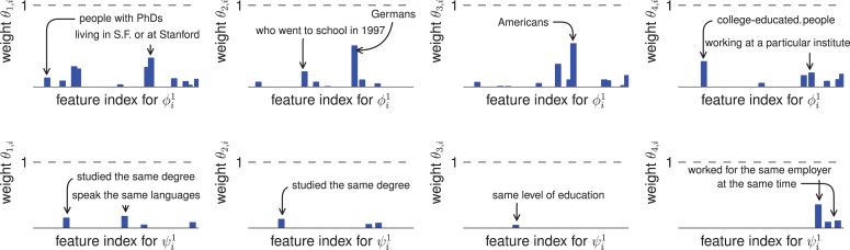
4:6                                                                                  J. McAuley and J. Leskovec

to a value between 0 and 1. This also implicitly defines p(e ∈
                                                             / E). Specifically, we have
                                                    e(e)
                                 p(e ∈ E) =                 ,
                                                  1 + e(e)
                                                                          1
                                 p(e ∈
                                     / E) = 1 − p(e ∈ E) =                       .
                                                                       1 + e(e)
We can now write down the log-likelihood of G:

                     l (G; C) =    (e) −     log(1 + e(e) ).                                                  (3)
                                            e∈E              e∈V ×V

  Next, we describe how to optimize node circle memberships C as well as the param-
eters of the user profile similarity functions  = {(θk, αk)} (k = 1 . . . K) given a graph G
and user profiles.
3. UNSUPERVISED LEARNING OF MODEL PARAMETERS
Treating circles C as latent variables, we aim to find
                                                       ˆ = {θ̂, α̂} to maximize the
regularized log-likelihood of Equation (3):
                                   ˆ Cˆ = argmax l (G; C) − λ (θ ).
                                   ,                                                                            (4)
                                                  ,C

We solve this problem using coordinate ascent on  and C [MacKay 2003]. That is,
we alternate between fitting our latent variables (the circle memberships) and fit-
ting our model parameters (). In practice, the following two steps are iterated until
convergence:
                                          C t = argmax lt (G; C)                                                (5)
                                                        C

                                  t+1 = argmax l (G; C t ) − λ (θ ).                                           (6)


We optimize Equation (6) using L-BFGS, a standard quasi-Newton procedure to opti-
mize smooth functions of many variables [Nocedal 1980]. Computing partial deriva-
tives, we obtain
              ∂l                                 e(e)                   ∂
                  =              −de (k)φ(e)k             +   dk(e)φ(e)k −                                       (7)
              ∂θk                                1+e (e)                  ∂θk
                        e∈V ×V                                   e∈E

               ∂l                                           e(e)
                  =              δ(e ∈
                                     / Ck)φ(e), θk                 −   δ(e ∈
                                                                             / Ck)φ(e), θk.                    (8)
              ∂αk                                           1+e (e)
                        e∈V ×V                                          e∈E

  To optimize Equation (6), we observe that for fixed C\Ci , we can solve
argmaxCi l (G; C \ Ci ) by expressing it as pseudo-boolean optimization in a pairwise
graphical model [Boros and Hammer 2002]. Pseudo-boolean optimization refers to
problems defined over boolean variables. In our setting, we use boolean variables to
define whether or not a node is a member of a particular circle.
  In particular, we will show next that in this context, optimizing the memberships of
a particular circle can be written in the form

                                 argmax        Ei, j (xi , x j ),
                                             X      xi ,x j ∈X

        ACM Transactions on Knowledge Discovery from Data, Vol. 8, No. 1, Article 4, Publication date: February 2014.
Discovering Social Circles in Ego Networks 4:7
where xi and x j are boolean variables, and Ei, j : {0, 1}2 → R is a pairwise energy. This
is the general form of (pairwise) pseudo-boolean optimization, where we optimize a
real-valued objective defined over binary variables. Next, we show that optimizing the
memberships of a single circle can be expressed in this form.
Formally, we find an expression for the conditional log-likelihood of Equation (3),
conditioned on the memberships of nodes to every circle except a particular circle Ck,
and show that it can be written as a sum of pairwise binary energies.
In our setting, binary variables encode the memberships of nodes to a particular
circle Ck. There are four possible cases that we must consider: (1) an edge appears
outside the circle, (2) a nonedge appears outside the circle, (3) an edge appears inside
the circle, and (4) a nonedge appears inside the circle. “Outside the circle” also includes
the case where one of the nodes appears inside the circle but the other does not—that is,
where the pair of nodes “cross” the circle. Intuitively, we want to maximize the energy
and thus cases (2) and (3) should have high energy (we prefer edges inside circles),
whereas (1) and (4) should have low energy (we do not want to many edges outside
the circles). The precise energy should also depend on φ(e), θk, which encodes how
compatible the features of i and j are with the circle’s parameters θk.
In order to achieve this, we first define (for a pair of nodes e)
ok(e) = dk(e)φ(e), θk,
Ci ∈C\Ck
where we are summing over all circles Ci other than the circle Ck whose members
we are currently optimizing. This expression will take a positive value when nodes
at endpoints of edge e = (i, j) belong to many common circles (other than Ck) and a
negative value otherwise.
We then define the pairwise energy Eek (parameterized in terms of the circle k, and a
pair of nodes e = (x, y)) as
ok(e) − αkφ(e), θk − log 1 + eok(e)−αkφ(e),θk , e ∈ E
Eek(0, 0) = Eek(0, 1) = Eek(1, 0) =
−log 1 + eok(e)−αkφ(e),θk , e∈
/E
ok(e) + φ(e), θk − log 1 + eok(e)+φ(e),θk , e ∈ E
Eek(1, 1) = .
−log 1 + eok(e)+φ(e),θk , e∈
/E
Eek(1, 1) corresponds to the case where both nodes belong to the circle, whereas in the
other three cases, at least one node does not belong to the circle. Note that this captures
the four possible cases described earlier (cases 1 through 4 are the four expressions in
the preceding equation, respectively).
Finally, the optimization problem to infer memberships of a single circle becomes
Ck = argmax k
E(x,y) (δ(x ∈ C), δ(y ∈ C)). (9)
C
(x,y)∈V ×V
By expressing the problem in this form, we can draw upon existing work on pseudo-
boolean optimization. Optimization problems of this form are known to be NP-hard
in general, although efficient approximation algorithms are readily available [Rother
et al. 2007]. We use the publicly available QPBO software described in Rother et al.
[2007], which implements algorithms described in Hammer et al. [1984] and Kohli
and Torr [2005] and is able to accurately approximate problems of the form shown in
Equation (9). Essentially, problems of the type shown in Equation (9) are reduced
to maximum flow, where boolean labels for each node are recovered from their as-
signments to “source” and “sink” sets, and the energies E(xi , x j ) are transformed to
ACM Transactions on Knowledge Discovery from Data, Vol. 8, No. 1, Article 4, Publication date: February 2014.4:8 J. McAuley and J. Leskovec
capacities (albeit through a nontrivial transformation). Such algorithms have worst-
case complexity O(|N|3 ), although the average case running time is far better [Kol-
mogorov and Rother 2007]. We solve Equation (9) for each circle Ck in a random order.
The two optimization steps of Equations (5) and (6) are repeated until convergence—
that is, until C t+1 = C t . The entire procedure is presented in Algorithm 1.
Finally, we regularize Equation (4) using the 1 norm,
|θk |
K
(θ ) = |θki |,
k=1 i=1
which leads to sparse (and readily interpretable) parameters.
Our algorithm can readily handle all but the largest problem sizes typically observed
in ego networks: in the case of Facebook, the average ego network has around 190 nodes
[Ugander et al. 2011], whereas the largest network we encountered has 4,964 nodes.
Later, in Section 5, we will exploit the fact that our features are binary, and that many
nodes share similar features, to develop more efficient algorithms based on Markov
Chain Monte Carlo (MCMC) inference. Note that since the method is unsupervised,
inference is performed independently for each ego network. This means that our method
could be run on the full Facebook graph (for example), as circles are independently
detected for each user, and the ego networks typically contain only hundreds of nodes.
In Section 4, we describe extensions that allow our model to be used in semisupervised
settings.
ALGORITHM 1: Predict complete circles with hyperparameters λ, K.
Data: ego-network G = (V, E), edge features φ(e) : E → R F , hyperparameters λ, K
Result: parameters ˆ := {(θ̂k, α̂k)}k=1...K , communities Cˆ
initialize θk0 ∈ {0, 1} F , αk0 := 1, Ck := ∅, t := 0;
repeat
for k ∈ {1 . . . K} do
Ckt := argmaxC (x ,y)∈V ×VE(xk ,y) (δ(x ∈ C ), δ(y ∈ C ));
// using QPBO, see (eq. 9)
end
t+1 := argmax l (G; C t ) − λ (θ);
// using L-BFGS, see (eqs. 7 and 8)
t := t + 1;
until C t+1 = C t ;
3.1. Hyperparameter Estimation
Estimating the number of circles. To automatically choose the optimal number
of circles, we choose K to minimize an approximation to the Bayesian Information
Criterion (BIC), an idea seen in several works on probabilistic clustering [Airoldi et al.
2008; Handcock et al. 2007a; Volinsky and Raftery 2000]. In this context, the BIC is
defined as
BIC(K; K ) −2l K (G; C) + | K | log |E|, (10)
where is the set of parameters predicted when there are K circles, and | | is the
K K
number of parameters (which increases linearly as K increases). We then choose K so
as to minimize this objective:
K̂ = argmin BIC(K; K ). (11)
K
ACM Transactions on Knowledge Discovery from Data, Vol. 8, No. 1, Article 4, Publication date: February 2014.Discovering Social Circles in Ego Networks 4:9
In other words, an additional circle will only be added to the model if doing so has a
significant impact on the log-likelihood.
Regularizer. The regularization parameter λ ∈ {0, 1, 10, 100} was determined using
leave-one-out cross validation, although in our experience, λ did not significantly impact
performance.
4. EXTENSIONS
So far, we have considered the cold-start problem of predicting complete sets of circles
using nothing but node attributes and edge information. In other words, we have
treated circle prediction as an unsupervised task. This setting is realistic if users
construct their circles only after their ego networks have already been defined. On the
other hand, in settings where users build their circles incrementally, it is less likely
that we would wish to predict complete circles from scratch. We note that both settings
occur in the three social networks that we consider.
In this section, we describe techniques to exploit partially observed circle information
to help users update and maintain their circles. In other words, we would like to apply
our model to users’ personal networks as they change and evolve. Since our model is
probabilistic, it is straightforward to adapt it to make use of partially observed data by
conditioning on the assignments of some of the latent variables in our model. In this
way, we adapt our model for semisupervised settings in which a user labels some or
all of the members of their circles. Later, in Section 5, we describe modifications of our
model that allow it to be applied to large networks by exploiting the fact that many
users assigned to common circles also have common features.
4.1. Circle Maintenance
First we deal with the problem of a user adding new friends to an established ego
network, whose circles have already been defined. Thus, given a complete set of circles,
our goal is to predict circle memberships for a new node, based on that node’s features,
and their patterns of connectivity to existing nodes in the ego network.
Our strategy to solve this problem is to adapt our previous algorithms to handle
partially observed data. Rather than estimating circle memberships for all users, we
only estimate the circle memberships of new users while conditioning upon the circle
memberships of existing users.
Since the circles of existing users are fully observed in this setting, we simply fit the
model parameters that best explain the ground-truth circles C¯ provided by the user:
¯ − λ (θ ).
ˆ = argmax l (G; C) (12)
As with Equation (6), this is solved using L-BFGS, although optimization is signifi-
cantly faster in this case, as there are no longer latent community memberships to
infer and thus coordinate ascent is not required.
Next, we must predict to which of the K ground-truth circles a new user u belongs.
That is, we must predict cu ∈ {0, 1} K , where each cku is a binary variable indicating
whether the user u should belong to the circle Ck. In practice, for the sake of evaluation,
we shall suppress a single user from G and C, ¯ and try to recover their memberships.
This can be done by choosing the assignment cu that maximizes the log-likelihood of
C once u is added to the graph. We define the augmented community memberships as
C + (cu) = {Ck+ (cku)}k=1...K , where
C̄k ∪ {u}, cku = 1
Ck+ cku = . (13)
C̄k, cku = 0
ACM Transactions on Knowledge Discovery from Data, Vol. 8, No. 1, Article 4, Publication date: February 2014.4:10 J. McAuley and J. Leskovec
The updated community memberships (for the new node u) are then chosen according
to
ĉu = argmax lˆ (G ∪ {u}; C + (cu)). (14)
cu
The expression presented can be computed efficiently for different values of cu by
noting that the log-likelihood only changes for terms including u, meaning that we need
to compute p((x, y) ∈ E) only if x = u or y = u. In other words, we only need to consider
how the new user relates to existing users rather than considering how existing users
relate to each other; thus, computing the log-likelihood requires linear (rather than
quadratic) time. To find the optimal cu, we can simply enumerate all 2 K possibilities,
which is feasible as long as the user has no more than K 20 circles. For users with
more circles, we must resort to an iterative update scheme as we did in Section 3.
4.2. Semisupervised Circle Prediction
Next we consider the problem of using weak supervision in the form of seed nodes to
assist in circle prediction [Andersen and Lang 2006]. We envision that this version of
the problem could be applied to alleviate the burden of manually labeling circles by
automatically predicting complete circles using a minimal amount of supervision.
Formally, the user manually labels a few users from each of the circles that they want
to create, say {s1 . . . sK }. Our goal is then to predict K circles C = {C1 . . . C K } subject to
the constraint that sk ⊆ Ck for all k ∈ {1 . . . K}.
Again, since our model is probabilistic, this can be done by conditioning on the
assignments of some of the latent variables. That is, we simply optimize l (G; C) subject
to the constraint that sk ⊆ Ck for all k ∈ {1 . . . K}. In the parlance of graphical models,
this means that rather than treating the seed nodes as latent variables to be predicted,
we treat them as evidence on which we condition. We could also include negative
evidence (i.e., the user could provide labels for users who do not belong to each circle),
or we could have users provide additional labels interactively, although the setting
described is the most similar to what is used in practice.
5. FAST INFERENCE IN LARGE EGO NETWORKS
Although our algorithm is able to handle the problem sizes typically encountered in
ego networks (i.e., fewer than 1,000 friends), scalability to larger networks presents
an issue, as we require quadratic memory to encode the compatibility between every
pair of nodes (an issue that we note is also present in the existing approaches that
we consider in Section 8). In this section, we propose a more scalable alternative that
makes use of the fact that many nodes belonging to common communities also share
common features.
Although the model presented in the previous sections allowed for arbitrary feature
vectors, for the scalable version of our algorithm we assume that features φ are binary
valued. We note that the features to be presented in Section 7 satisfy this assumption.
Given that features are binary valued, as are community memberships, if there
are K communities and F-dimensional features, there can be at most 2 K+F types of
node. In other words, every node’s community membership is drawn from {0, 1} K , and
every node’s feature vector is drawn from {0, 1} F , so there are at most 2 K+F distinct
community/feature combinations. Of course, the number of distinct node types is also
bounded by |V |, the number of nodes in the graph.
In practice, however, the number of distinct node types is much smaller, as nodes
belonging to common communities tend to have common features. Community member-
ships are also not independent: in Figure 2, we observed both disjoint and hierarchically
nested communities, which means that of the 2 K possible community memberships,
only a fraction of them occur in practice.
ACM Transactions on Knowledge Discovery from Data, Vol. 8, No. 1, Article 4, Publication date: February 2014.Discovering Social Circles in Ego Networks 4:11
Fig. 2. Histogram of overlap between circles (on Facebook). A value of zero indicates that the circle does
not intersect with any of the user’s other circles, whereas a value of one indicates that a circle is entirely
contained within another. Approximately 25% of circles exhibit the latter behavior.
In this section, we propose an MCMC sampler [Newman and Barkema 1999] that
efficiently updates node-community memberships by “collapsing” nodes that have com-
mon features and community memberships. Note that the adaptations to be described
can be applied to any types of feature (i.e., not just binary features). All we require is
that many users share the same features; we assume binary features merely for the
sake of presentation. Our implementation of these algorithms is available online.1
We start by representing each node using binary strings that encode both its com-
munity memberships and its features. Each node’s community memberships are rep-
resented using S : V → K , such that
1, if x ∈ Ck
S(x)[k] = . (15)
0, otherwise
Similarly, each node’s features are represented using the binary string Q, which, since
our features are already binary, is simply the concatenation of the feature dimensions.
We now say that the type of a node x is the concatenation of its community string
and its feature string, (S(x); Q(x)), and we build a (sparse) table types : K × F → N
that counts how many nodes exist of each type.
In our setting, MCMC consists of repeatedly updating the (binary) label of each node
in a particular community. Specifically, if the marginal (log) probability that a node x
belongs to a community k is given by kx , then the node’s new label is chosen by sampling
z ← U(0, 1), and updating
1, if z < exp T1 kx (1) − kx (0)
S(x)[k] = , (16)
0, otherwise
where T is a temperature parameter that decreases at each iteration so that we are
more likely to choose the label with higher probability as the model “cools.”
Computing kx (0) and kx (1) (the probability that node x takes the label 0 or 1 in
community k) requires computing p((x, y) ∈ E) for all y ∈ V . However, we note that
if two nodes y and y have the same type (i.e., they belong to the same communities
and have the same features), then p((x, y) ∈ E) = p((x, y ) ∈ E). In order to maximize
the log-likelihood of the observed data, we must also consider whether (x, y) and (x, y )
are actually edges in the graph. To do so, we first compute kx (0) and kx (1) under the
assumption that no edges are incident on x, after which we correct for those edges
incident on x. Thus, the running time of a single update is linear in the number of
distinct node types, plus the average node degree, both of which are bounded by the
number of nodes.
1 Stanford Network Analysis Platform: http://snap.stanford.edu/snap.
ACM Transactions on Knowledge Discovery from Data, Vol. 8, No. 1, Article 4, Publication date: February 2014.4:12 J. McAuley and J. Leskovec
ALGORITHM 2: Update memberships node x and circle k.
Data: node x whose membership to circle Ck is to be updated
Result: updated membership for node x
initialize kx (0) := 0, kx (1) := 0;
construct a dummy node x0 with the communities and features of x but with x ∈
/ Ck ;
construct a dummy node x1 with the communities and features of x but with x ∈ Ck;
for (c, f ) ∈ dom(types) do
// c = community string, f = feature string
n := types(c, f );
// n = number of nodes of this type
if S(x) = c ∧ Q(x) = f then
// avoid including a self-loop on x
n := n − 1;
end
construct a dummy node y with community memberships c and features f ;
// first compute probabilities assuming all pairs (x, y) are non-edges
x (0) := x (0) + n log p((x0 , y) ∈ / E);
k k
k
x (1) := k
x (1) + n log p((x 1 , y) ∈
/ E);
end
for (x, y) ∈ E do
// correct for edges incident on x
x (0) := x (0) − log p((x0 , y) ∈ / E) + log p((x0 , y) ∈ E);
k k
x (1) − log p((x1 , y) ∈/ E) + log p((x1 , y) ∈ E);
k k
x (1) :=
end
// update membership to circle k
types(S(x), Q(x)) := types(S(x), Q(x)) − 1;
z ← U(0, 1);
if z < exp {T ( kx (1) − kx (0))} then
S(x)[k] := 1
else
S(x)[k] := 0
end
types(S(x), Q(x)) := types(S(x), Q(x)) + 1;
In terms of Big-O notation, our MCMC algorithm computes updates in worst case
O(|N|2 ) per iteration, whereas our pseudo-boolean optimization algorithm of Section 3
(which is based on maximum flow) requires O(|N|3 ). These are both loose, worst-case
upper bounds: our MCMC algorithm is much faster if many nodes share common
community affiliations, and maximum flow is typically much faster than cubic time.
In practice, our pseudo-boolean optimization procedure is limited by quadratic mem-
ory requirements (energies must be stored for all pairs of nodes); this limitation is
circumvented by our MCMC algorithm.
The entire procedure is demonstrated in Algorithm 2.
We also exploit the same observation when computing partial derivatives of the log-
likelihood—that is, we first efficiently compute derivatives under the assumption that
the graph contains no edges and then correct the result by summing over all edges in
E.
6. DATASET DESCRIPTION
Although our method is unsupervised, we require labeled ground-truth data in order
to evaluate its performance. We expended significant time, effort, and resources to
ACM Transactions on Knowledge Discovery from Data, Vol. 8, No. 1, Article 4, Publication date: February 2014.Discovering Social Circles in Ego Networks 4:13 obtain high-quality hand-labeled data, which we have made available.2–4 We were able to obtain ego networks and ground truth from three major social networking sites: Facebook, Google+, and Twitter. From Facebook, we obtained profile and network data from 10 ego networks, consist- ing of 193 circles and 4,039 users. Data was obtained using a Facebook application.5 To obtain circle information, we developed our own Facebook application and conducted a survey of 10 users (mostly Stanford graduate students), who were asked to manually identify all of the circles to which their friends belonged. It took each user around 2 to 3 hours to label their entire network. On average, users identified 19 circles in their ego networks, with an average circle size of 22 friends. Examples of circles that we obtained include students of common universities and classes, sports teams, relatives, and so forth. Figure 2 shows the extent to which our 193 user-labeled circles in 10 ego networks from Facebook overlap (intersect) with each other. Around one quarter of the identified circles are independent of any other circle, although a similar fraction is completely contained within another circle (e.g., friends who studied under the same advisor may be a subset of friends from the same university). The remaining 50% of communities overlap to some extent with another circle. For the other two datasets, we obtained publicly accessible data. From Google+, we obtained data from 133 ego networks, consisting of 479 circles and 106,674 users. Data was collected from a Web page devoted to maintaining a list of publicly shared circles.6 The Google+ circles are quite different from those from Facebook, in the sense that their creators have chosen to release them publicly, and because Google+ is a directed network (note that our model can very naturally be applied to both to directed and undirected networks). For example, many of our Google+ circles are collections of authors, politicians, or celebrities, who are presumably not close personal friends of the users who follow them. Finally, from Twitter, we obtained data from 1,000 ego networks, consisting of 4,869 circles (or lists [Kim et al. 2010; Nasirifard and Hayes 2011; Wu et al. 2011; Zhao 2011]) and 81,362 users. We started from a single Twitter user and proceeded in a breadth-first-search fashion, collecting data from users who had created at least two lists, stopping once we had 1,000 users. The ego networks that we obtained range in size from 10 to 4,964 nodes. We acknowledge that there may be certain biases in our sample of users from whom we obtain ground truth. Our Facebook users are mostly graduate students, our Google+ users are those who have chosen to release their circles, and so forth. To address this, we are currently involved in a community effort to obtain larger, more representative datasets of the same form.7 Taken together, our data contains 1,143 different ego networks; 5,541 circles; and 192,075 users. The size differences between these datasets simply reflects the avail- ability of data from each of the three sources. Our Facebook data is fully labeled, in the sense that we obtain every circle that a user considers to be a cohesive community, whereas our Google+ and Twitter data is only partially labeled, in the sense that we only have access to public circles. We design our evaluation procedure in Section 8 so that partial labels cause no issues. 2 Facebook: http://snap.stanford.edu/data/egonets-Facebook.html. 3 Google+: http://snap.stanford.edu/data/egonets-Gplus.html. 4 Twitter: http://snap.stanford.edu/data/egonets-Twitter.html. 5 http://snap.stanford.edu/socialcircles/. 6 http://publiccircles.appspot.com/. 7 https://www.kaggle.com/Facebook-Circles. ACM Transactions on Knowledge Discovery from Data, Vol. 8, No. 1, Article 4, Publication date: February 2014.
4:14                                                                                J. McAuley and J. Leskovec

Fig. 3. Feature construction. Profiles are tree structured, and we construct features by comparing paths in
those trees. Examples of trees for two users x (blue) and y (pink) are shown at top. Two schemes for construct-
ing feature vectors from these profiles are shown at bottom. (1) (bottom left) We construct binary indicators
measuring the difference between leaves in the two trees—for example, ‘work→position→Cryptanalyst’ ap-
pears in both trees. (2) (bottom right) We sum over the leaf nodes in the first scheme, maintaining the fact
that the two users worked at the same institution but discarding the identity of that institution.

7. CONSTRUCTING FEATURES FROM USER PROFILES
Profile information in all of our datasets can be represented as a tree where each level
encodes increasingly specific information (Figure 3, left). In other words, user profiles
are organized into increasingly specific categories. For example, a user’s profile might
have an education category, which would be further separated into categories such
as name, location, and type. The leaves of the tree are then specific values in these
categories,such as Princeton, Cambridge, and Graduate School. Several works deal
with automatically building features from tree-structured data [Haussler 1999; Vish-
wanathan and Smola 2002], but in order to understand the relationship between circles
and user profile information, we shall design our own feature representation scheme.
  We propose two hypotheses for how users organize their social circles: either they
may form circles around users who share some common property with each other, or
they may form circles around users who share some common property with themselves.
For example, if a user has many friends who attended Stanford, then they may form a

         ACM Transactions on Knowledge Discovery from Data, Vol. 8, No. 1, Article 4, Publication date: February 2014.
Discovering Social Circles in Ego Networks 4:15
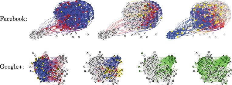
Fig. 4. Features obtained from Facebook. Each of the 26 leaf nodes is one category of features that we
consider. Certain features (e.g., education) may appear multiple times with different values (e.g., for multiple
schools that a user attended).
Stanford circle. On the other hand, if they themselves did not attend Stanford, they may
not consider attendance to Stanford to be a salient feature. The feature construction
schemes that we propose allow us to assess which of these hypotheses better represents
the data we obtain.
From Google+, we collect data from six categories (gender, last name, job titles,
institutions, universities, and places lived). From Facebook, we collect data from 26
categories, including users’ hometowns, birthdays, colleagues, political and religious
affiliations, and so forth. As a proxy for profile data, from Twitter we collect data from
two categories, namely the set of hashtags and mentions used by each user during
2 weeks’ worth of tweets. Categories correspond to parents of leaf nodes in a profile
tree, as shown in Figure 3. The full set of features that we obtain from Facebook is
shown in Figure 4.
We first propose a difference vector to encode the relationship between two profiles.
A nontechnical description is given in Figure 3. Essentially, we want to encode those
dimensions where two users are the same (e.g., Alan and Dilly went to the same
graduate school) and those where they are different (e.g., they do not have the same
surname). Suppose that users v ∈ V each have an associated profile tree Tv and that
l ∈ Tv is a leaf in that tree. We define the difference vector σx,y between two users x
and y as a binary indicator encoding the profile aspects where users x and y differ
(Figure 3, bottom left):
σx,y [l] = δ((l ∈ Tx ) = (l ∈ T y )). (17)
Note that feature descriptors are defined per ego network: although many thousands of
high schools (for example) exist among all Facebook users, only a small number appear
among any particular user’s friends.
Although the difference vector presented has the advantage that it encodes profile
information at a fine granularity, it has the disadvantage that it is high dimensional
(up to 4,122 dimensions in the data we considered). One way to address this is to form
difference vectors based on the parents of leaf nodes: this way, we encode what profile
categories two users have in common but disregard specific values (Figure 3, bottom
right). For example, we encode how many hashtags two users tweeted in common, but
we discard which hashtags they tweeted:
σx,y [ p] = σx,y [l]. (18)
l∈ children( p)
ACM Transactions on Knowledge Discovery from Data, Vol. 8, No. 1, Article 4, Publication date: February 2014.4:16 J. McAuley and J. Leskovec
This scheme has the advantage that it requires a constant number of dimensions
regardless of the size of the ego network (26 for Facebook, 6 for Google+, 2 for Twitter,
as described earlier).
Based on the difference vectors σx,y (and σx,y ), we now describe how to construct edge
features φ(x, y). The first property we wish to model is that members of circles should
have common relationships with each other:
φ 1 (x, y) = (1; −σx,y ). (19)
The second property we wish to model is that members of circles should have common
relationships to the ego of the ego network. In this case, we consider the profile tree Tu
from the ego user u. We then define our features in terms of that user:
φ 2 (x, y) = (1; −|σx,u − σ y,u|) (20)
(|σx,u − σ y,u| is taken elementwise). These two parameterizations allow us to assess
which mechanism better captures users’ subjective definition of a circle. In both cases,
we include a constant feature (“1”), which controls the probability that edges form
within circles, or equivalently it measures the extent to which circles are made up of
friends. Importantly, this allows us to predict memberships even for users who have no
profile information, simply due to their patterns of connectivity.
Similarly, for the “compressed” difference vector σx,y , we define
ψ 1 (x, y) = (1; −σx,y ), ψ 2 (x, y) = (1; −|σx,u − σ y,u |). (21)
To summarize, we have identified four ways of representing the compatibility between
different aspects of profiles for two users. We considered two ways of constructing a
difference vector (σx,y vs. σx,y ) and two ways of capturing the compatibility between a
pair of profiles (φ(x, y) vs. ψ(x, y)). These features are designed to model the following
behavior:
(1) Ego users build circles around common relationships between their friends (φ 1 ,
ψ 1 ).
(2) Ego users build circles around common relationships between their friends and
themselves (φ 2 , ψ 2 ).
In our experiments, we assess which of these assumptions is more realistic in practice.
8. EXPERIMENTS
We first describe the evaluation metrics to be used in Sections 8.1 and 8.2, before
describing the baselines to be evaluated in Section 8.4. We describe the performance of
our (unsupervised) algorithm in Section 8.5 and extensions in Sections 8.7, 8.8, and 8.9.
8.1. Evaluation Metrics
Although our method is unsupervised, we can evaluate it on ground-truth data by
examining the maximum-likelihood assignments of the latent circles C = {C1 . . . C K }
after convergence. Our goal is that for a properly regularized model, the latent circles
will align closely with the human-labeled ground-truth circles C¯ = {C̄1 . . . C̄ K̄ }.
To measure the alignment between a predicted circle C and a ground-truth circle
C̄, we compute the Balanced Error Rate (BER) between the two circles [Chen and Lin
2006],
1 |C\C̄| |C c \C̄ c |
BER(C, C̄) = + . (22)
2 |C| |C c |
ACM Transactions on Knowledge Discovery from Data, Vol. 8, No. 1, Article 4, Publication date: February 2014.Discovering Social Circles in Ego Networks 4:17
This measure assigns equal importance to false positives and false negatives so that
trivial or random predictions incur an error of 0.5 on average. Such a measure is
preferable to the 0/1 loss (for example), which assigns extremely low error to trivial
predictions. We also report the F1 score:
precision(C, C̄) · recall(C, C̄)
F1 (C, C̄) = 2 · . (23)
precision(C, C̄) + recall(C, C̄)
Treating C̄ as a set of “relevant” documents, and C as a set of “retrieved” documents,
precision and recall are defined as
|C ∩ C̄| |C ∩ C̄|
precision(C, C̄) = , recall(C, C̄) = . (24)
|C| |C̄|
In practice, we find that the BER and the F1 score product qualitatively similar results.
The preceding scores compare a single predicted circle C to a single ground-truth circle
¯
C̄. Next we describe how we compute the error for sets of circles C and C.
8.2. Aligning Predicted and Ground-Truth Circles
¯ we compute the
Since we do not know the correspondence between circles in C and C,
optimal match via linear assignment by maximizing:
1
max (1 − BER(C, f (C))), (25)
f :C→C¯ | f|
C∈dom( f )
where f is a (partial) correspondence between C and C. ¯ That is, if the number of
predicted circles |C| is less than the number of ground-truth circles |C|,¯ then every
circle C ∈ C must have a match C̄ ∈ C, ¯ but if |C| > |C|,
¯ we do not incur a penalty for
additional predictions that could have been circles but were not included in the ground
truth. We use established techniques to estimate the number of circles so that none of
the baselines suffers a disadvantage by mispredicting K̂ = |C|. Similarly, when using
the F1 score, we compute the optimal match by maximizing:
1
max F1 (C, f (C)). (26)
f :C→C¯ | f |
C∈dom( f )
The preceding loss is designed to be insensitive to the fact that we have incomplete
ground truth. That is, we allow for the possibility that we obtain only some of each
user’s possible circles. However, in the case of Facebook (where we have “complete”
ground truth in the sense that survey participants ostensibly label every circle), our
method should penalize predicted circles that do not appear in the ground truth. A
simple penalty would be to assign an error of 0.5 (i.e., that of a random prediction)
to additional circles in the case of Facebook. However, in our experience, our method
did not overpredict the number of circles in the case of Facebook: on average, users
identified 19 circles, whereas using the BIC described in Section 3.1, our method never
predicted K > 10. In practice, this means that in the case of Facebook, we always
penalize all predictions. Again we note that the process of choosing the number of
circles using the BIC is a standard procedure from the literature [Airoldi et al. 2008;
Handcock et al. 2007a; Volinsky and Raftery 2000], whose merit we do not assess in
this article.
ACM Transactions on Knowledge Discovery from Data, Vol. 8, No. 1, Article 4, Publication date: February 2014.4:18 J. McAuley and J. Leskovec
8.3. Estimating the Number of Circles for Nonprobabilistic Baselines: Network Modularity
Although for our algorithm, and other probabilistic baselines, we shall choose the
number of communities using the BIC as described in Section 3.1, another standard
criterion used to determine the number of communities in a network is the modularity
[Newman 2006].
The BIC has the advantage that it allows for overlapping communities, whereas the
modularity does not (i.e., it assumes all communities are disjoint); it is for this reason
that we chose the BIC to choose K̂ for our algorithm. On the other hand, the BIC can
only be computed for probabilistic models (i.e., models that associate a likelihood with
each prediction), whereas the modularity has no such restriction. For this reason, we
shall use the modularity to choose K̂ for nonprobabilistic baselines.
The modularity essentially measures the extent to which clusters in a network have
dense internal, but sparse external, connections [Newman 2003]. If ei j is the fraction of
edges in the network that connect vertices in Ci to vertices in C j , then the modularity
is defined as
⎧ ⎫
K ⎨
K ⎬
Q(K) = eii − ei j . (27)
⎩ ⎭
i=1 j=1
We then choose K̂ so that the modularity is maximized.
8.4. Baselines
We considered a wide number of baseline methods, including those that consider only
network structure, those that consider only profile information, and those that consider
both.
Mixed Membership Stochastic Block Models [Airoldi et al. 2008]. This method
detects communities based only on graph structure; the output is a stochastic vector
for each node encoding partial memberships to each community. The optimal number
of communities K̂ is determined using the BIC as described in Equation (11). This
model is similarto those of Liu et al. [2009] and Chang and Blei [2009], the latter of
which includes the implementation of MMSB that we used. Since we require “hard”
memberships for evaluation, we assign a node to a community if its partial membership
to that community is positive.
Block-LDA [Balasubramanyan and Cohen 2011]. This method is similar to MMSB,
except that it allows nodes to be augmented with side information in the form of
“documents.” For our purposes, we generate documents by treating aspects of user
profiles as words in a bag-of-words model.
K-means Clustering [MacKay 2003]. Just as MMSB uses only the graph structure,
K-means clustering ignores the graph structure and uses only node features (for node
features, we again use a bag-of-words model). Here we choose K̂ to maximize the
modularity of C, as defined in Equation (27).
Hierarchical Clustering [Johnson 1967]. This method builds a hierarchy of clus-
ters. Like K-means, this method forms clusters based only on node profiles but ignores
the network.
Link Clustering [Ahn et al. 2010]. Conversely, this method uses network structure
but ignores node features to construct hierarchical communities in networks.
Clique Percolation [Palla et al. 2005]. This method also uses only network
structure and builds communities from the union of small, densely connected
subcommunities.
Low-Rank Embedding [Yoshida 2010]. This method uses both graph structure and
node similarity information but does not perform any learning. We adapt an algorithm
ACM Transactions on Knowledge Discovery from Data, Vol. 8, No. 1, Article 4, Publication date: February 2014.You can also read