Comparison of Spectral Reflectance-Based Smart Farming Tools and a Conventional Approach to Determine Herbage Mass and Grass Quality on Farm - MDPI
←
→
Page content transcription
If your browser does not render page correctly, please read the page content below
remote sensing
Article
Comparison of Spectral Reflectance-Based Smart
Farming Tools and a Conventional Approach to
Determine Herbage Mass and Grass Quality on Farm
Leonie Hart 1,2, *, Olivier Huguenin-Elie 3 , Roy Latsch 1 , Michael Simmler 1 ,
Sébastien Dubois 4 and Christina Umstatter 1
 1    Competitiveness and System Evaluation, Agroscope, Tänikon 1, 8356 Ettenhausen, Switzerland;
      roy.latsch@bluewin.ch (R.L.); michael.simmler@agroscope.admin.ch (M.S.);
      christina.umstaetter@agroscope.admin.ch (C.U.)
 2    Institute of Agricultural Sciences in the Tropics, University of Hohenheim, Fruwirthstrasse 31,
      70599 Stuttgart, Germany
 3    Animal Production Systems and Animal Health, Agroscope, Reckenholzstrasse 191, 8046 Zurich,
      Switzerland; olivier.huguenin@agroscope.admin.ch
 4    Methods Development and Analytics, Agroscope, Rte de la Tioleyre 4, 1725 Posieux, Switzerland;
      sebastien.dubois@agroscope.admin.ch
 *    Correspondence: leonie.hart@agroscope.admin.ch; Tel.: +41-5-8480-3131

 Received: 11 September 2020; Accepted: 2 October 2020; Published: 7 October 2020

 Abstract: The analysis of multispectral imagery (MSI) acquired by unmanned aerial vehicles (UAVs)
 and mobile near-infrared reflectance spectroscopy (NIRS) used on-site has become increasingly
 promising for timely assessments of grassland to support farm management. However, a major
 challenge of these methods is their calibration, given the large spatiotemporal variability of grassland.
 This study evaluated the performance of two smart farming tools in determining fresh herbage mass
 and grass quality (dry matter, crude protein, and structural carbohydrates): an analysis model for
 MSI (GrassQ) and a portable on-site NIRS (HarvestLabTM 3000). We compared them to conventional
 look-up tables used by farmers. Surveys were undertaken on 18 multi-species grasslands located on
 six farms in Switzerland throughout the vegetation period in 2018. The sampled plots represented
 two phenological growth stages, corresponding to an age of two weeks and four to six weeks,
 respectively. We found that neither the performance of the smart farming tools nor the performance
 of the conventional approach were satisfactory for use on multi-species grasslands. The MSI-model
 performed poorly, with relative errors of 99.7% and 33.2% of the laboratory analyses for herbage mass
 and crude protein, respectively. The errors of the MSI-model were indicated to be mainly caused by
 grassland and environmental characteristics that differ from the relatively narrow Irish calibration
 dataset. The On-site NIRS showed comparable performance to the conventional Look-up Tables in
 determining crude protein and structural carbohydrates (error ≤ 22.2%). However, we identified that
 the On-site NIRS determined undried herbage quality with a systematic and correctable error. After
 corrections, its performance was better than the conventional approach, indicating a great potential
 of the On-site NIRS for decision support on grazing and harvest scheduling.

 Keywords: evaluation; grassland assessment; mobile NIRS; multispectral imagery; UAV

1. Introduction
     For many years, indoor housing has been preferred by dairy producers because feeding and
caretaking on an individual animal level was simpler and more labor-saving compared to grazing-based
systems [1,2]. Currently, due to modern technology that addresses both labor requirements and

Remote Sens. 2020, 12, 3256; doi:10.3390/rs12193256                        www.mdpi.com/journal/remotesensing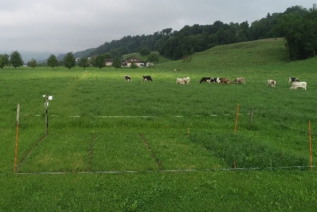
Remote Sens. 2020, 12, 3256                                                                          2 of 19

precision feed supply on pastures, grazing-based dairy production systems are viable again [3,4].
In grazing-based production systems, knowing herbage quantity and quality is key to an efficient use
of the grassland resource because it enables defining adequate stocking rates, optimizing grazing and
harvest scheduling, and refining herbage feeding and concentrate supplementation [5,6].
     In Switzerland, the rate of grass growth varies widely within each growing season and between
years [7]. Moreover, the range of pedoclimatic conditions, topographies, and expositions under which
grasslands are used for forage production is vast. Correspondingly, the spatial variability of grassland
yield is very large [8]. As it is time-consuming to accurately measure herbage growth or grassland
yields, farmers usually settle for a rough estimation. Many farmers estimate standing herbage mass
from visual observation or increasingly by means of a rising plate meter [9]. To accurately estimate
herbage mass, the rising plate meter requires labor-intensive re-calibration for assessing the specific
plots [5], which leads to a trade-off between labor costs and accuracy. Rising plate meters are, moreover,
only suited for measuring low grasslands in the early growth stages [9].
     The quality of herbage as livestock feed is also widely variable. The quality highly depends on
the growth stage, and thus, on the timing of cutting and grazing [10]. Furthermore, the quality is
subjected to large seasonal variability [6] and is influenced by the weather conditions that prevail
during the weeks preceding harvesting [11]. Moreover, the plant species composition is also an
important influential factor [12]. On commercial farms, herbage quality is rarely determined, as no
convenient method is available. Obtaining accurate information about herbage quality by means
of laboratory analyses requires proper, representative herbage sampling, which is a difficult task at
farm scale. Moreover, the high cost and latency until delivery of the results often render laboratory
analyses unsuitable for farmers because decisions, such as time of meadow harvest, are made short
term, depending on the weather forecast.
     A conventional alternative to laboratory analyses is to visually assess the grassland in the field and
determine herbage quality based on look-up tables, such as the look-up tables by Daccord et al. [10] for
Swiss grasslands. The reference values by Daccord et al. [10] consider important influencing factors.
Pure stands and seven types of multi-species grasslands are distinguished according to their botanical
composition, and five growth stages are differentiated. Quality is assumed to be constant over the year,
apart from differentiating the first growth and the subsequent regrowth [10]. An advantage of such
reference values is that they enable farmers to obtain a real-time rough estimate of herbage quality.
A disadvantage is that this method requires the farmer to determine the growth stage and grassland
botanical composition, which is a challenging task for multi-species grasslands [13]. An obvious
disadvantage is furthermore that look-up tables cannot capture the full natural variation as only a
limited number of sward characteristics are included.
     In overcoming the limitations of the conventional methods, such as the use of rising plate-meters
and look-up tables, spectral reflectance-based smart farming tools might play a major role. With
spectral reflectance analysis, the biomass and quality of herbaceous matter is determined based on
the spectral signature of the material [14,15]. One commonly employed method is near-infrared
reflectance spectroscopy (NIRS), which was proposed for quality measurements of animal feed in the
1970s [16]. Since then, several calibration studies were undertaken to determine the characteristics
and nutrient concentrations in herbage, haylage, and grass silage [17–20]. NIRS instruments can
accurately measure these feed quality features when used under laboratory conditions on dried and
milled samples, given an adequate calibration dataset [21]. In recent years, NIR spectrometers were
integrated into smart-farming tools that directly analyze fresh herbage without prior drying and
milling of a sample. These tools are available as portable laboratories to work on-site or are mounted
onto harvest machinery to measure in real time (HarvestLabTM 3000, Deere & Company, Moline, IL,
USA; AgriNIR, Dinamica Generale, Poggio Rusco, Italy; Moisture TrackerTM , Digi-Star, Fort Atkinson,
WI, USA; Polytec NIRS, Haldrup, Ilshofen, Germany; NIR4 Farm, Aunir, UK). With portable NIRS
instruments, it is a major challenge to achieve the same level of accuracy as laboratory NIRS [19,22,23].
The difficulty in analyzing field-fresh matter without prior drying and milling is that the heterogeneity
Remote Sens. 2020, 12, 3256 3 of 19
of the plant material, its particle size, and the moisture content affect the light reflectance [19,21].
The spectral signature of water can mask signals, which are important for the quantification of dry
matter quality parameters, such as crude protein concentration [15,24].
Methods that are based on remote sensing are recent alternatives to NIRS for estimating herbage
mass and quality of grassland [25–28]. Most of these methods use multispectral imagery collected
from satellites or unmanned aerial vehicles [26,29]. Analyzing grasslands with remote sensing is
particularly promising because it is non-destructive, can potentially capture large areas, and resolves
spatial variability typically better than methods based on point sampling. Unfortunately, multispectral
imagery only captures the surface of the vegetation with limited information on the subjacent
material. Estimating grassland properties from multispectral imagery might, therefore, be error-prone,
particularly for high-biomass swards [26].
Both NIRS and multispectral imaging methods indirectly determine herbage quantity and quality
and require calibration against a reference method, such as oven-drying or wet chemical analysis.
However, the calibrations need to cover a large heterogeneity in grassland types and a large variability
of grassland conditions during the vegetation period to establish high accuracy. If calibrations are
applied to grassland types and conditions not included in the training data set, it is not always
applicable to generalize the results.
The aim of this study was to evaluate two spectral-reflectance-based smart farming tools for
determining herbage mass and quality of multi-species grasslands—a portable NIRS and a model
to analyze multispectral imagery—and to compare them to the conventional approach of estimating
herbage quality with look-up tables. Using grasslands of contrasting botanical composition and
multiple harvests during the whole vegetation period, the accuracy of the tools by comparison with
laboratory measurements was examined. Further, the relationships between the apparent errors and
the grassland characteristics were investigated to identify potential causes. The smart farming tools
were put into context with the conventional approaches for assessing grassland quality.
2. Materials and Methods
2.1. Experiments
2.1.1. Grassland Study Sites
Herbage mass and quality parameters were measured on 18 grassland plots, which were distributed
over six commercial farms in Switzerland. The studied grasslands are described in Figure 1 and
Table S1. Prior to this study, the grasslands were used for intensive silage or hay production, with four
to six defoliations per year and regular fertilization. With the exception of two grasslands, they were
permanent grasslands that were sown less than five years ago (MT3 and SI2, Table S1). The plant
communities comprised between 13 and 27 species (Table S1), with relative abundances of 6–75%
ryegrasses, 13–59% other grasses, 1–15% clover species, and 2–48% herbs (Figure 1).Remote Sens. 2020, 12, 3256 4 of 19
Remote Sens. 2020, 12, x FOR PEER REVIEW 4 of 20
Remote Sens. 2020, 12, x FOR PEER REVIEW 4 of 20
Figure
Figure 1. Relative
Relative abundance
abundance of of ryegrasses,
ryegrasses, other
other grasses,
grasses, and
and clover
clover and
and herbs
herbs in
in the
the 18 studied
grasslands, which were
grasslands, which weredistributed
distributedoverover
sixsix commercial
commercial farms
farms (MT,(MT, BL,MB,
BL, SB, SB, BB,
MB,andBB,SI).
and SI).
The The
values
values
are theare the average
average values values
from thefrom the botanical
botanical surveyssurveys in and
in spring spring
lateand late summer
summer 2018. 2018.
2.1.2. Experimental Design
On each commercial farm, three plots were distributed spatially over the intensively managed
grassland area of the farms. On each plot, measurements were performed on two different subplots
with dimensions of 2.2 m × 5.0 m (Figure 2). On the two subplots, we simulated two different defoliation
regimes, which correspond to intensive grazing conditions and silage production. The first subplot,
simulating grazing conditions, was defoliated every two to three weeks, at an early phenological
stage. Sampling was conducted every second defoliation and always at an age of two weeks. The
second subplot, simulating silage production, was defoliated every four to six weeks. The defoliation
dates corresponded with the sampling dates. These dates were scheduled to meet the early heading
phenological stage; thus, a more mature stage compared to the grazing simulation. The dates of
Figure 1. Relative abundance of ryegrasses, other grasses, and clover and herbs in the 18 studied
defoliation, therefore, differed among farms according to the climatic conditions of the sites. Therefore,
grasslands, which were distributed over six commercial farms (MT, BL, SB, MB, BB, and SI). The
the two defoliation regimes are subsequently referred to as “two weeks of growth” for simulated
values are the average values from the botanical surveys in spring and late summer 2018.
grazing conditions and (a)“four to six weeks of growth” for the silage production (b) system.
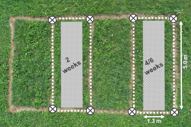
Figure 2. Selected experimental plot, shown as (a) front view and (b) aerial view, where the dashed
lines indicate the two subplots. The sampling areas are highlighted with a checkered pattern. The age
of the herbage at sampling was two weeks (left subplot) and four to six weeks (right subplot). The
ground control points are highlighted as crossed circles.
Both defoliation regimes were planned to be observed on five dates each within the vegetation
period. Therefore, we aimed for a total number of 180 observations. However, due to a severe drought
during summer and autumn, herbage growth was reduced, and three sampling dates had to be
omitted at farms BL and BB. Hence, we obtained a total of 162 herbage samples.
All sampling dates were subsequently assigned to one of the four categories to study the effect
of the growth period on herbage mass and quality: April to May (representing the first regrowth after
winter dormancy), May to June (representing the second cut), June to August (representing the third
(a) to October (representing the fourth and fifth(b)
and fourth cuts), and August cuts).
Figure 2. Selected experimental plot, shown as (a) front view and (b) aerial view, where the dashed
2.1.3.Figure 2. Selected
Herbage Samplingexperimental plot, shown as (a) front view and (b) aerial view, where the dashed
lines indicate
lines indicate the
the two
twosubplots.
subplots.The
Thesampling
samplingareas
areasare
arehighlighted
highlightedwith a checkered
with a checkered pattern. The
pattern. age
The of
age
To
the sample
herbage the
at subplots
sampling with
was twothe four-
weeks to
(left six-week
subplot) old
and herbage,
four to six a double-knife
weeks (right motor
subplot). The
of the herbage at sampling was two weeks (left subplot) and four to six weeks (right subplot). The
mower
ground was
used ground
to cut the
control herbage
points are at 5 cm
highlightedabove-ground,
as crossed and
circles. fresh
control points are highlighted as crossed circles. herbage mass (HM) of 6.5 m 2 (central 1.3 m
of the 2.2 m wide subplots × 5 m) was determined (Figure 2). A representative sample was taken by
stabbing
Bothadefoliation
metal cylinder withwere
regimes a diameter of to
planned 5 cm
be into the pile
observed onof cutdates
five herbage.
each within the vegetation
period. Therefore, we aimed for a total number of 180 observations. However, due to a severe drought
during summer and autumn, herbage growth was reduced, and three sampling dates had to be
omitted at farms BL and BB. Hence, we obtained a total of 162 herbage samples.Remote Sens. 2020, 12, 3256 5 of 19
Both defoliation regimes were planned to be observed on five dates each within the vegetation
period. Therefore, we aimed for a total number of 180 observations. However, due to a severe drought
during summer and autumn, herbage growth was reduced, and three sampling dates had to be omitted
at farms BL and BB. Hence, we obtained a total of 162 herbage samples.
All sampling dates were subsequently assigned to one of the four categories to study the effect of
the growth period on herbage mass and quality: April to May (representing the first regrowth after
winter dormancy), May to June (representing the second cut), June to August (representing the third
and fourth cuts), and August to October (representing the fourth and fifth cuts).
2.1.3. Herbage Sampling
To sample the subplots with the four- to six-week old herbage, a double-knife motor mower was
used to cut the herbage at 5 cm above-ground, and fresh herbage mass (HM) of 6.5 m2 (central 1.3 m
of the 2.2 m wide subplots × 5 m) was determined (Figure 2). A representative sample was taken by
stabbing a metal cylinder with a diameter of 5 cm into the pile of cut herbage.
For the first sampling of the two-week-grown herbage, the same method was applied as described
above. For the subsequent sampling dates, a randomly selected 1 m2 area of the subplot was sampled
at 5 cm above-ground with an electronic hand shear (2 m2 were sampled in case of very low HM).
Fresh HM was determined, and the whole sample was used for further analyses.
2.2. Smart Farming Tools
2.2.1. Multispectral Imagery Model
The multispectral imagery model (MSI-model) was provided on the open access platform GrassQ
(www.grassq.com). According to Murphy et al. [30], GrassQ is a holistic precision herbage measurement
and analysis system that analyzes the reflectance data captured by unmanned aerial vehicles (UAVs)
or satellites above grasslands on a farm parcel level in nearly real time. For this study, the platform
was employed between 2 January 2019 and 2 July 2019. The MSI-model development was based on
data of UAV surveys above field plots and grazed paddocks containing mainly perennial ryegrass and
clover mixtures at Moorepark (Teagasc Research Centre, Fermoy, Cork, Ireland) on six days in 2017
and 2018 [31]. The calibration range for HM is 304.6 to 2435.7 kg dry matter (DM) ha−1 and for crude
protein (CP) 126.3 to 247.3 g kg−1 DM. The models were derived by stepwise multiple linear regression
analysis and are referred to as BM-5 and CPM-5 in Askari et al. [31].
In this study, we chose comparable flight characteristics and used the same sensor utilized by
Askari et al. [31]. MSI was acquired two hours before cutting the subplots at maximum. We used a
Parrot Sequoia multispectral camera (Parrot SA, Paris, France) that was mounted on a UAV (quadcopter,
DJI Phantom 4 Pro+, DJI, Shenzhen, China). Both a sequoia sunshine sensor and a calibrated reference
panel (Airinov, Paris, France) were employed for radiometric correction. Images were taken during
autonomous flights over the experimental plots. The flight missions were planned in the field using the
smart device App Pix4D Capture (Version 4.5.0, build 2348, Pix4D, Lausanne, Switzerland). The flight
and imagery settings were as follows: flight height of 50 m, flight speed of 5 m s−1 , double grid mission,
image capturing every 1.9 s, and image overlap of ≥ 80%. Spectral information was recorded for the
green, red, red-edge, and near-infrared (NIR) bands that were centered at 550 nm, 660 nm, 735 nm, and
790 nm, respectively. The bandwidth was 40 nm, except for the red-edge, which had a bandwidth of
10 nm. The average ground sampling distance was 5 cm. Due to dense fog and rainy weather, images
could not be taken at three sampling dates. Additional data points were not considered for analysis
because of the low image quality, resulting in 15 excluded and 147 remaining MSI data points.
The raw MSI was processed with the photogrammetry software Pix4D Mapper with default
settings and radiometric correction based on reference panel images (Version 4.3.31, Pix4D, Lausanne,
Switzerland). The resulting reflectance maps were georeferenced using at least three of the eight ground
control points at each experimental plot (Figure 2), which were measured using a real-time kinematicRemote Sens. 2020, 12, 3256 6 of 19
global navigation satellite system (RTK GNSS), Trimble R8, Sunnyvale, CA, USA). After georeferencing,
the absolute horizontal accuracy of the reflectance maps was less than 6 cm. The reflectance maps of the
four bands (green, red, red-edge, and NIR) were uploaded to the GrassQ platform (www.grassq.com),
and the model that uses UAV-acquired MSI reflectance maps was executed (hereafter referred to as
MSI-model). The CP results (as g kg−1 DM) and HM results (as kg DM ha−1 ) were given as mean values
per subplot by the MSI-model, which we extracted by uploading the spatial boundary coordinates.
2.2.2. On-Site NIRS
The portable NIRS instrument (HarvestLabTM 3000, Deere & Company, Moline, IL, USA), hereafter
referred to as On-site NIRS, can be operated as a mobile laboratory either in farm offices or car boots
or mounted onto harvest machinery to analyze feed quality in the field and in nearly real time.
The instrument consisted of a sensor body with the diode array spectrometer and a sampling unit with
a rotating sampling dish above a halogen light source. The system operated with internal black and
white references and measured wavelengths between 950 nm and 1530 nm at a spectral resolution
of 3–2 nm. Selectable calibration models were available for different fodder crops. We evaluated the
system for measuring fresh herbage quality using the calibration version 2017/21/03. The instrument
was delivered and put into operation by a service technician approximately six weeks before the start
of the study. The calibration models, therefore, were based on the reference methods described in
VDLUFA [32] and were analog to the wet-chemical analyses in our study. During field sampling,
fresh herbage was analyzed using the On-site NIRS in the open boot of a car. The measurement was
performed immediately after herbage sampling as described above. Due to the missing manufacturer’s
specifications, a particle length of approximately 5 cm was chosen and obtained by stabbing with a
metal cylinder. A representative part of the sampled herbage was filled in the instruments’ sampling
dish. Care was taken to assure that the sampling dish was clean and dry. The measurement was
repeated three times with mixing of the subsample in between. Mean values of DM concentration and
mean values of CP, crude fiber (CF), acid detergent fiber (ADF), and neutral detergent fiber (NDF) as
concentrations of DM were recorded.
2.3. Conventional Method
Additional to the two smart farming tools, the herbage quality parameters (DM, CP, CF, ADF,
and NDF) were determined by using look-up tables for herbage quality of multi-species grasslands by
Daccord et al. [10], hereafter referred to as Look-up Tables. For this reason, the number and relative
abundance of plant species were visually surveyed in April/May and a second time in July/August.
The average of both surveys was used to determine the herbage categories according to Table 13.1 in
Daccord et al. [10], where the seven categories distinguish between grass-rich, legume-rich, herb-rich,
and grass-legume-herb-balanced multi-species grasslands. At the first sampling date in spring, the
phenological stage was determined by direct visual observation. The following determinations of the
phenological stage were performed using Table 13.2 in Daccord et al. [10], considering the time period
since last defoliation.
2.4. Laboratory Analysis
The herbage samples were oven-dried at 60 ◦ C for 48 h and weighed to determine DM as a
percentage of fresh matter (FM). The HM in kg DM ha−1 was calculated for each subplot based on the
area that was cut and weighed during field sampling. A dried subsample was milled to pass a 1 mm
sieve (Brabender, Duisburg, Germany). Between 100 g and 200 g of a milled sample were analyzed
using a laboratory NIRS measuring wavelengths in the range of 1000–2500 nm at a spectral resolution
of 8 cm−1 (Fourier-transform NIR; NIRFlex N-500 system; Büchi, Flawil, Switzerland). The calibration
model for CP, CF, NDF, and ADF is shown in Table S2. The laboratory NIRS was used as a reference
method to evaluate the performance of the herbage quality determination by the On-site NIRS and the
MSI-model (Table 1).Remote Sens. 2020, 12, 3256 7 of 19
Table 1. Evaluated smart farming tools and determined herbage parameters with the respective
reference methods.
Measurement Tools Measured Herbage
Sensing Method Reference Methods
(Number of Samples) Parameters [Unit]
MSI-model MSI of the bands green, HM [kg DM ha−1 ] Cutting defined area + oven-drying
(n = 147) red, red-edge, and NIR CP [g kg−1 DM] Laboratory NIRS
DM [g kg−1 FM] Oven-drying
CP [g kg−1 DM] Laboratory NIRS
On-site NIRS
(n = 162)
NIRS with diode array CF [g kg−1 DM] Laboratory NIRS
NDF [g kg−1 DM] Laboratory NIRS
ADF [g kg−1 DM] Laboratory NIRS
MSI: multispectral imagery; NIRS: near-infrared reflectance spectroscopy; NIR: near-infrared; HM: herbage mass;
DM: dry matter; FM: fresh matter; CP: crude protein; CF: crude fiber; NDF: neutral detergent fiber; ADF: acid
detergent fiber.
To validate the laboratory NIRS, a milled subsample of one third of the herbage samples was
subjected to wet-chemical analyses. The selected samples covered all farms and sampling dates and
represented the observed variation in herbage composition well (Table S1). The DM determination was
based on ISO 6496:1999 with the following modifications: 1–2 g of sample were heated in a prepASH
system (Precisa instruments AG, Dietikon, Switzerland) at 105 ◦ C for 3 h to reach constant weight.
The CP was determined using the Dumas method (ISO 16634-1:2008), and CF was analyzed based
on ISO 6865:2000 with the modifications that 0.5 g of the sample were treated in a FIBRETHERM
FT12 system (C. Gerhardt GmbH & Co. KG, Königswinter, Germany). The concentration of ADF and
NDF were measured using the FT12 system following the methods AOAC 973.18 and ISO 16472:2006,
respectively, and expressed based on the organic matter content (ash-free dry weight). Prior to the
NDF determination, the sample was treated with a heat stable amylase. Table 2 gives an overview of
the wet chemical methods that were used to validate the laboratory NIRS herbage parameters.
Table 2. Herbage parameters determined by the laboratory NIRS with the respective wet-chemical
methods for validation.
Measurement System Measured Herbage
Sensing Method Validation Methods
(Number of Samples) Parameters [Unit]
CP [g kg−1 DM] Dumas method
Laboratory NIRS CF [g kg−1 DM] Gravimetric analysis
Fourier-transform NIRS
(n = 54) NDF [g kg−1 DM] Gravimetric analysis
ADF [g kg−1 DM] Gravimetric analysis
NIRS: near-infrared reflectance spectroscopy; DM: dry matter; CP: crude protein; CF: crude fiber; NDF: neutral
detergent fiber; ADF: acid detergent fiber.
2.5. Statistical Analysis
Agreement of the On-site NIRS and the MSI-model with the reference methods was assessed
with Lin’s concordance correlation coefficient (CCC) [33], which ranges from −1 to +1. CCC considers
both the linear correlation between the methods and the distance between the line of best fit to the
line of identity (1:1 line). Agreement was considered negligible (x ≤ 0.30), slight (0.30 < x ≤ 0.50),
minor (0.50 < x ≤ 0.70), moderate (0.70 < x ≤ 0.90), strong (0.90 < x ≤ 0.95), and very strong (x > 0.95).
Linear relationships were determined with Pearson’s correlation coefficient (rp ). We used ordinary
least squares multivariate linear regression to explain the errors of the MSI-model (reference −
MSI-model). Significance of the explanatory variables was determined with the F-test using Type III
sums of squares (significance when added last). The relative importance of the explanatory variables,
i.e., individual contributions to the explained variance of the linear model (R2 ), was calculated with
Lindemann, Merenda, and Gold (LMG) metrics according to Lindemann et al. [34].Remote Sens. 2020, 12, 3256 8 of 19
To determine the systematic error components for the On-site NIRS versus the reference method,
we applied Passing–Bablok linear regression, which takes into account the imprecision of both X and
Y [35]. The 95% confidence band and the two-sided 95% confidence intervals of slope and intercept
were determined using bootstrapping. A significant systematic error between the comparison method
and the reference method is indicated when the confidence interval of the intercept does not contain 0
(= constant error) and/or the confidence interval of the slope does not contain 1 (= proportional error).
To investigate the potential for improvement of the On-site NIRS method, we corrected the
systematic errors using the Passing–Bablok regression results as follows:
Ycorrected = Y − (I + (S − 1) ∗ Xref ), (1)
where Ycorrected and Y are the corrected values and the original On-site NIRS values, respectively; I is
the intercept; S is the slope; and Xref is the value of the reference method. In addition to the correction
using the regression results from fitting the complete dataset, we corrected in a leave-one-farm-out
fashion, where the regression model fitted to the data from five farms was used to correct the data of
the left-out sixth farm (all regression parameter estimates in Table S3). The software R was employed
for all statistical analyses (Version 3.5.3, R Foundation). The R package epiR [36] was employed for CCC
analysis. Passing–Bablok regression was performed using the mcr package [37]. Multivariate linear
regression models were fitted with the base R function lm. The significance of individual explanatory
variables was calculated using the base R function drop1, and the R package relaimpo [38] was used to
calculate the LMG relative importance metrics.
3. Results
3.1. Validation of the Laboratory NIRS as a Reference Method
The laboratory NIRS results showed a strong concordance with the wet-chemical analysis results
for the herbage quality parameters CP, CF, and NDF (Figure S1). The values of rp for CP and CF were
0.943 and 0.930, respectively, and the values of CCC were 0.94 and 0.93, respectively. For ADF and
NDF, rp and CCC were slightly lower than for CP and CF (ADF: rp 0.896, CCC 0.89; NDF: rp 0.906,
CCC 0.91), which shows a moderate concordance for ADF. Nevertheless, the mean absolute percentage
error of the laboratory NIRS remained below 5.2% for all parameters (5.15% for CP, 4.06% for CF, 4.90%
for ADF, and 3.76% for NDF), which justifies the use of the laboratory NIRS as a reference method for
evaluation of the smart farming tools.
3.2. Sample Characteristics
Figure 3 shows the range of HM and quality parameters as measured with the reference methods
(Table 1); the boxplots visualize their distribution, as observed for the two growth stages and the four
growth periods, respectively.
Across all measurements, HM ranged from 186 to 5770 kg DM ha−1 . The herbage quality ranged
from 104 to 443 g DM kg−1 FM and from 86 to 331 g CP kg−1 DM, with structural carbohydrate
concentrations from 146 to 306 g CF kg−1 DM, 300 to 567 g NDF kg−1 DM, and 177 to 334 g ADF kg−1
DM. As expected, the average HM for each cut was much higher with the 4/6 weeks defoliation
regime than with the two weeks regime (Figure 3, boxplots show the stages). Conversely, the
herbage quality was lower in older grasslands, as indicated by the lower CP concentration and the
increased concentrations of structural carbohydrates (CF, ADF, and NDF) in the advanced growth
stage (4/6 weeks).
CP correlated negatively with HM and with CF, ADF, and NDF (Figure 3). The mean CP increased
with progression of the growth period. Conversely, the mean CF, NDF, and ADF concentrations peaked
in spring and then decreased as the growth period progressed.Remote Sens. 2020, 12, 3256 9 of 19
Remote Sens. 2020, 12, x FOR PEER REVIEW 9 of 20
Figure
Figure 3. 3. Pairsplot
Pairs plotofofthe
thereference
referencedata
data (oven-drying
(oven-drying and
and laboratory NIRS,nn= =
laboratoryNIRS, 162), thethe
162), growth
growthstage
stage
(two
(two weeks
weeks andfour
and fourtotosix
sixweeks
weeksofofgrowth),
growth), and
and the
the growth
growth period.
period.The Theherbage
herbageparameters
parameters areare
abbreviated
abbreviated asas follows:HM:
follows: HM:herbage
herbage mass, DM:
DM: dry
drymatter,
matter,CP:CP:crude
crudeprotein,
protein,CF:
CF:crude
crudefiber, NDF:
fiber, NDF:
neutral
neutral detergentfiber,
detergent fiber,and
andADF:
ADF:acid
aciddetergent
detergent fiber.
fiber. The
The plots
plotsin inthe
thediagonal
diagonalline are
line density
are plots
density plots
that show the distribution of the data. The values of Pearson correlation coefficients
that show the distribution of the data. The values of Pearson correlation coefficients and the boxplotsand the boxplots
areare shown
shown above
above thediagonal.
the diagonal.Significance
Significance codes:
codes: ***
*** ≤≤0.001,
0.001,****≤ ≤
0.01,
0.01* ≤ 0.05.
3.3. Performance of thelinear
Table 3 shows MSI-Model
models that explain the variation in the observed absolute errors (|reference
– MSI-model|) within the calibration range using HM, growth period (four nominal levels), plot (18
The MSI-models for determining HM and CP were shown to have poor agreement with the
nominal levels), and DM. The variation in the errors of the MSI-model, which measures HM and CP
reference method. As shown in Figure 4, we measured a slight concordance between the MSI-model
within the calibration range, could be explained by 29% and 59%, respectively (R2 in Table 3). The
and the reference data for HM (CCC: 0.31, rp : 0.39) and no concordance for CP (CCC: −0.21, rp : −0.26),
highest contributions to the explained variances in HMerror and CPerror were attributed to the plot
even though
variable andthe
HMdata
(HM outside of the calibration range of the MSI-model was excluded.
ref), respectively. The variable HMref was positively related to CPerror and HMerror
Separately considering the
(mathematical sign of the regression two growth stages,
coefficient we 3).
in Table found a slightly
Thus, higher
an increase concordance
in HM for the
ref was related to
2-week herbage
the higher (nin
error = CP
62, and
CCC:HM, 0.35,respectively.
rp : 0.64) compared to the
The growth 4/6-week
period herbage
was the (n = 36,important
second-most CCC: 0.21,
rp :explanatory
0.41) in measuring HM. The
variable for CPerror. HM of the younger herbage (two weeks) was generally overestimated,
whereas the older and more mature herbage (4/6 weeks) was mostly underestimated (Figure 4).
Table 3 shows linear models that explain the variation in the observed absolute errors (|reference
− MSI-model|) within the calibration range using HM, growth period (four nominal levels), plot
(18 nominal levels), and DM. The variation in the errors of the MSI-model, which measures HM and
CP within the calibration range, could be explained by 29% and 59%, respectively (R2 in Table 3).
The highest contributions to the explained variances in HMerror and CPerror were attributed to the
plot variable and HM (HMref ), respectively. The variable HMref was positively related to CPerror and
HMerror (mathematical sign of the regression coefficient in Table 3). Thus, an increase in HMref was
related to the higher error in CP and HM, respectively. The growth period was the second-most
important explanatory variable for CPerror .Remote Sens. 2020, 12, 3256 10 of 19
Remote Sens. 2020, 12, x FOR PEER REVIEW 10 of 20
Figure 4.4.MSI-model
Figure MSI-modelversusversus reference
referencemeasurements
measurements (n = (n
147)= of HMofand
147) HM CPand
concentration in herbage.
CP concentration in
The dashed
herbage. The line is theline
dashed lineisofthe
identity
line of(1:1). The(1:1).
identity openThe
andopen
filledand
dotsfilled
represent the two growth
dots represent the twostages
growthof
the
stages plants: two
of the weekstwo
plants: andweeks
four to sixfour
and weeksto of
sixgrowth.
weeks ofThe valuesThe
growth. of Pearson’s
values ofcorrelation coefficient
Pearson’s correlation
(r ) and
coefficient
P Lin’s concordance correlation coefficient (CCC) were calculated for values inside
(rP) and Lin’s concordance correlation coefficient (CCC) were calculated for values inside the calibration
range (HM: n =range
the calibration 98, CP: n = 113).
(HM: n = 98,Significance
CP: n = 113).codes: *** ≤ 0.001,
Significance ** ≤***0.01.
codes: ≤ 0.001, ** ≤ 0.01, * ≤ 0.05.
Table 3. Linear models that explain errors of the MSI-model in determining fresh HM and CP
Table 3. Linear models that explain errors of the MSI-model in determining fresh HM and CP
concentration within the calibration range of the MSI-model (error = |reference − MSI-model|;
concentration within the calibration range of the MSI-model (error = |reference − MSI-model|; HM:
HM: n = 98; CP: n = 113).
n = 98; CP: n = 113).
Relative Importance [% of R2 ]
Response Explanatory Significance When Relative Importance
Sign of [% of R ]
2
Response R2 (Mathematical
Variables Explanatory
Variables Significance
Added Last § When
R2 (Mathematical
Regression Coefficient ◦Sign
) of
Variables Variables Added Last §
HMref 0.093 (*) Regression
7.3 (+) Coefficient°)
HMerror HMref
growth
0.29
0.093 (*)
0.581 5.9 7.3 (+)
period
plot 0.101 83.6
growthDM
period
ref 0.581
0.222 3.2 (+) 5.9
0.29
HMerror HMrefRemote Sens. 2020, 12, 3256 11 of 19
Remote Sens. 2020, 12, x FOR PEER REVIEW 12 of 20
Figure5.5. On-site NIRS
Figure NIRSversus
versusreference
reference measurements
measurements = 162)
(n =(n162) of herbage
of herbage quality
quality parameters.
parameters. The
The dashed
dashed lineline is the
is the lineline of identity
of identity (1:1).
(1:1). TheThe
open open
and and filled
filled dotsdots represent
represent the two
the two growth
growth stagesstages
of
ofthe
theplants:
plants: twotwo weeks
weeks of growth
of growth and and
four four
to sixto six weeks
weeks of growth.
of growth. Passing–Bablok
Passing–Bablok regression
regression is shown is
as a solid
shown line with
as a solid line awith
95%a confidence band.band.
95% confidence Intercept and slope
Intercept with 95%
and slope withconfidence intervals
95% confidence are
intervals
indicated.
are indicated. TheThe values
values of ofPearson’s
Pearson’scorrelation
correlationcoefficient
coefficient ) Pand
(rP(r ) andLin’s
Lin’sconcordance
concordancecorrelation
correlation
coefficient(CCC)
coefficient (CCC)are arealso
alsogiven.
given. Significance
Significance codes: ******≤≤0.001,
0.001.** ≤ 0.01, * ≤ 0.05.Remote Sens. 2020, 12, 3256 12 of 19
3.5. Performance of the Look-Up Tables
The agreement between the selected herbage parameters DM and CP, which was evaluated using
the Look-up Tables and reference measurements, is presented in Figure 6. As expected from the
herbage categories available in the Look-up Tables [10], this method clearly differentiated the two
growth stages with respect to herbage quality. Nevertheless, the variability in herbage quality within
the growth stages was very poorly represented by this method. The herbage quality parameters CF,
NDF,
Remote and
Sens. ADF showed
2020, 12, similar
x FOR PEER patterns and are presented in Figure S2.
REVIEW 13 of 20
6. Herbage
Figure 6. Herbagequality
qualityparameters
parameters determined
determined with the the
with Look-up
Look-upTables by Daccord
Tables et al. [10]
by Daccord versus
et al. [10]
the reference
versus measurements
the reference (n = 162).(nThe
measurements dashed
= 162). The line is theline
dashed lineisofthe
identity
line of(1:1). The (1:1).
identity open The
and filled
open
dots represent
and filled dotsthe two growth
represent stages
the two of thestages
growth plants:oftwo
theweeks
plants:andtwofour to six
weeks andweeks
fouroftogrowth.
six weeks of
growth.
3.6. Comparison Between Methods
Table 4.
4 Disagreement
compares the(mean ± standardof
performance deviation) of Look-up
all applied methodsTables, On-site
in HM andNIRS, and MSI-model
quality determination.
with the
Absolute andreference
absolutemethods (oven-drying
percentage errorsand
arelaboratory NIRS; nthe
listed, where = 162).
latter represents a relative error.
The identified systematic error of the On-site NIRS was successfully corrected using two approaches:
On-Site On-Site NIRS
Herbage
a correction based on the Look-Up
Passing–Bablok On-Site
regression that was fitted to the full dataset and fitted in a
NIRS Corrected MSI- Model‡
Parameter
leave-one-farm-out Tables°
fashion. NIRS
Corrected* with LOFO†
The mean §absolute percentage error in measuring the HM and quality decreases in the following
Absolute error :
order of the determining tools: MSI-model > Look-up Tables ≥ On-site NIRS (Table 4). In determining
HM (kg DM ha−1) - - - - 1043.1 ± 1003.1
CP, CF, NDF,−1and ADF, both the On-site NIRS and the Look-up Tables performed comparably with
DM (g kg FM) 51.0 ± 49.5 32.1 ± 31.1 14.7 ± 13.0 15.0 ± 13.1 -
respect to the relatively large standard deviations. The On-site NIRS determined DM better than the
CP (g kg DM)
−1 41.4 ± 30.1 49.1 ± 33.7 7.5 ± 5.4 7.7 ± 5.4 54.4 ± 45.2
Look-up Tables.
CF (g kg−1 DM) 29.5 ± 23.3 23.0 ± 15.3 7.1 ± 5.4 7.5 ± 5.6 -
After correcting the systematic error in the On-site NIRS measurement (slopes and intercepts shown
NDF (g kg−1 DM) 53.9 ± 41.2 41.0 ± 33.7 24.8 ± 22.1 26.6 ± 22.9 -
in Table S3), the mean absolute percentage errors for quality parameters decreased from 9.3–22.2% to
ADF (g kg DM)
−1 27.4 ± 22.4 21.8 ± 15.8 5.8 ± 4.8 6.0 ± 5.0 -
2.4–7.7% (Table 4). The MSI-model disagreed most with the reference methods presenting mean absolute
Absolute percentage error#:
percentage errors of 99.7% and 33.2% in determining HM and CP, respectively. The measurement
HM (%) - - - - 99.7 ± 84.9
errors of the tool decreased when considering only values inside the calibration range (HM: n = 98,
DM (%) 23.2 ± 15.2 16.9 ± 13.6 7.7 ± 6.1 7.9 ± 6.1 -
CP: n = 113, Figure 4), which reveals absolute percentage errors of 86.3% (HM) and 29.6% (CP) and
CP (%) 19.6 ± 12.7 22.2−1
± 12.2 4.1 ± 3.4 4.2 ± 3.4 33.2 ± 39.1
absolute errors of 562.5 ± 266.6 kg DM ha and 49.0 ± 43.2 g CP kg−1 DM.
CF (%) 14.4 ± 11.7 12.0 ± 9.5 3.5 ± 2.8 3.7 ± 2.9 -
NDF (%) 11.7 ± 8.5 9.9 ± 9.8 5.9 ± 6.0 6.3 ± 6.2 -
ADF (%) 10.8 ± 8.5 9.3 ± 7.8 2.4 ± 2.1 2.5 ± 2.2 -
° Daccord et al. [10]; * Correction of the systematic error based on Passing–Bablok regression fitted to the full
dataset (Figure 5; coefficients in Table S3); † Correction of the systematic error based on Passing–Bablok
regression fitted in leave-one-farm-out fashion (coefficients in Table S3); ‡ n = 147 due to 15 missing values;
§ |reference – comparison method|; # |(reference – comparison method) × reference−1|.Remote Sens. 2020, 12, 3256 13 of 19
Table 4. Disagreement (mean ± standard deviation) of Look-up Tables, On-site NIRS, and MSI-model
with the reference methods (oven-drying and laboratory NIRS; n = 162).
Herbage Look-Up On-Site On-Site NIRS On-Site NIRS
MSI-Model ‡
Parameter Tables ◦ NIRS Corrected * Corrected with LOFO †
Absolute error § :
HM (kg DM ha−1 ) - - - - 1043.1 ± 1003.1
DM (g kg−1 FM) 51.0 ± 49.5 32.1 ± 31.1 14.7 ± 13.0 15.0 ± 13.1 -
CP (g kg−1 DM) 41.4 ± 30.1 49.1 ± 33.7 7.5 ± 5.4 7.7 ± 5.4 54.4 ± 45.2
CF (g kg−1 DM) 29.5 ± 23.3 23.0 ± 15.3 7.1 ± 5.4 7.5 ± 5.6 -
NDF (g kg−1 DM) 53.9 ± 41.2 41.0 ± 33.7 24.8 ± 22.1 26.6 ± 22.9 -
ADF (g kg−1 DM) 27.4 ± 22.4 21.8 ± 15.8 5.8 ± 4.8 6.0 ± 5.0 -
Absolute percentage error # :
HM (%) - - - - 99.7 ± 84.9
DM (%) 23.2 ± 15.2 16.9 ± 13.6 7.7 ± 6.1 7.9 ± 6.1 -
CP (%) 19.6 ± 12.7 22.2 ± 12.2 4.1 ± 3.4 4.2 ± 3.4 33.2 ± 39.1
CF (%) 14.4 ± 11.7 12.0 ± 9.5 3.5 ± 2.8 3.7 ± 2.9 -
NDF (%) 11.7 ± 8.5 9.9 ± 9.8 5.9 ± 6.0 6.3 ± 6.2 -
ADF (%) 10.8 ± 8.5 9.3 ± 7.8 2.4 ± 2.1 2.5 ± 2.2 -
◦ Daccord et al. [10]; * Correction of the systematic error based on Passing–Bablok regression fitted to the full dataset
(Figure 5; coefficients in Table S3); † Correction of the systematic error based on Passing–Bablok regression fitted in
leave-one-farm-out fashion (coefficients in Table S3); ‡ n = 147 due to 15 missing values; § |reference − comparison
method|; # |(reference − comparison method) × reference−1 |.
4. Discussion
4.1. Generalizability of the MSI-Model
Our results emphasize the importance of a comprehensive evaluation of spectral reflectance-based
smart farming tools for determining the HM and grass quality.
The MSI-model was the tool that showed the largest disagreement with the reference measurements
(Table 4, Figure 4). Limited generalizability of the model was presumably the main cause for this
discrepancy. The model was calibrated with data obtained from a very small range of grassland types.
Indeed, all the grasslands that were used for calibration were perennial ryegrass-white clover mixtures
(70:30 ratio) in an early growth stage and located within a single research farm [31]. Thus, the calibration
dataset ranged to a maximum of 2436 kg DM ha−1 and 247.3 g CP kg−1 DM. These grasslands represent
the major grassland type observed on agriculturally managed land in Ireland [39]. Conversely, the great
majority of multi-species grasslands that were considered in our study included three to six grass
species, with a distinct set of species at different sites, as well as two clover species and three herb
species with relative abundances ranging from 1 to 15% and 2 to 48%, respectively. Observed HM
ranged to 5770 kg DM ha−1 , which is more than double the maximum HM in the calibration data. Less
pronounced, CP exceeded the calibration range by 84 g kg−1 DM.
When extrapolating beyond the calibration range in terms of HM and CP values, the MSI-model
increasingly failed to accurately determine the HM. Therefore, we analyzed the potential sources of
error of the MSI-model for the calibration range only (Table 3). Askari et al. [31], who developed the
model, obtained reasonable performance when they validated the models for HM and CP with a subset
of their ryegrass-clover mixtures excluded during calibration. Conversely, even considering values
within the calibration range only, the model performance was very poor for the Swiss multi-species
grasslands of this study. The plot variable, which represents the 18 grasslands that contain the sampled
subplots (2 subplots × 5 samples each; Figure 2), was attributable for 83.6% and 15.7% of the explained
variance in the errors in HM and CP, respectively. This finding indicates that the discrepancy between
the two studies is due to a different and more diverse botanical composition and larger environmental
variability in the current study.
Furthermore, the performance of the MSI-model was slightly better for the two-week-grown
herbage than for the four-to-six week grown herbage (CCC: 0.35, versus CCC: 0.21). The two-weekRemote Sens. 2020, 12, 3256 14 of 19
grown herbage was presumably morphologically more similar to the calibration data representing
mainly young and leafy plant biomass, which is typical for grazing conditions. This might explain the
better performance. While the described generalizability problem can be overcome with calibration
data that better represent the grasslands to which the model will be applied, there are sources of error
inherent to the method that need to be addressed differently.
4.2. Difficulty of Remotely Sensing High-Biomass Grasslands by MSI
Remote sensing techniques mainly capture signals from canopy surfaces and increasingly less
signals from lower vegetation layers [26,40]. The poor sensing of the lower layers increasingly
introduces greater uncertainty in grassland property determination with taller stands and vertical
heterogeneity. In our study, the error in determining CP was to a large extent explained by the standing
HM, which shows increased error of CP with an increase in HM (Table 3). Consistent with this rational
of disproportionately higher sensing of the upper, protein-rich leafy layers compared to that of the
lower layers with more low-protein, fiber-rich stems, CP was overestimated at higher standing biomass
(Figure S3). The effect of decreasing signal strength from lower vegetation layers can also partially
explain the frequently reported asymptotical approaching of a reflectance saturation with increasing
biomass or leaf area index [26,41,42]. Other effects, such as decreasing chlorophyll contents when
herbage matures might also contribute to this saturation effect [43,44].
The means of the single bands and indices that were used in the MSI-model [31] were calculated
for the sampled areas and plotted against HM (Figures S4 and S5). There was a pronounced flattening
of the curves at approximately 1300 kg DM ha−1 and low or, in case of the red and green bands, near
zero slope at higher HM. The observed missing sensitivity of the MSI-model at high HM was, therefore,
likely (co)determined by the saturation effect. Because the saturation effect is more or less pronounced
for different wavelengths, selecting less affected bands and vegetation indices for use in models might
mitigate the saturation issue [40]. The red-edge narrow band between 730 nm and 740 nm and indices
that include red-edge information are particularly suited for this purpose [42]. Multispectral sensors
that are designed for vegetation monitoring, such as the Parrot Sequoia sensor, therefore included this
band. In stepwise variable selection for the MSI-model, Askari et al. [31] also included indices and
bands that are particularly suitable to address the saturation problem, i.e., difference-indices instead
of ratio-indices and the green and red-edge band [40,42]. However, the saturation effect might not
have had considerable weight toward the selection of variables because the variable selection was
based on training data with a limited range in biomass. In case the calibration range of the MSI-model
is extended toward higher biomass, a re-selection of the variables might be preferable to a simple
recalibration of the model.
4.3. Perspectives of MSI on Grasslands
The grass height can be modelled using structure-from-motion photogrammetry on overlapping
aerial images that are taken from different angles [45,46]. Considering such three-dimensional
information complementary to the spectral information was shown to enhance the performance
of models that determine the HM and nitrogen content [47]. Because the reconstruction of the
three-dimensional sward scenery is less affected by spectral saturation, including this information
might increase the model performance particularly for grasslands with high biomass. A lot of
photogrammetry software incorporates structure-from-motion [48] and can output a digital surface
model as a byproduct of the creation of two-dimensional reflectance maps that are needed for using
the MSI-model. Subtracting the digital surface model from a digital terrain model, which represents
the soil surface, will yield the map with grass height estimates. Incorporation of grass height estimates
to improve the MSI-model would, thus, not make the overall workflow for the user more complex but
would create the additional requirement of an accurate enough digital terrain model. This information
can be obtained with the same structure-from-motion technique during periods of bare soil or very
low grass canopy after harvest.Remote Sens. 2020, 12, 3256 15 of 19
4.4. Improving the Decision Support Platform for Remote Grassland Assessment
The technical realization of how the calibrated model is employed might introduce additional
errors. On the GrassQ platform www.grassq.com (as of 2 July 2019), area means are calculated by
taking the arithmetic mean of the corresponding HM or CP pixel values. This process will introduce
errors for concentrations, such as CP, which are not simply additive but should instead be aggregated
as the weighted mean with the biomass distribution as weights. The error that arises from using
the arithmetic mean instead of a weighted mean might be reasonably small for very homogeneous
grasslands but will rise quickly with increasing heterogeneity and might considerably contribute to the
observed error of the MSI-model in this study. On the GrassQ platform, HM and CP are calculated for
each pixel of the reflectance data, which in our study represented an area of approximately 5 cm × 5 cm
grassland. However, the applied MSI-model was calibrated on a much coarser spatial scale, using
mean reflectance values of 1.5 m × 5 m plots [31]. The heterogeneity and range of expected reflectance
values is presumably broader across the pixels than the range of mean reflectance values observed on
the coarse spatial scale of calibration. For example, pixels that represent bare soil will show reflectance
values far beyond the calibration range (of mean values). This may introduce errors when applying
the MSI-model to heterogeneous multi-species or thin grassland.
4.5. Potential for Correcting Systematic Errors of the On-Site NIRS
The On-site NIRS showed absolute percentage errors between 9.3% and 22.2% in determining
grass quality parameters (Table 4). The relatively low performance was largely due to a systematic
error. However, the correlations between the quality parameters and the reference measurements were
high (rP ≥ 0.71), except for NDF (rP 0.45, Figure 5). The On-site NIRS generally overestimated low
concentrations and underestimated high concentrations (Figure 5). Long et al. [22] determined DM
concentrations of alfalfa-grass mixtures using the HarvestLabTM 3000, both as a mobile instrument,
same as in this study, and mounted onto a forage harvester. Similar to our study, they observed
a high correlation with the DM measurements obtained by oven-drying and identified systematic
errors. However, they reported that on average the high DM concentrations were overestimated
and the low DM concentrations were underestimated in case of the mobile NIRS application (within
the DM range from 213–497 g kg-1 FM). Evaluating three mobile NIRS tools in measuring several
grass quality parameters, including DM, CP, and ADF, Patton et al. [23] also observed systematic
over- and underestimation.
Instrument response shifts are a known problem in NIRS analysis and have been reported to
cause systematic errors [19,49]. A response shift means a difference in wavelength or reflectance
measurements by NIRS instruments that occur either after a given operation time or between NIR
instruments even if they are technically identical. Response shifts are particularly problematic when
transferring NIR calibrations from one instrument to another, for example when producing instruments
in quantity. The systematic errors identified in our study are likely explained by these shifts. To address
this problem, Long et al. [22] proposed performing frequent wavelength standard measurements via
the HarvestLabTM 3000 software, a process that is typically conducted during maintenance service.
Chen et al. [50] suggested a simple method for correcting response differences between instruments
using a few standardization samples. In our study, the remaining error of the On-site NIRS after
correction of the systematic error using the Passing–Bablok linear regression was ≤ 7.7% (Table 4).
This remaining error is surprisingly small, in particular for a mobile instrument employed outside
controlled laboratory conditions and using a calibration that does not differentiate grassland types.
To put this finding in perspective, relative differences in the range of 3.8% (NDF) to 5.2% (CP) were
observed between well-established laboratory NIRS with calibration tailored for Swiss grasslands and
wet-chemical analyses (Figure S1).
The remaining error might partially be caused by limited generalizability to grasslands that are
not well represented by the calibration [17]. The question has been raised whether NIRS calibrations
should be global or developed for local or plant family- and species-specific applications [51,52].You can also read