DCMIP2016: THE SPLITTING SUPERCELL TEST CASE - MPG.PURE
←
→
Page content transcription
If your browser does not render page correctly, please read the page content below
Geosci. Model Dev., 12, 879–892, 2019
https://doi.org/10.5194/gmd-12-879-2019
© Author(s) 2019. This work is distributed under
the Creative Commons Attribution 4.0 License.

DCMIP2016: the splitting supercell test case
Colin M. Zarzycki1,2 , Christiane Jablonowski3 , James Kent4 , Peter H. Lauritzen2 , Ramachandran Nair2 ,
Kevin A. Reed5 , Paul A. Ullrich6 , David M. Hall7,8 , Mark A. Taylor9 , Don Dazlich10 , Ross Heikes10 , Celal Konor10 ,
David Randall10 , Xi Chen11 , Lucas Harris11 , Marco Giorgetta12 , Daniel Reinert13 , Christian Kühnlein14 ,
Robert Walko15 , Vivian Lee16 , Abdessamad Qaddouri16 , Monique Tanguay16 , Hiroaki Miura17 , Tomoki Ohno18 ,
Ryuji Yoshida19 , Sang-Hun Park20 , Joseph B. Klemp2 , and William C. Skamarock2
1 Department  of Meteorology and Atmospheric Science, Penn State University, University Park, PA, USA
2 National Center for Atmospheric Research, Boulder, CO, USA
3 Department of Climate and Space Sciences and Engineering, University of Michigan, Ann Arbor, MI, USA
4 School of Computing and Mathematics, University of South Wales, Pontypridd, Wales, UK
5 School of Marine and Atmospheric Sciences, Stony Brook University, Stony Brook, NY, USA
6 Department of Land, Air and Water Resources, University of California, Davis, Davis, CA, USA
7 Department of Computer Science, University of Colorado, Boulder, Boulder, CO, USA
8 NVIDIA Corporation, Santa Clara, CA, USA
9 Sandia National Laboratories, Albuquerque, NM, USA
10 Department of Atmospheric Science, Colorado State University, Fort Collins, CO, USA
11 Geophysical Fluid Dynamics Laboratory (GFDL), National Oceanic and Atmospheric Administration, Princeton, NJ, USA
12 Department of the Atmosphere in the Earth System, Max Planck Institute for Meteorology, Hamburg, Germany
13 Deutscher Wetterdienst (DWD), Offenbach am Main, Germany
14 European Centre for Medium-Range Weather Forecasts (ECMWF), Reading, UK
15 Rosenstiel School of Marine and Atmospheric Science, University of Miami, Coral Gables, FL, USA
16 Environment and Climate Change Canada (ECCC), Dorval, Québec, Canada
17 Department of Earth and Planetary Science, University of Tokyo, Bunkyo, Tokyo, Japan
18 Japan Agency for Marine-Earth Science and Technology, Yokohama, Kanagawa, Japan
19 RIKEN AICS/Kobe University, Kobe, Japan
20 Department of Atmospheric Sciences, Yonsei University, Seoul, South Korea

Correspondence: Colin M. Zarzycki (czarzycki@psu.edu)

Received: 24 June 2018 – Discussion started: 3 August 2018
Revised: 4 February 2019 – Accepted: 11 February 2019 – Published: 5 March 2019

Abstract. This paper describes the splitting supercell ideal-   sent moist processes. Reference solutions for DCMIP2016
ized test case used in the 2016 Dynamical Core Model Inter-     models are presented. Storm evolution is broadly similar be-
comparison Project (DCMIP2016). These storms are useful         tween models, although differences in the final solution exist.
test beds for global atmospheric models because the hori-       These differences are hypothesized to result from different
zontal scale of convective plumes is O(1 km), emphasizing       numerical discretizations, physics–dynamics coupling, and
non-hydrostatic dynamics. The test case simulates a supercell   numerical diffusion. Intramodel solutions generally converge
on a reduced-radius sphere with nominal resolutions rang-       as models approach 0.5 km resolution, although exploratory
ing from 4 to 0.5 km and is based on the work of Klemp          simulations at 0.25 km imply some dynamical cores require
et al. (2015). Models are initialized with an atmospheric en-   more refinement to fully converge. These results can be used
vironment conducive to supercell formation and forced with      as a reference for future dynamical core evaluation, particu-
a small thermal perturbation. A simplified Kessler micro-       larly with the development of non-hydrostatic global models
physics scheme is coupled to the dynamical core to repre-       intended to be used in convective-permitting regimes.

Published by Copernicus Publications on behalf of the European Geosciences Union.
880                                                                               C. M. Zarzycki et al.: DCMIP2016: supercell

1   Introduction                                                    Table 1. List of constants used for the supercell test.

Supercells are strong, long-lived convective cells contain-           Constant    Value           Description
ing deep, persistent rotating updrafts that operate on spatial        X           120             Small-planet scaling factor
scales O(10 km). They can persist for many hours and fre-                                         (reduced Earth)
quently produce large hail, tornados, damaging straight-line          θtr         343 K           Temperature at the tropopause
winds, cloud-to-ground lightning, and heavy rain (Brown-              θ0          300 K           Temperature at the equatorial surface
ing, 1964; Lemon and Doswell, 1979; Doswell and Burgess,              ztr         12000 m         Altitude of the tropopause
                                                                      Ttr         213 K           Temperature at the tropopause
1993). Therefore, accurate simulation of these features is of
                                                                      Us          30 m s−1        Wind shear velocity
great societal interest and critical for atmospheric models.
                                                                      Uc          15 m s−1        Coordinate reference velocity
   The supercell test applied in the 2016 Dynamical Core              zs          5000 m          Height of shear layer top
Model Intercomparison Project (DCMIP2016) (Ullrich et al.,            1zu         1000 m          Transition distance of velocity
2017) permits the study of a non-hydrostatic moist flow field         1θ          3K              Thermal perturbation magnitude
with strong vertical velocities and associated precipitation.         λp          0               Thermal perturbation longitude
This test is based on the work of Klemp and Wilhelmson                ϕp          0               Thermal perturbation latitude
(1978) and Klemp et al. (2015), and assesses the perfor-              rp          X× 10 000 m     Perturbation horizontal half width
                                                                      zc          1500 m          Perturbation center altitude
mance of global numerical models at extremely high spa-               zp          1500 m          Perturbation vertical half width
tial resolution. It has recently been used in the evaluation of
next-generation weather prediction systems (Ji and Toepfer,
2016).
                                                                    111 km/X ∼ 111 km/120 ∼ 1 km near the Equator. Klemp
   Previous work regarding the role of model numerics in
                                                                    et al. (2015) demonstrated excellent agreement between
simulating extreme weather features has generally focused
                                                                    simulations using this value of X and those completed
on limited area domains (e.g., Gallus and Bresch, 2006; Gui-
                                                                    on a flat, Cartesian plane with equivalent resolution. The
mond et al., 2016). While some recent work has targeted
                                                                    model top (zt ) is placed at 20 km with uniform vertical
global frameworks and extremes – primarily tropical cy-
                                                                    grid spacing (1z) equal to 500 m, resulting in 40 full
clones (e.g., Zhao et al., 2012; Reed et al., 2015) – these stud-
                                                                    vertical levels. No surface drag is imposed at the lower
ies have almost exclusively employed hydrostatic dynamical
                                                                    boundary (free slip condition). Water vapor (qv ), cloud
cores at grid spacings approximately 0.25◦ and coarser.
                                                                    water (qc ), and rainwater (qr ) are handled by a simple
   The supercell test here emphasizes resolved, non-
                                                                    Kessler microphysics routine (Kessler, 1969). In particular,
hydrostatic dynamics. In this regime, the effective grid spac-
                                                                    the Kessler microphysics used here is outlined in detail in
ing is very similar to the horizontal scale of convective
                                                                    Appendix C of Klemp et al. (2015) and code for reproducing
plumes. Further, the addition of simplified moist physics in-
                                                                    this configuration is available via the DCMIP2016 reposi-
jects energy near the grid scale in a conditionally unstable
                                                                    tory (https://doi.org/10.5281/zenodo.1298671, Ullrich et al.,
atmosphere, which imposes significant stress on model nu-
                                                                    2018).
merics. The supercell test case therefore sheds light on the
                                                                       All simulations are integrated for 120 min. Outputs of the
interplay of the dynamical core and subgrid parameteriza-
                                                                    full three-dimensional prognostic fields as well as all vari-
tions and highlights the impact of both implicit and explicit
                                                                    ables pertaining to the microphysical routines were stored
numerical diffusion on model solutions. It also demonstrates
                                                                    for post-processing at least every 15 min. Four different hor-
credibility of a global modeling framework to simulate ex-
                                                                    izontal resolutions were specified: 4, 2, 1, and 0.5◦ . For
treme phenomena, essential for future weather and climate
                                                                    the reduced-radius framework, this results in approximate
simulations.
                                                                    grid spacings of 4, 2, 1, and 0.5 km, respectively. Note that
                                                                    here we use “(nominal) resolution” and “grid spacing” inter-
                                                                    changeably to refer to the horizontal length of a single grid
2   Description of test                                             cell or distance between grid points. All relevant constants
                                                                    mentioned here and in the following section are defined in
The test case is defined as follows. The setup employs
                                                                    Table 1.
a non-rotating reduced-radius sphere with scaling factor
X = 120. Reducing the model’s planetary radius allows for           2.1   Mean atmospheric background
fine horizontal grid spacing and non-hydrostatic motions
to be resolved at relatively low computational cost com-            The mean atmospheric state is designed such that it con-
pared to a configuration using the actual size of the Earth         sists of large instability (convective available potential en-
(Kuang et al., 2005). Wedi and Smolarkiewicz (2009) pro-            ergy (CAPE) of approximately 2200 m2 s−1 ) and strong low-
vide a detailed overview of the reduced-radius framework            level wind shear, both of which are strong precursors of su-
for testing global models. For a 1◦ mesh, the grid spac-            percell formation (Weisman and Klemp, 1982).
ing of the reduced-radius sphere is approximately 1◦ /X ∼

Geosci. Model Dev., 12, 879–892, 2019                                                     www.geosci-model-dev.net/12/879/2019/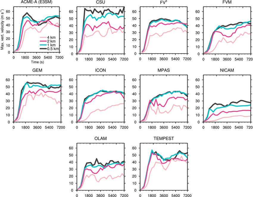
C. M. Zarzycki et al.: DCMIP2016: supercell 881
The definition of this test case relies on hydrostatic and cy- and iteration procedure
clostrophic wind balance, written in terms of Exner pressure
π and virtual potential temperature θv as Zz
(i) g
πeq = 1− (i)
dz (8)
cp θv,eq
∂π g ∂π 0
=− , and u2 tan ϕ = −cp θv . (1) cp /Rd
∂z cp θv ∂ϕ
(i) (i)
peq = p0 πeq (9)
Defining u = ueq cos ϕ to maintain solid body rotation, where (i)
Teq (i)
= θeq (z)πeq (10)
ueq is the equatorial wind velocity, these equations can be
combined to eliminate π , leading to (i)
(i) (i)
qeq = H (z)qvs peq , Teq (11)
2
!
∂θv sin(2ϕ) 2 ∂θv ∂ueq (i+1)
(i)
= ueq − θv . (2) θv,eq = θeq (z) 1 + Mv qeq . (12)
∂ϕ 2g ∂z ∂z
This iteration procedure generally converges to machine
The wind velocity is analytically defined throughout the epsilon after approximately 10 iterations. The equatorial
domain. Meridional and vertical wind is initially set to zero. moisture profile is then extended through the entire domain:
The zonal wind is obtained from
q(z, ϕ) = qeq (z). (13)
u(ϕ, z) = (3) Once the equatorial profile has been constructed, the vir-
tual potential temperature through the remainder of the do-
z
for z < zs − 1zu , main can be computed by iterating on Eq. (2):
Us − Uc cos(ϕ)
zs
θv(i+1) (z, ϕ) =
(14)
" ! #
4 z 5 z2 .
− +3 − Us − Uc cos(ϕ) for |z − zs | ≤ 1zu Zϕ !
zs 4 zs2 (i) ∂u2eq
5 sin(2φ) 2 ∂θv
(i)
θv,eq (z) + ueq − θv dϕ.
(Us − Uc ) cos(ϕ) for z > zs + 1zu 2g ∂z ∂z
0
The equatorial profile is determined through numerical it-
Again, approximately 10 iterations are needed for conver-
eration. Potential temperature at the Equator is specified via
gence to machine epsilon. Once virtual potential temperature
has been computed throughout the domain, Exner pressure
5
z 4 throughout the domain can be obtained from Eq. (1):
θ0 + (θtr − θ0 )
for 0 ≤ z ≤ ztr ,
θeq (z) = ztr , (4)
g(z − z ) Zϕ
θtr exp
tr
for ztr ≤ z u2 tan ϕ
cp Ttr π(z, ϕ) = πeq (z) − dϕ, (15)
cp θv
0
and relative humidity is given by and so
p(z, ϕ) = p0 π(z, ϕ)cp /Rd ,
3 z 5/4 (16)
1− for 0 ≤ z ≤ ztr ,
4 ztr Rd /cp
H (z) = (5) Tv (z, ϕ) = θv (z, ϕ)(p/p0 ) . (17)
1
for ztr ≤ z.
4 Note that, for Eqs. (13)–(14), Smolarkiewicz et al. (2017)
also derived an analytic solution for the meridional variation
It is assumed that the saturation mixing ratio is given by of the initial background state for shallow atmospheres.
380.0 T − 273.0
qvs (p, T ) = exp 17.27 × . (6)
p T − 36.0
Pressure and temperature at the Equator are obtained by
iterating on hydrostatic balance with initial state
(0)
θv,eq (z) = θeq (z), (7)
www.geosci-model-dev.net/12/879/2019/ Geosci. Model Dev., 12, 879–892, 2019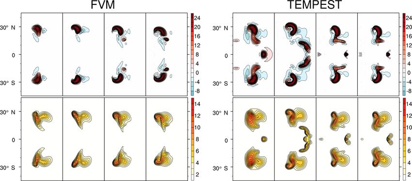
882                                                                                             C. M. Zarzycki et al.: DCMIP2016: supercell

Table 2. Participating modeling centers and associated dynamical cores that submitted results for the splitting supercell test.

      Short name              Long name                                                      Modeling center or group
      ACME-A (E3SM)           Energy Exascale Earth System Model                             Sandia National Laboratories and
                                                                                             University of Colorado, Boulder, USA
      CSU                     Colorado State University Model                                Colorado State University, USA
      FV3                     GFDL Finite-Volume Cubed-Sphere Dynamical Core                 Geophysical Fluid Dynamics Laboratory, USA
      FVM                     Finite Volume Module of the Integrated Forecasting System      European Centre for Medium-Range Weather Forecasts
      GEM                     Global Environmental Multiscale model                          Environment and Climate Change Canada
      ICON                    ICOsahedral Non-hydrostatic model                              Max-Planck-Institut für Meteorologie/DWD, Germany
      MPAS                    Model for Prediction Across Scales                             National Center for Atmospheric Research, USA
      NICAM                   Non-hydrostatic Icosahedral Atmospheric Model                  AORI/JAMSTEC/AICS, Japan
      OLAM                    Ocean Land Atmosphere Model                                    Duke University/University of Miami, USA
      TEMPEST                 Tempest Non-hydrostatic Atmospheric Model                      University of California, Davis, USA

2.2       Potential temperature perturbation                                       2.3   Physical and numerical diffusion

To initiate convection, a thermal perturbation is introduced                       As noted in Klemp et al. (2015), dissipation is an important
into the initial potential temperature field:                                      process near the grid scale, particularly in simulations inves-
                                                                                   tigating convection in unstable environments such as this. To
θ 0 (λ, φ, z) =                                                             (18)   represent this process and facilitate solution convergence as
                                                                                   resolution is increased for a given model, a second-order dif-
               π
                                                                                   fusion operator with a constant viscosity (value) is applied to
(
      1θcos2          Rθ (λ, ϕ, z)       for Rθ (λ, ϕ, z) < 1,
                  2                                                                all momentum equations (ν = 500 m2 s−1 ) and scalar equa-
      0                                  for Rθ (λ, ϕ, z) ≥ 1,                     tions (ν = 1500 m2 s−1 ). In the vertical, this diffusion is ap-
                                                                                   plied to the perturbation from the background state only in
where                                                                              order to prevent the initial perturbation from mixing out.
                   "                         2             2 #1/2                 Models that contributed supercell test results during
                        Rc (λ, ϕ; λp , ϕp )          z − zc                        DCMIP2016 are listed in Table 2. They are formally de-
Rθ (λ, ϕ, z) =                                     +                    .
                               rp                      zp                          scribed in Ullrich et al. (2017) and the references therein.
                                                                                   Further, specific versions of the code used in DCMIP2016
                                                                            (19)
                                                                                   and access instructions are also listed in Ullrich et al. (2017).
                                                                                   Note that not all DCMIP2016 participating groups submitted
   An additional iterative step is then required to bring the                      results for this particular test.
potential temperature perturbation into hydrostatic balance.                          Due to the multitude of differing implicit and explicit
Without this additional iteration, large vertical velocities will                  diffusion in the participating models, some groups chose
be generated as the flow rapidly adjusts to hydrostatic bal-                       to apply variations in how either horizontal or vertical dif-
ance since the test does not possess strong non-hydrostatic                        fusion were treated in this test case. Deviations from the
characteristics at initialization. Plots showing the initial state                 above-specified diffusion are as follows. CSU applied uni-
of the supercell are shown in Figs. 1 and 2 for reference.                         form three-dimensional second-order diffusion with coeffi-
Code used by modeling centers during DCMIP2016 for ini-                            cients of ν = 1500 m2 s−1 for qv and θv , ν = 1000 m2 s−1
tialization of the supercell test case is archived via Zen-                        for qc and qr , and ν = 500 m2 s−1 for divergence and rela-
odo (https://doi.org/10.5281/zenodo.1298671, Ullrich et al.,                       tive vorticity. FV3 applied divergence and vorticity damping
2018).                                                                             separately to the velocity fields along the floating Lagrangian
   The test case is designed such that the thermal perturbation                    surface. A Smagorinsky diffusion is also applied to the hori-
will induce a convective updraft immediately after initializa-                     zontal wind. ICON applied constant horizontal second-order
tion. As rainwater is generated by the microphysics, reduced                       diffusion to the horizontal and vertical velocity components
buoyancy and a subsequent downdraft at the Equator in com-                         (ν = 500 m2 s−1 ) as well as the scalar variables θv and qv,c,r
bination with favorable vertical pressure gradients near the                       (ν = 1500 m2 s−1 ). No explicit diffusion was applied in the
peripheral flanks of the storm will cause it to split into two                     vertical. NICAM applied a dynamically defined fourth-order
counter-rotating cells that propagate transversely away from                       diffusion to all variables in the horizontal with vertical dissi-
the Equator until the end of the test (Rotunno and Klemp,                          pation being implicitly handled by the model’s vertical dis-
1982, 1985; Rotunno, 1993; Klemp et al., 2015).                                    cretization.

Geosci. Model Dev., 12, 879–892, 2019                                                                  www.geosci-model-dev.net/12/879/2019/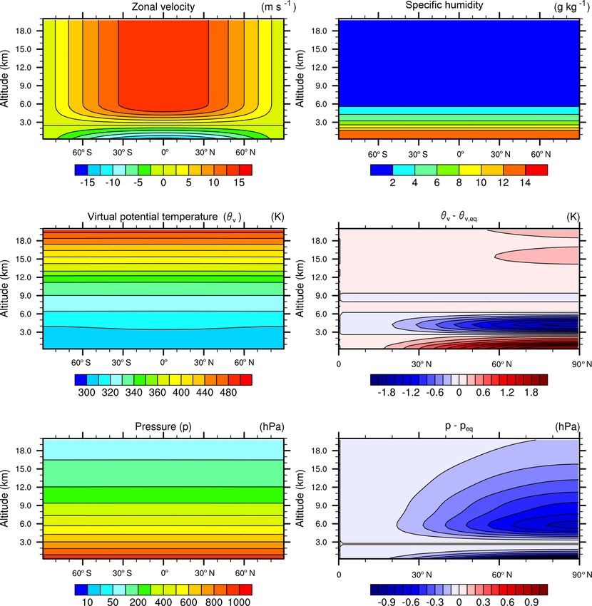
C. M. Zarzycki et al.: DCMIP2016: supercell 883
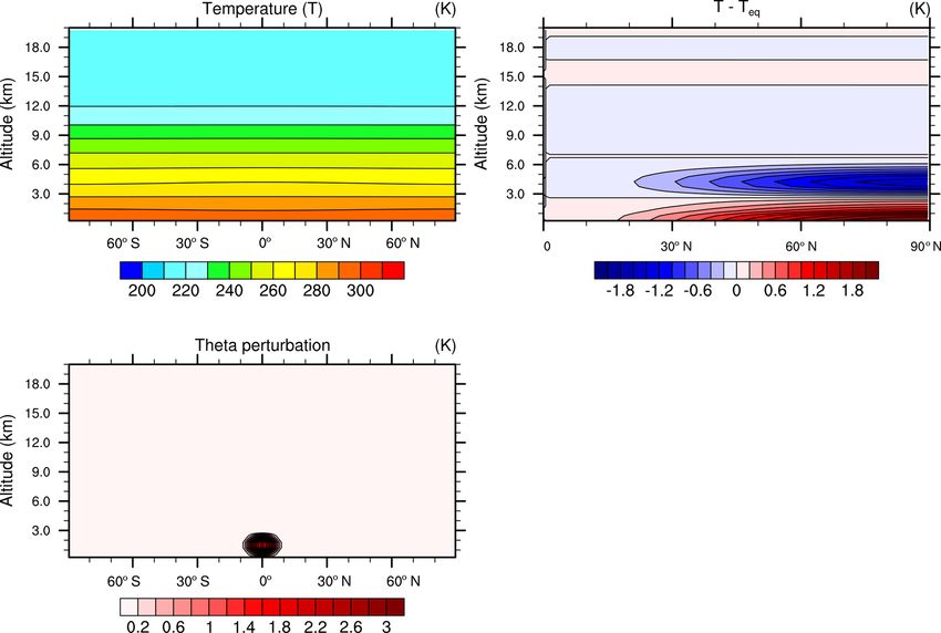
Figure 1. Initial state for the supercell test. All plots are latitude–height slices at 0◦ longitude. Deviations from equatorial values are shown
for virtual potential temperature and pressure.
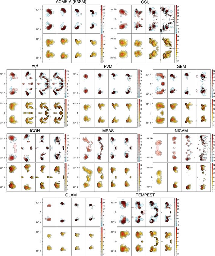
3 Results 3.1 Time evolution of supercell at control resolution
The following section describes the results of the supercell
Figure 3 shows the temporal evolution (every 30 min, out
test case during DCMIP2016, both from a intermodel time
to 120 min test termination) of the supercell for contributing
evolution perspective and intramodel sensitivity to model
models at the control resolution of 1 km. The top four pan-
resolution and ensuing convergence. Note that there is no an-
els for each model highlight a cross-section at 5 km elevation
alytic solution for the test case, but features specific to super-
through vertical velocity (w), while the bottom four show a
cells should be observed and are subsequently discussed. It
cross-section (at the same elevation) through the rainwater
is not the intent of this paper to formally explore the precise
(qr ) field produced by the Kessler microphysics. For w, red
mechanisms for model spread or define particular solutions
contours represent rising motion, while blue contours denote
as superior but rather to publish an overview set of results
sinking air. Note that the longitudes plotted vary slightly in
from a diverse group of global, non-hydrostatic models to be
each of the four time panes to account for zonal movement.
used for future development endeavors. Future work employ-
This analysis framework closely follows that originally out-
ing this test case in a more narrow sense can isolate some of
lined in Klemp et al. (2015).
the model design choices that impact supercell simulations.
All model solutions show bulk similarities. With respect
to vertical velocity, a single, horseshoe-shaped updraft is
www.geosci-model-dev.net/12/879/2019/ Geosci. Model Dev., 12, 879–892, 2019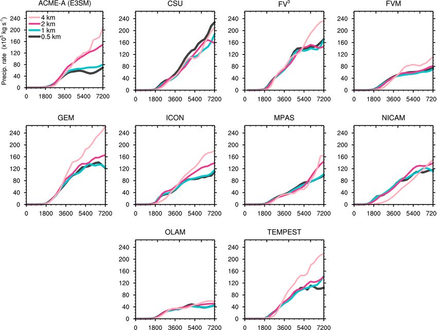
884 C. M. Zarzycki et al.: DCMIP2016: supercell
Figure 2. Same as Fig. 1 for temperature and potential temperature.
noted at 30 min in all models, although the degree to which MPAS all show two discrete supercells approximately 30◦
the maximum updraft velocities are centered on the Equator from the Equator. FV3 and TEMPEST both produce longi-
vary. A corresponding downdraft is located immediately to tudinally transverse storms that stretch towards the Equator
the east of the region of maximum positive vertical velocity. in addition to the two main cells. Each of the splitting super-
This downdraft is single-lobed (e.g., ACME-A) or double- cells splits a second time in ICON, forming, in conjunction
lobed (e.g., GEM) in all simulations. Separation of the initial with a local maximum at the Equator, five maxima of vertical
updraft occurs by 60 min across all models, although vari- velocity (and correspondingly rainwater). NICAM produces
ance begins to develop in the meridional deviation from the two core supercells (as more clearly evident in the qr field
Equator of the splitting supercell. Models such as NICAM, at 120 min) but has noticeable alternating weak updrafts and
FV3 , OLAM, and ICON all have larger and more distinct downdrafts in the north–south space between the two storm
north–south spatial separation, while FVM, GEM, ACME-A, cores.
and TEMPEST show only a few degrees of latitude between The relative smoothness of the storms as measured by
updraft cores. the vertical velocity and rainwater fields also varies between
Structural differences also begin to emerge at 60 min. For models, particularly at later times. ACME-A, FVM, GEM,
example, FVM, GEM, ACME-A, and TEMPEST all exhibit OLAM, and MPAS produce updrafts that are relatively free
three local maxima in vertical velocity: two large updrafts of additional, small-scale local extrema in the vicinity of the
mirrored about the Equator with one small maximum still core of the splitting supercell. Conversely, CSU, FV3 , ICON,
located over Equator centered near the initial perturbation. NICAM, and TEMPEST all exhibit solutions with additional
Similar behavior is noted in the qr fields. This is in contrast convective structures, with multiple updraft maxima versus
with other models which lack a third updraft on the equatorial two coherent cells. This spread is somewhat minimized when
plane. Generally speaking, qr maxima are collocated with the looking at rainwater, implying that the overall dynamical
locations of maximum updraft velocities and thereby conver- character of the cells as noted by precipitation generation
sion from qv and qc to qr in the Kessler microphysics. is more similar, with all models showing cohesive rainwater
While the aggregate response of a single updraft eventu- maxima O(10 g kg−1 ).
ally splitting into poleward-propagating symmetric storms
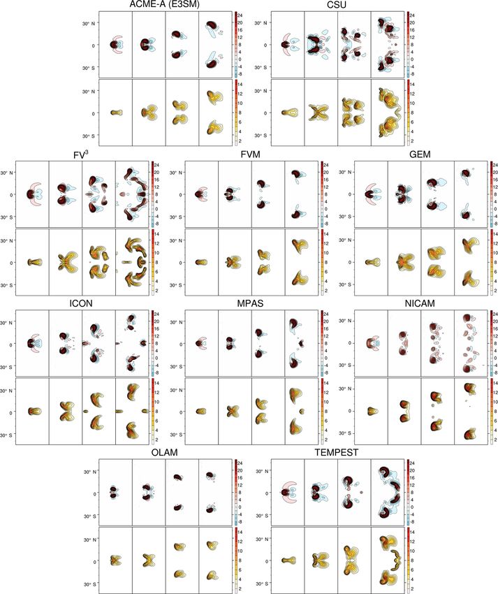
about the Equator is well matched between the configura- 3.2 Resolution sensitivity of the supercell
tions, notable differences exist, particularly towards the end
of the runs. At 120 min, FVM, GEM, ACME-A, OLAM, and Figure 4 shows the same cross-section variables as Fig. 3
except across the four specified test resolutions (nominally
Geosci. Model Dev., 12, 879–892, 2019 www.geosci-model-dev.net/12/879/2019/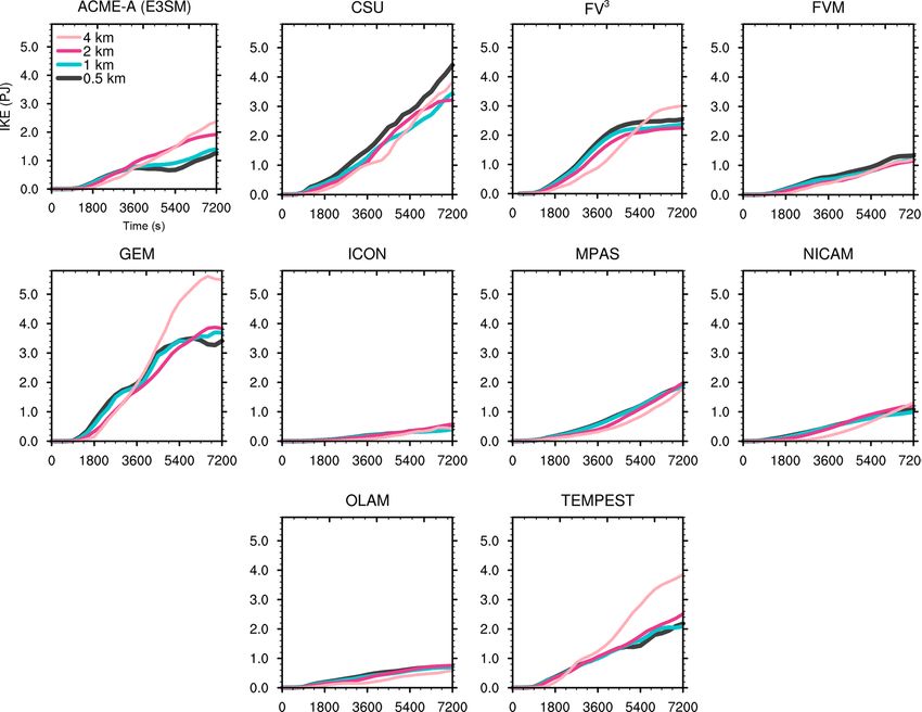
C. M. Zarzycki et al.: DCMIP2016: supercell                                                                                           885

Figure 3. Time evolution of cross-sections of 5 km vertical velocity (m s−1 , top) and 5 km rainwater (g kg−1 , bottom) for each model with
the r100 configuration of the test case. From left to right, fields are plotted at 30, 60, 90, and 120 min.

www.geosci-model-dev.net/12/879/2019/                                                         Geosci. Model Dev., 12, 879–892, 2019
886                                                                                  C. M. Zarzycki et al.: DCMIP2016: supercell

Figure 4. Resolution sensitivity of cross-sections of 5 km vertical velocity (m s−1 , top) and 5 km rainwater (g kg−1 , bottom) plotted at
120 min for each model. From left to right, nominal model resolutions are 4, 2, 1, and 0.5 km.

Geosci. Model Dev., 12, 879–892, 2019                                                      www.geosci-model-dev.net/12/879/2019/
C. M. Zarzycki et al.: DCMIP2016: supercell                                                                                         887

Figure 5. Maximum domain updraft velocity (m s−1 ) as a function of time (seconds from initialization) for each model at each of the four
specified resolutions. Note that the dark grey line is the finest grid spacing (0.5 km) in this test.

4, 2, 1, and 0.5 km, from left to right) at test termination           sult is likely due to the differences in explicit diffusion treat-
of 120 min. Therefore, the third panel from the left for each          ment as noted before, as well as differences in the numerical
model (1 km) should match the fourth panel from the left for           schemes’ implicit diffusion, particularly given the large im-
each model in Fig. 3.                                                  pact of dissipation on kinetic energy near the grid scale (Ska-
   As resolution increases (left to right), models show in-            marock, 2004; Jablonowski and Williamson, 2011; Guimond
creasing horizontal structure in both the vertical velocity            et al., 2016; Kühnlein et al., 2019). Additional focused sensi-
and rainwater fields. Updraft velocity generally increases             tivity runs varying explicit diffusion operators and magnitude
with resolution, particularly going from 4 to 2 km, implying           may be insightful for developers to explore. It is also hypoth-
that the supercell is underresolved at 4 km resolution. This           esized that differences in the coupling between the dynam-
is supported by previous mesoscale simulations investigat-             ical core and subgrid parameterizations may lead to some
ing supercells in other frameworks (Potvin and Flora, 2015;            of these behaviors (e.g., Staniforth et al., 2002; Gallus and
Schwartz et al., 2017), although it should be emphasized that          Bresch, 2006; Malardel, 2010; Thatcher and Jablonowski,
this response is also subject to each numerical scheme’s ef-           2016; Gross et al., 2018), although more constrained sim-
fective resolution (Skamarock, 2004) and that the resolvabil-          ulations isolating physics–dynamics coupling in particular
ity of real-world supercells can depend on the size of indi-           modeling frameworks is a target for future work. As before,
vidual storms.                                                         rainwater cross-sections tend to be less spatially variable at
   At the highest resolutions, there is a distinct group of mod-       0.5 km than vertical velocity, although CSU and NICAM
els that exhibit more small-scale structure, particularly in ver-      both show some additional local maxima in the field asso-
tical velocity, at +120 min at higher resolutions. CSU, GEM,           ciated with some of the aforementioned w maxima.
and NICAM appear to have the largest vertical velocity vari-
ability at 0.5 km, while ACME-A, FVM, MPAS, and TEM-
PEST appear to produce the smoothest solutions. This re-

www.geosci-model-dev.net/12/879/2019/                                                        Geosci. Model Dev., 12, 879–892, 2019
888                                                                                   C. M. Zarzycki et al.: DCMIP2016: supercell

Figure 6. Same as Fig. 5 except showing area-integrated instantaneous precipitation rate (×105 kg s−1 ).

3.3   Convergence of global supercell quantities with                   are necessary to achieve convergence; this is left to the indi-
      resolution                                                        vidual modeling groups to verify (see Sect. 3.4 for an exam-
                                                                        ple).
While Fig. 4 highlights the structural convergence with res-               The maximum updraft velocity as a function of resolu-
olution, more storm-wide measures of supercell intensity are            tion for particular model configurations varies quite widely.
also of interest. Figure 5 shows the maximum resolved up-               NICAM produces the weakest supercell, with velocities
draft velocity over the global domain as a function of time             around 30 m s−1 at 0.5 km, while ACME-A, TEMPEST,
for each dynamical core and each resolution (finer model                GEM, and CSU all produce supercells that surpass 55 m s−1
resolution is denoted by progressively darker lines). Maxi-             at some point during the supercell evolution. Models that
mum updraft velocity is chosen as a metric of interest due to           have weaker supercells at 0.5 km tend to also have weaker
its common use in both observational and modeling studies               supercells at 4 km (e.g., NICAM), while the same is true for
of supercells. All models show increasing updraft velocity              stronger supercells (e.g., TEMPEST), likely due to config-
as a function of resolution, further confirming that, at 4 km,          uration sensitivity. This agrees with the already discussed
the supercell is underresolved dynamically. For the major-              structural plots (Fig. 4) which demonstrated model solutions
ity of models and integration times, the gap between 4 and              were generally converging with resolution on an intramodel
2 km grid spacing is the largest in magnitude, with subse-              basis but not necessarily across models.
quent increases in updraft velocity being smaller as models                Figure 6 shows the same analysis except for area-
further decrease horizontal grid spacing. At 0.5 km, the ma-            integrated precipitation rate for each model and each reso-
jority of models are relatively converged, with FV3 , ICON,             lution. Similar results are noted as above – with most mod-
and MPAS showing curves nearly on top of one another at                 els showing large spread at the coarsest resolutions but gen-
these resolutions. Other models show larger differences be-             eral convergence in precipitation by 0.5 km. All models pro-
tween 0.5 and 1 km curves, implying that these configura-               duce the most precipitation at 120 min with the 4 km sim-
tions may not yet be converged in this bulk sense. Further              ulation. This is consistent with Klemp et al. (2015), who
grid refinement or modifications to the dissipation schemes             postulated this behavior is due to increased spatial extent of

Geosci. Model Dev., 12, 879–892, 2019                                                        www.geosci-model-dev.net/12/879/2019/
C. M. Zarzycki et al.: DCMIP2016: supercell 889 Figure 7. Same as Fig. 5 except showing storm-integrated kinetic energy (PJ) as defined in Eq. (20). Figure 8. As in Fig. 4 except showing the subset of models that completed a 0.25 km test. From left to right, nominal model resolutions are 2, 1, 0.5, and 0.25 km. www.geosci-model-dev.net/12/879/2019/ Geosci. Model Dev., 12, 879–892, 2019
890 C. M. Zarzycki et al.: DCMIP2016: supercell
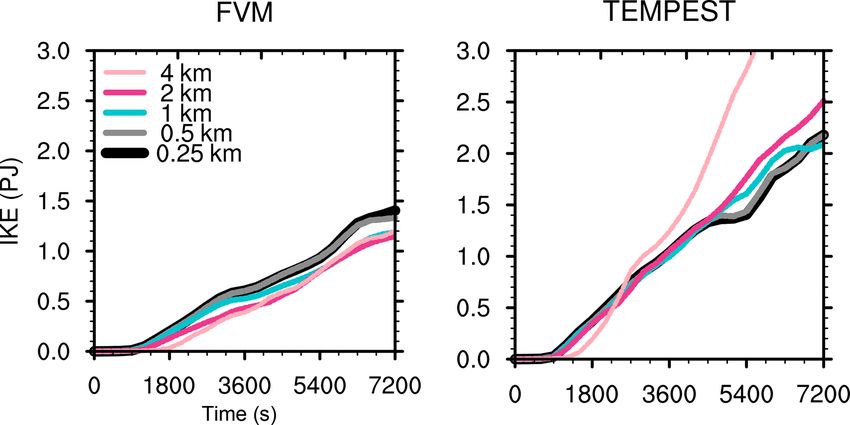
has not been reached for some of the modeling groups (e.g.,
Sect. 3.3). To confirm that the solution still converges further,
two groups (FVM and TEMPEST) completed an exploratory
set of simulations at 0.25 km resolution. Figure 8 shows the
structural grid spacing convergence at 120 min for the two
models from 2 to 0.25 km. Note that the left three panels for
each model in Fig. 8 should match the corresponding three
rightmost panels in Fig. 4. Figure 9 shows FVM and TEM-
PEST IKE results, including the 0.25 km simulations.
For TEMPEST and FVM, results indicate solution differ-
ences are markedly smaller between 0.5 and 0.25 km than be-
Figure 9. As in Fig. 7 except showing the subset of models that tween 1 and 0.5 km, implying the test is not fully converged
completed a 0.25 km test. at 0.5 km for these models. Therefore, 0.25 km may be a bet-
ter target for a reference grid spacing going forward.
It is worth noting that the reference solution in Klemp et al.
available qr to fall out of the column at these grid spacings,
(2015) is indeed converged at 0.5 km, as are some of the mod-
even though updraft velocities are weaker at coarser resolu-
els in DCMIP2016. Given this, it is unclear whether the need
tions. Unlike maximum vertical velocity, the integrated pre-
to go beyond DCMIP2016 protocols for “full” convergence
cipitation rate does not monotonically increase with resolu-
is due to the test case definition itself or, rather, the imple-
tion for most models. At 120 min, integrated rates at 0.5 km
mentation of the test case in particular models. This is left
range by approximately a factor of 3 or 4, from a low of 50–
for subsequent analyses. However, given this result, it is rec-
70 ×105 kg s−1 (ACME-A, FVM, OLAM) to a high of 170–
ommended that groups applying this test case in the future
200 ×105 kg s−1 (CSU, FV3 ), highlighting the sensitivity of
continue to push beyond the four resolutions specified here if
final results that have been already been discussed.
convergence is not readily apparent in either storm structure
In addition to Figs. 5 and 6, which directly correspond
or bulk quantities at 0.5 km.
to analysis in Klemp et al. (2015), we also define a storm-
integrated kinetic energy (IKE) metric as follows:
Zzt ZAe 4 Conclusions
1 2 2 2
IKE(t) = ρ u0 + v 0 + w0 dAdz, (20)
2 Non-hydrostatic dynamics are required for accurate repre-
0 0 sentation of supercells. The results from this test case show
where zt is the model top, Ae is the area of the sphere, and that clear differences and uncertainties exist in storm evolu-
winds (u0 , v 0 , w 0 ) are calculated as perturbations from the tion when comparing identically initialized dynamical cores
initial model state at the corresponding spatial location (e.g., at similar nominal grid resolutions. Intramodel convergence
u0 = u0 (t, φ, ψ, z) = u(t, φ, ψ, z)−u(0, φ, ψ, z)). Here, local in bulk, integrated quantities appears to generally occur at
air density, ρ(t, φ, ψ, z), is computed using a standard atmo- approximately 0.5 km grid spacing. However, intermodel dif-
sphere due to limitations in available data from some groups. ferences are quite large even at these resolutions. For exam-
As a metric, IKE is less sensitive to grid-scale velocities ple, maximum updraft velocity within a storm between two
and is also a more holistic measure of storm-integrated inten- models may vary by almost a factor of 2 even at the highest
sity. This is shown in Fig. 7. Results are generally analogous resolutions assessed at DCMIP2016.
to those in Fig. 6. This should be expected since total precip- Structural convergence is weaker than bulk-integrated
itation within a supercell is tied to the spatial extent and mag- metrics. Two-dimensional horizontal cross-sections through
nitude of the upward velocities that dominate the IKE term. the supercells at various times show that some models are
Convergence behavior between 1 and 0.5 km appears simi- well converged between 1 and 0.5 km, while results from
lar for each model as noted earlier. The total spread across other models imply that finer resolutions are needed to as-
models at the end of the simulation for the 0.5 km simula- sess whether convergence will occur with a particular test
tions is also similar to that seen in Fig. 6, demonstrating the case formulation and model configuration. Interestingly, in
large range in “converged” solutions across models due to some cases, maximum bulk quantities converge faster than
the various design choices discussed earlier. snapshots of cross-sections.
We postulate that these differences and uncertainties likely
3.4 Sample experiments at 0.25 km grid spacing stem from not only the numerical discretization and grid
differences outlined in Ullrich et al. (2017) but also from
While the formal supercell test case definition during the form and implementation of filtering mechanisms (ei-
DCMIP2016 specified 0.5 km grid spacing as the finest res- ther implicit or explicit) specific to each modeling center.
olution for groups to submit, it is clear that full convergence The simulation of supercells at these resolutions are particu-
Geosci. Model Dev., 12, 879–892, 2019 www.geosci-model-dev.net/12/879/2019/C. M. Zarzycki et al.: DCMIP2016: supercell 891
larly sensitive to numerical diffusion since damping of prog- Systems Laboratory, the Department of Energy Office of Science
nostic variables in global models is occurring at or near the (award no. DE-SC0016015), the National Science Foundation
scales required for resolvability of the storm. This is differ- (award no. 1629819), the National Aeronautics and Space Ad-
ent from other DCMIP2016 tests (baroclinic wave and trop- ministration (award no. NNX16AK51G), the National Oceanic
ical cyclone), which produced dynamics that were less non- and Atmospheric Administration Great Lakes Environmental
Research Laboratory (award no. NA12OAR4320071), the Office
hydrostatic in nature and required resolvable scales much
of Naval Research and CU Boulder Research Computing. This
coarser than the grid cell level. Further, since DCMIP2016 work was made possible with support from our student and
did not formally specify a particular physics–dynamics cou- postdoctoral participants: Sabina Abba Omar, Scott Bachman,
pling strategy, it would not be surprising for particular design Amanda Back, Tobias Bauer, Vinicius Capistrano, Spencer Clark,
choices regarding how the dynamical core is coupled to sub- Ross Dixon, Christopher Eldred, Robert Fajber, Jared Fer-
grid parameterizations to also impact results. guson, Emily Foshee, Ariane Frassoni, Alexander Goldstein,
Given the lack of an analytic solution, we emphasize that Jorge Guerra, Chasity Henson, Adam Herrington, Tsung-
the goal of this paper is not to define particular supercells Lin Hsieh, Dave Lee, Theodore Letcher, Weiwei Li, Laura Maz-
as optimal answers. Rather, the main intention of this test at zaro, Maximo Menchaca, Jonathan Meyer, Farshid Nazari,
DCMIP2016 was to produce a verifiable database for models John O’Brien, Bjarke Tobias Olsen, Hossein Parishani, Charles Pel-
to use as an initial comparison point when evaluating non- letier, Thomas Rackow, Kabir Rasouli, Cameron Rencurrel,
Koichi Sakaguchi, Gökhan Sever, James Shaw, Konrad Simon,
hydrostatic numerics in dynamical cores. Pushing grid spac-
Abhishekh Srivastava, Nicholas Szapiro, Kazushi Takemura,
ings to 0.25 km and beyond to formalize convergence would Pushp Raj Tiwari, Chii-Yun Tsai, Richard Urata, Karin van der
be a useful endeavor in future application of this test, either Wiel, Lei Wang, Eric Wolf, Zheng Wu, Haiyang Yu, Sungduk Yu,
at the modeling center level or as part of future iterations of and Jiawei Zhuang. We would also like to thank Rich Loft,
DCMIP. Variable-resolution or regionally refined dynamical Cecilia Banner, Kathryn Peczkowicz and Rory Kelly (NCAR),
cores may reduce the burden of such simulations, making Carmen Ho, Perla Dinger, and Gina Skyberg (UC Davis), and
them more palatable for researchers with limited computing Kristi Hansen (University of Michigan) for administrative support
resources. during the workshop and summer school. The National Center for
We acknowledge that, as groups continue to develop non- Atmospheric Research is sponsored by the National Science Foun-
hydrostatic modeling techniques, small changes in the treat- dation. Sandia National Laboratories is a multimission laboratory
ment of diffusion in the dynamical core will likely lead to managed and operated by National Technology and Engineering
Solutions of Sandia, LLC, a wholly owned subsidiary of Honeywell
changes in their results from DCMIP2016. We recommend
International Inc., for the US Department of Energy’s National
modeling centers developing or optimizing non-hydrostatic Nuclear Security Administration under contract DE-NA0003525.
dynamical cores to perform this test and compare their so-
lutions to the baselines contained in this paper as a check of Edited by: Simone Marras
sanity relative to a large and diverse group of next-generation Reviewed by: two anonymous referees
dynamical cores actively being developed within the atmo-
spheric modeling community.
Code availability. Information on the availability of source code References
for the models featured in this paper can be found in Ullrich
et al. (2017). For this particular test, the initialization routine, Browning, K. A.: Airflow and Precipitation Trajectories Within Se-
microphysics code, and sample plotting scripts are available at vere Local Storms Which Travel to the Right of the Winds,
https://doi.org/10.5281/zenodo.1298671 (Ullrich et al., 2018). J. Atmos. Sci., 21, 634–639, https://doi.org/10.1175/1520-
0469(1964)0212.0.CO;2, 1964.
Doswell, C. A. and Burgess, D. W.: Tornadoes and toraadic storms:
A review of conceptual models, The Tornado: Its Structure, Dy-
Author contributions. CMZ prepared the text and corresponding
namics, Prediction, and Hazards, Geophysical Monograph Se-
figures in this paper. PAU assisted with formatting of the test case
ries, American Geophysical Union, 161–172, 1993.
description in Sect. 2. Data and notations about model-specific con-
Gallus, W. A. and Bresch, J. F.: Comparison of Impacts of WRF
figurations were provided by all co-authors representing their mod-
Dynamic Core, Physics Package, and Initial Conditions on Warm
eling groups.
Season Rainfall Forecasts, Mon. Weather Rev., 134, 2632–2641,
https://doi.org/10.1175/MWR3198.1, 2006.
Gross, M., Wan, H., Rasch, P. J., Caldwell, P. M., Williamson,
Competing interests. The authors declare that they have no conflict D. L., Klocke, D., Jablonowski, C., Thatcher, D. R., Wood,
of interest. N., Cullen, M., Beare, B., Willett, M., Lemarié, F., Blayo,
E., Malardel, S., Termonia, P., Gassmann, A., Lauritzen, P.
H., Johansen, H., Zarzycki, C. M., Sakaguchi, K., and Le-
Acknowledgements. DCMIP2016 is sponsored by the National ung, R.: Physics–Dynamics Coupling in Weather, Climate, and
Center for Atmospheric Research Computational Information Earth System Models: Challenges and Recent Progress, Mon.
www.geosci-model-dev.net/12/879/2019/ Geosci. Model Dev., 12, 879–892, 2019892 C. M. Zarzycki et al.: DCMIP2016: supercell
Weather Rev., 146, 3505–3544, https://doi.org/10.1175/mwr-d- Rotunno, R. and Klemp, J.: On the Rotation and Prop-
17-0345.1, 2018. agation of Simulated Supercell Thunderstorms, J. At-
Guimond, S. R., Reisner, J. M., Marras, S., and Giraldo, mos. Sci., 42, 271–292, https://doi.org/10.1175/1520-
F. X.: The Impacts of Dry Dynamic Cores on Asymmet- 0469(1985)0422.0.CO;2, 1985.
ric Hurricane Intensification, J. Atmos. Sci., 73, 4661–4684, Rotunno, R. and Klemp, J. B.: The Influence of the Shear-
https://doi.org/10.1175/JAS-D-16-0055.1, 2016. Induced Pressure Gradient on Thunderstorm Motion, Mon.
Jablonowski, C. and Williamson, D. L.: The pros and cons of dif- Weather Rev., 110, 136–151, https://doi.org/10.1175/1520-
fusion, filters and fixers in atmospheric general circulation mod- 0493(1982)1102.0.CO;2, 1982.
els, in: Numerical Techniques for Global Atmospheric Models, Schwartz, C. S., Romine, G. S., Fossell, K. R., Sobash, R. A.,
Springer, 381–493, 2011. and Weisman, M. L.: Toward 1-km Ensemble Forecasts
Ji, M. and Toepfer, F.: Dynamical Core Evaluation Test Report for over Large Domains, Mon. Weather Rev., 145, 2943–2969,
NOAA’s Next Generation Global Prediction System (NGGPS), https://doi.org/10.1175/MWR-D-16-0410.1, 2017.
Tech. rep., National Oceanic and Atmospheric Administration, Skamarock, W. C.: Evaluating Mesoscale NWP Models Using
available at: https://repository.library.noaa.gov/view/noaa/18653 Kinetic Energy Spectra, Mon. Weather Rev., 132, 3019–3032,
(last access: 25 February 2019), 2016. https://doi.org/10.1175/MWR2830.1, 2004.
Kessler, E.: On the Distribution and Continuity of Water Substance Smolarkiewicz, P. K., Kühnlein, C., and Grabowski, W. W.:
in Atmospheric Circulations, American Meteorological Soci- A finite-volume module for cloud-resolving simulations of
ety, Boston, MA, 1–84, https://doi.org/10.1007/978-1-935704- global atmospheric flows, J. Comput. Phys., 341, 208–229,
36-2_1, 1969. https://doi.org/10.1016/j.jcp.2017.04.008, 2017.
Klemp, J. B. and Wilhelmson, R. B.: The simulation of three- Staniforth, A., Wood, N., and Côté, J.: Analysis of the numerics of
dimensional convective storm dynamics, J. Atmos. Sci., 35, physics–dynamics coupling, Q. J. Roy. Meteor. Soc., 128, 2779–
1070–1096, 1978. 2799, https://doi.org/10.1256/qj.02.25, 2002.
Klemp, J. B., Skamarock, W. C., and Park, S.-H.: Idealized Thatcher, D. R. and Jablonowski, C.: A moist aquaplanet variant
global nonhydrostatic atmospheric test cases on a reduced- of the Held–Suarez test for atmospheric model dynamical cores,
radius sphere, J. Adv. Model. Earth Sy., 7, 1155–1177, Geosci. Model Dev., 9, 1263–1292, https://doi.org/10.5194/gmd-
https://doi.org/10.1002/2015MS000435, 2015. 9-1263-2016, 2016.
Kuang, Z., Blossey, P. N., and Bretherton, C. S.: A new Ullrich, P. A., Jablonowski, C., Kent, J., Lauritzen, P. H., Nair, R.,
approach for 3D cloud-resolving simulations of large-scale Reed, K. A., Zarzycki, C. M., Hall, D. M., Dazlich, D., Heikes,
atmospheric circulation, Geophys. Res. Lett., 32, L02809, R., Konor, C., Randall, D., Dubos, T., Meurdesoif, Y., Chen, X.,
https://doi.org/10.1029/2004gl021024, 2005. Harris, L., Kühnlein, C., Lee, V., Qaddouri, A., Girard, C., Gior-
Kühnlein, C., Deconinck, W., Klein, R., Malardel, S., Piotrowski, getta, M., Reinert, D., Klemp, J., Park, S.-H., Skamarock, W.,
Z. P., Smolarkiewicz, P. K., Szmelter, J., and Wedi, N. P.: FVM Miura, H., Ohno, T., Yoshida, R., Walko, R., Reinecke, A., and
1.0: a nonhydrostatic finite-volume dynamical core for the IFS, Viner, K.: DCMIP2016: a review of non-hydrostatic dynamical
Geosci. Model Dev., 12, 651–676, https://doi.org/10.5194/gmd- core design and intercomparison of participating models, Geosci.
12-651-2019, 2019. Model Dev., 10, 4477–4509, https://doi.org/10.5194/gmd-10-
Lemon, L. R. and Doswell, C. A.: Severe Thunderstorm Evolution 4477-2017, 2017.
and Mesocyclone Structure as Related to Tornadogenesis, Mon. Ullrich, P., Lauritzen, P. H., Reed, K., Jablonowski, C., Zarzy-
Weather Rev., 107, 1184–1197, https://doi.org/10.1175/1520- cki, C., Kent, J., Nair, R., and Verlet-Banide, A.: Cli-
0493(1979)1072.0.CO;2, 1979. mateGlobalChange/DCMIP2016: v1.0 (Version v1.0), Zenodo,
Malardel, S.: Physics–dynamics coupling, in: Proceedings of https://doi.org/10.5281/zenodo.1298671 (last access: 25 Febru-
ECMWF Workshop on Non-hydrostatic Modelling, European ary 2019), 2018.
Centre for Medium-Range Weather Forecasts, vol. 6777, 2010. Wedi, N. P. and Smolarkiewicz, P. K.: A framework for testing
Potvin, C. K. and Flora, M. L.: Sensitivity of Idealized Su- global non-hydrostatic models, Q. J. Roy. Meteor. Soc., 135,
percell Simulations to Horizontal Grid Spacing: Implications 469–484, https://doi.org/10.1002/qj.377, 2009.
for Warn-on-Forecast, Mon. Weather Rev., 143, 2998–3024, Weisman, M. L. and Klemp, J. B.: The Dependence
https://doi.org/10.1175/MWR-D-14-00416.1, 2015. of Numerically Simulated Convective Storms on
Reed, K. A., Bacmeister, J. T., Rosenbloom, N. A., Wehner, M. F., Vertical Wind Shear and Buoyancy, Mon. Weather
Bates, S. C., Lauritzen, P. H., Truesdale, J. E., and Hannay, C.: Rev., 110, 504–520, https://doi.org/10.1175/1520-
Impact of the dynamical core on the direct simulation of tropical 0493(1982)1102.0.CO;2, 1982.
cyclones in a high-resolution global model, Geophys. Res. Lett., Zhao, M., Held, I. M., and Lin, S.-J.: Some Counterintuitive Depen-
42, 3603–3608, https://doi.org/10.1002/2015GL063974, 2015. dencies of Tropical Cyclone Frequency on Parameters in a GCM,
Rotunno, R.: Supercell thunderstorm modeling and theory, J. Atmos. Sci., 69, 2272–2283, https://doi.org/10.1175/JAS-D-
The tornado: Its structure, dynamics, prediction, and haz- 11-0238.1, 2012.
ards, in: Geophysical Monograph Series, edited by: Church,
C., Burgess, D., Doswell, C., and Davies-Jone R., 57–73,
https://doi.org/10.1029/GM079, 1993.
Geosci. Model Dev., 12, 879–892, 2019 www.geosci-model-dev.net/12/879/2019/You can also read