Absolute Baltic Sea Level Trends in the Satellite Altimetry Era: A Revisit - mediaTUM
←
→
Page content transcription
If your browser does not render page correctly, please read the page content below
ORIGINAL RESEARCH
                                                                                                                                                    published: 28 May 2021
                                                                                                                                           doi: 10.3389/fmars.2021.647607

                                             Absolute Baltic Sea Level Trends in
                                             the Satellite Altimetry Era: A Revisit
                                             Marcello Passaro 1*, Felix L. Müller 1 , Julius Oelsmann 1 , Laura Rautiainen 2 ,
                                             Denise Dettmering 1 , Michael G. Hart-Davis 1 , Adili Abulaitijiang 3 , Ole B. Andersen 3 ,
                                             Jacob L. Høyer 4 , Kristine S. Madsen 4 , Ida Margrethe Ringgaard 4 , Jani Särkkä 2 ,
                                             Rory Scarrott 5 , Christian Schwatke 1 , Florian Seitz 1 , Laura Tuomi 2 , Marco Restano 6 and
                                             Jérôme Benveniste 7
                                             1
                                              Deutsches Geodätisches Forschungsinstitut der Technischen Universität München, Munich, Germany, 2 Marine Research
                                             Unit, Finnish Meteorological Institute, Helsinki, Finland, 3 Technical University of Denmark, National Space Institute, Lyngby,
                                             Denmark, 4 Danish Meteorological Institute, Copenhagen, Denmark, 5 Department of Geography, MaREI Centre,
                                             Environmental Research Institute, University College Cork, Cork, Ireland, 6 SERCO/ESRIN, Frascati, Italy, 7 European Space
                                             Agency-ESRIN, Frascati, Italy

                                             The absolute sea level trend from May 1995 to May 2019 in the Baltic Sea is analyzed by
                                             means of a regional monthly gridded dataset based on a dedicated processing of satellite
                                             altimetry data. In addition, we evaluate the role of the North Atlantic Oscillation and the
                            Edited by:
                       Gilles Reverdin,
                                             wind patterns in shaping differences in sea level trend and variability at a sub-basin
      Centre National de la Recherche        scale. To compile the altimetry dataset, we use information collected in coastal areas
          Scientifique (CNRS), France        and from leads within sea-ice. The dataset is validated by comparison with tide gauges
                       Reviewed by:          and the available global gridded altimetry products. The agreement between trends
                         Léon Chafik,
       Stockholm University, Sweden          computed from satellite altimetry and tide gauges improves by 9%. The rise in sea level
             Hindumathi Palanisamy,          is statistically significant in the entire region of study and higher in winter than in summer.
    Meteorological Service Singapore,
                           Singapore
                                             A gradient of over 3 mm/yr in sea level rise is observed, with the north and east of the
                 *Correspondence:
                                             basin rising more than the south-west. Part of this gradient (about 1 mm/yr) is directly
                    Marcello Passaro         explained by a regression analysis of the wind contribution on the sea level time series. A
            marcello.passaro@tum.de          sub-basin analysis comparing the northernmost part (Bay of Bothnia) with the south-west
                                             reveals that the differences in winter sea level anomalies are related to different phases
                   Specialty section:
         This article was submitted to       of the North-Atlantic Oscillation (0.71 correlation coefficient). Sea level anomalies are
                   Ocean Observation,        higher in the Bay of Bothnia when winter wind forcing pushes waters through Ekman
               a section of the journal
          Frontiers in Marine Science
                                             transport from the south-west toward east and north. The study also demonstrates the
       Received: 30 December 2020
                                             maturity of enhanced satellite altimetry products to support local sea level studies in areas
           Accepted: 20 April 2021           characterized by complex coastlines or sea-ice coverage. The processing chain used in
           Published: 28 May 2021
                                             this study can be exported to other regions, in particular to test the applicability in regions
                               Citation:
                                             affected by larger ocean tides.
  Passaro M, Müller FL, Oelsmann J,
          Rautiainen L, Dettmering D,        Keywords: sea level, satellite altimetry, North Atlantic Oscillation (NAO index), Baltic Sea, coastal altimetry
      Hart-Davis MG, Abulaitijiang A,
Andersen OB, Høyer JL, Madsen KS,
 Ringgaard IM, Särkkä J, Scarrott R,
        Schwatke C, Seitz F, Tuomi L,
                                             1. INTRODUCTION
 Restano M and Benveniste J (2021)
  Absolute Baltic Sea Level Trends in
                                             Coastal societies are forced to constantly adapt to changes in sea level (SL). Global SL products such
  the Satellite Altimetry Era: A Revisit.    as those produced by the European Space Agency’s Sea Level Climate Change Initiative (SLCCI)
            Front. Mar. Sci. 8:647607.       (Legeais et al., 2018), the Integrated Multi-Mission Ocean Altimeter Data for Climate Research
    doi: 10.3389/fmars.2021.647607           (Beckley et al., 2017), and the Copernicus services (Von Schuckmann et al., 2016), are proving to

Frontiers in Marine Science | www.frontiersin.org                                    1                                                 May 2021 | Volume 8 | Article 647607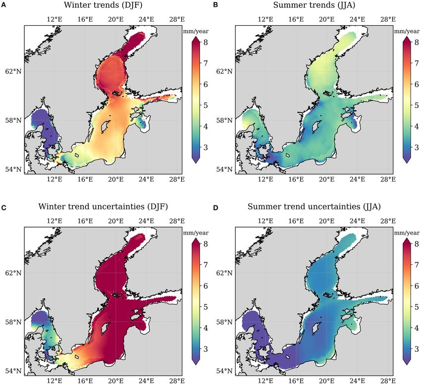
Passaro et al. Absolute Baltic Sea Level Trends
be instrumental in tracking the global SL rise, one of the most dataset and assessing its performances against in-situ data and
severe impacts of climate change. These synoptic and objective SL global gridded SL products. Subsequently, trends are computed
products are generated using the fleet of satellite-based altimeter providing statistical uncertainty that takes into account the serial
sensors in orbit for over two decades. However, for regional correlation in the time series.
to local coastal adaptation and planning for future scenarios,
regionally-tailored SL information is required.
In the Baltic Sea (BS), satellite observations are particularly
2. METHODS
important given that the network of tide gauge (TG)s, which 2.1. Altimetry Data Processing
measures relative SL, is strongly affected by Vertical Land Motion This study is based on the analysis of the ESA Baltic SEAL
(VLM) and, in particular, due to the Glacial Isostatic Adjustment project, whose documentation is freely available from http://
(GIA) (Ludwigsen et al., 2020). For example, relative SL trends in balticseal.eu/outputs/. In the context of this project, along-track
the northern part of the BS over the last few decades have been data from most of the altimetry missions operating in the last two
shown to be strongly negative, while absolute SL trends display decades are reprocessed to generate a dedicated monthly gridded
significant positive trends (Olivieri and Spada, 2016; Madsen product from May 1995 to May 2019. In particular the following
et al., 2019). While global altimetry products have been used to conventional Low Resolution Mode (LRM) altimetry missions
study SL in the area (Karabil et al., 2018), they are affected by data are used: TOPEX-Poseidon (TP, from May 1995), Jason-1 (J-
gaps that are smoothed out by the typical strong interpolation 1), Jason-2 (J-2), ERS-2, Envisat, and SARAL. Considering the
in space and time (Madsen et al., 2019). In particular, the BS latest Delay-Doppler (DD) altimetry technology, data from the
includes the two main features that limited the use of satellite following missions were acquired: Cryosat-2 (CS-2), Sentinel-3A,
altimetry since the start of the “altimetry era”: the presence of and Sentinel-3B (S3-A/B).
sea-ice and the proximity of the coast. For example, the average High-frequency data are downloaded, i.e., distributed at 20-
annual maximum extent of sea-ice in March covers up to 40% of Hz rate for most of the missions, except 10-Hz for TP, 40-Hz for
the water surface (Leppäranta and Myrberg, 2009), and there are SARAL, and 18-Hz for Envisat. A detailed list of the data source
around 200,000 islands in almost 400,000 km2 of water surface. and the version of the altimetry data acquired for the reprocessing
However, an advantage for using altimetry in the BS is that the is provided in Ringgaard et al. (2020).
tidal component is limited, which mitigates the known problems The overall process from radar pulse to SSH estimate delivered
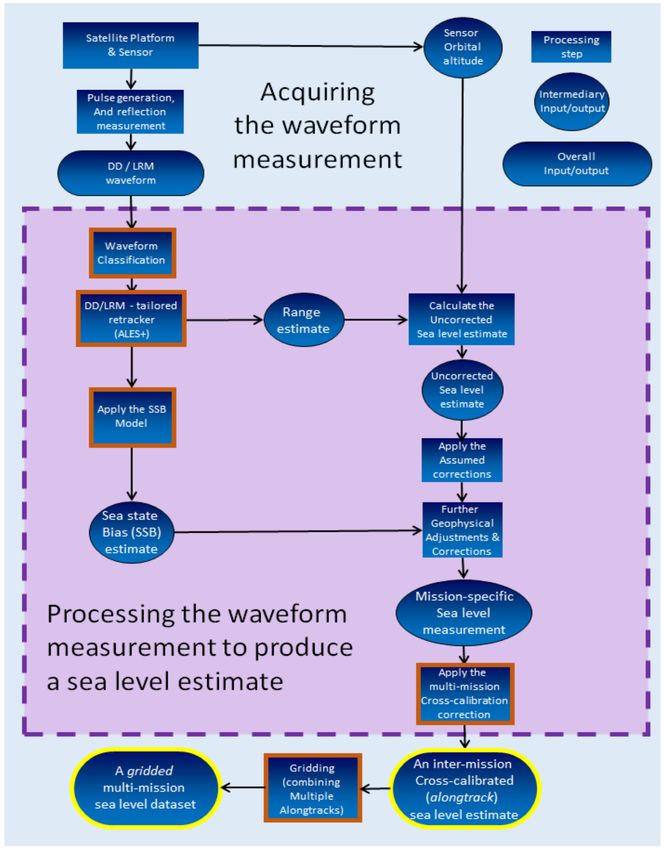
of tidal modelling in areas with complex coast and bathymetry. as a gridded product is outlined in Figure 1. Also outlined are the
The advances in altimetry processing have shown that enhancements which the ESA Baltic SEAL Project implements
dedicated signal processing techniques are able to enhance the to tailor the data produced to BS regional stakeholders, and
quality and the quantity of the retrievals (Benveniste et al., further develop best practice for coastal altimetry globally. These
2019). This is particularly significant when a better fitting of enhancements are summarised in the following sections and
the radar return (retracking) is combined with a dedicated build on the overall pulse-to-SL process.
selection of corrections to the altimetric range to enhance coastal
data (Benveniste et al., 2020). In the sea-ice covered areas, 2.1.1. Classification
classification techniques are able to identify water apertures In the winter months, parts of the BS, especially the regions Bay of
(leads), which when combined with retracking allow for the Bothnia and Gulf of Finland as defined in Figure 2, are covered
retrieval of SL. Such processing has recently driven an improved by a dynamic changing sea-ice cover, which makes continuous,
SL analysis in the Arctic Ocean (Rose et al., 2019), but has never gapless SL estimations difficult. Moreover, observations during
been applied to the BS yet. This gap presented an opportunity the winter season are limited to leads (i.e. narrow cracks within
for the European Space Agency’s Baltic+ Sea Level (ESA Baltic the sea-ice) enabling only brief, spatially limited opportunities for
SEAL) Project, to produce a regional gridded SL product open water measurements.
that incorporates observations from altimetry measurements The behaviour of the reflected radar signals is used to
acquired from sea-ice leads, and coastal waters. classify lead returns and to identify open water areas within
The use of dedicated altimetry SL products, combined the sea-ice. The applied open water detection is based on
with external datasets, can contribute to characterise local unsupervised, artificial intelligence machine-learning algorithms.
differences in SL trend and variability (Passaro et al., 2016). The algorithm used in this study has been described in Müller
The SL variability in the BS has been found to be highly et al. (2017) for LRM altimetry and its versatility to be applied
correlated with the variability of westerly winds (Andersson, also to DD missions has been shown in Dettmering et al. (2018).
2002). Wind patterns are modulated by large scale variability In order to group the reference datasets automatically into
of the atmospheric pressure, which can be described by climate a specific number of clusters representing different waveforms
indices, and in particular by the North Atlantic Oscillation types, the waveforms samples from a training set are introduced
(NAO) index (Jevrejeva et al., 2005). The objective of this to a K-medoids clustering algorithm (Xu and Wunsch, 2008;
study, therefore, is to analyse the SL trend in the BS during Celebi, 2014). In principle K-medoids searches for hidden
the altimetry era and to characterise the relationship between similarities within the data based on a given input feature space
wind patterns, NAO and variability in absolute SL at a sub- by minimizing the distance between the individual features and
basin scale. To do so, we use the ESA Baltic SEAL monthly most centrally positioned features (medoids) from the feature
gridded SL, summarising the methodology followed to create this space itself. At first the algorithm defines randomly K-medoids
Frontiers in Marine Science | www.frontiersin.org 2 May 2021 | Volume 8 | Article 647607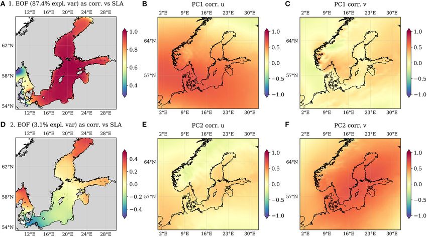
Passaro et al.                                                                                                                         Absolute Baltic Sea Level Trends

 FIGURE 1 | From measurement to corrected sea level estimates delivered as along-track and gridded datasets. A simple flowchart of the origins of the waveform data,
 and how it is processed to produce the ESA Baltic SEAL estimate of sea level. Process steps which are enhanced and tailored for use in BS, are highlighted in orange.

Frontiers in Marine Science | www.frontiersin.org                                 3                                               May 2021 | Volume 8 | Article 647607
Passaro et al.                                                                                                            Absolute Baltic Sea Level Trends

                                                                                  is based on the Brown-Hayne functional form that models the
                                                                                  radar returns from the ocean to the satellite. The Brown-Hayne
                                                                                  theoretical ocean model is the standard model for the open ocean
                                                                                  retrackers and describes the average return power of a rough
                                                                                  scattering surface (i.e., what we simply call waveform) (Brown,
                                                                                  1977; Hayne, 1980). A full description of ALES+ retracker for
                                                                                  LRM missions is provided in Passaro et al. (2018a).
                                                                                      In the case of the DD waveforms, the correspondent version
                                                                                  called ALES+ SAR adopts a simplified version of the Brown-
                                                                                  Hayne functional form as an empirical retracker to track the
                                                                                  leading edge of the waveform. The model simplification is
                                                                                  achieved by assigning a fixed decay of the trailing edge, instead of
                                                                                  a dependency with respect to antenna parameters (beamwidth,
                                                                                  mispointing) as in the LRM case. A full description of ALES+
                                                                                  SAR retracker is provided in Passaro et al. (2020a). Data from
                                                                                  CS-2, S3-A/B can be reprocessed with ALES+ SAR using the ESA
                                                                                  Grid Processing On Demand (GPOD) service (https://gpod.eo.
 FIGURE 2 | The area of study divided in different boxes representing major       esa.int/, Passaro et al., 2020b).
 sub-basins. Color shades display the bathymetry.                                     By means of a leading edge detection, ALES+ and ALES+ SAR
                                                                                  retrack only a subwaveform whose width is dependent on the
                                                                                  wave height in LRM and fixed in DD. In this way, it is possible to
                                                                                  avoid considering signal perturbations typical of the coastal zone
followed by the computation of the distance between all features                  when fitting the echoes. In the case of peaky waveforms, typical of
and the initially selected K centres. In the next steps K-medoids                 leads within sea-ice, both algorithms perform a direct estimation
rearranges the location of the medoids as long as there is                        of the trailing edge slope.
no motion among the features. K-medoids belongs to the                                Together with the retracking, a dedicated sea state bias (SSB)
“partitional” clustering algorithms, which require a pre-defined                  correction is computed. The SSB correction is computed at 20-
number of clusters K.                                                             Hz rate. This guarantees a better precision of the range retrieval,
    After clustering, the clusters are assigned manually to the                   since it decreases the impact of correlated errors in the retracked
different surface types, by using background knowledge about                      parameters (Passaro et al., 2018b).
the physical backscattering properties of the individual surface                      For the LRM missions, the SSB correction is derived by using
conditions and feature statistic per each cluster.                                the same 2D map from Tran et al. (2010), but computed for each
    The waveform features considered are the usual ones                           high-frequency point using the high-frequency wind speed and
describing the shape of the echo: waveform maximum, trailing                      significant wave height (SWH) estimations from ALES+.
edge decline (an exponential function fitted to the trailing edge of                  In the original DD altimetry products, the SSB correction is
the waveform), waveform noise, leading edge slope, trailing edge                  either missing (Cryosat-2) or computed using the Jason model.
slope. The features are applied to all required satellite missions                Here instead, a first model is computed specifically for the ALES+
and altimetry datasets.                                                           SAR retracker. As a reference parameter on which the model is
    The second part of the classification is related to the                       built, we take the rising time of the leading edge, which is taken
classification of the remaining waveforms. Therefore, a K-Nearest                 as a proxy for the significant wave height.
Neighbour (KNN) classifier is applied. KNN searches for the                           The corrections are derived by observing the SL residuals
closest distance between the reference model and the remaining                    (with no correction applied) at the points of intersections
waveforms (Hastie et al., 2009). The majority of clusters among                   between satellite tracks (crossover points). A wider region
the K nearest neighbours defines which class has to be assigned                   covering the North Sea and the Mediterranean Sea is used in
to the waveform.                                                                  order to have more open ocean crossover points, which are scarce
    As a final result of the classification, each high-frequency                  in the BS. The residuals are modelled with respect to the variables
waveform is classified as open water or sea-ice. Waveforms                        influencing the sea state (here the rising time of the leading edge)
classified as sea-ice returns are flagged and not considered for the              in a parametric formulation.
generation of the gridded product.                                                    In particular, at each crossover m:

2.1.2. Retracking                                                                                     1SLm = α̂σco − α̂σce + ǫ                        (1)
All the waveforms from the altimetry missions used in this study,
except for TP, are re-fitted by means of dedicated algorithms                     where o and e stand for odd and even tracks (indicating ascending
(retrackers) that are able to track the signal in open ocean, coastal,            and descending tracks respectively), ǫ accounts for residual
and sea-ice covered conditions.                                                   errors, σc is the rising time of the leading edge. We, therefore,
   ALES+ is the retracker that has been further developed and                     have a set of m linear equations, which is solved in a least square
extended to all the missions considered in this project. ALES+                    sense. The chosen α is the one that maximises the variance

Frontiers in Marine Science | www.frontiersin.org                             4                                       May 2021 | Volume 8 | Article 647607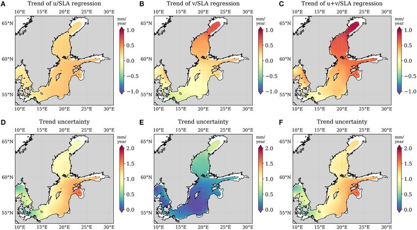
Passaro et al.                                                                                                                                Absolute Baltic Sea Level Trends

TABLE 1 | Altimeter corrections/parameter applied to the along-track processing.

Correction                                                                                              Missions

                                          TP              J-1a           J-2            J-3            ERS-2          Envisat        SARAL          CS-2             S3-A/B

Wet Trop.                                 GPD/GPD+                                      VFM3           GPD/GPD+                      VMF3 (Landskron and Böhm,
(WT)                                      (Fernandes et al., 2015;                      Landskron      (Fernandes et al.,            2018)
                                          Fernandes and Lazaro, 2016)                   and Böhm       2015; Fernandes and
                                                                                        (2018)         Lazaro, 2016)
Dry Trop.                                 ERA-Interim for Vienna Mapping Functions (VMF3) (Landskron and Böhm, 2018)
(DT)
Ionosphere                                NOAA Ionosphere Climatology (NIC09) (Scharroo and Smith, 2010)
(IONO)
Dynamic                                   DAC (inverse barometric (ECMWF), (MOG2D)HF) (Collecte Localisation Satellites , CLS)
Atmosphere
Corr. (DAC)
Solid Earth                               IERS Conventions 2010 (Petit and Luzum, 2010)
Tide (SET)
Pole Tide                                 IERS Conventions 2010 (Petit and Luzum, 2010)
(PT)
Sea State                                 MGDR            ALES+ (Passaro et al., 2018a)
Bias (SSB)
@l Radial Orbit                           Multi-mission cross calibration (MMXO) Vers. 18 (Bosch et al., 2014)
Errors (ROC)

a No   GPD/GPD+ (Fernandes et al., 2015; Fernandes and Lazaro, 2016) is available for J-1 geodetic mission phase. Instead, VMF3 Landskron and Böhm (2018) is used.

explained at the crossovers, i.e., the difference between the                                  The approach was developed for global calibration and is
variance of the crossover difference before and after correcting                            adapted for regional applications within ESA Baltic SEAL. This
for the SSB using the computed model.                                                       comprises the following points of change in comparison to
                                                                                            (Bosch et al., 2014):
2.1.3. Choice of Range Corrections
Once the ranges have been obtained by retracking the waveforms,                             1. The maximum acceptable time difference for the crossover
the following altimeter equation is implemented to derive the sea                              computations is increased from 2 to 3 days, in order to ensure
surface height (SSH):                                                                          enough crossover differences in the BS region.
                                                                                            2. For the same reason, all crossover points are used, including
       SSH = Horbit − (R + WT + DT + IONO + SSB + DAC                                          coastal areas.
                  +SET + PT + ROC)                                                (2)       3. For the computation of crossover differences, high frequency
                                                                                               data are used. This is realised by changing the interpolation of
The atmospheric and geophysical corrections applied are listed                                 along-track heights to crossover locations from point-wise to
in Table 1. Horbit and R stands for the orbital height above the                               distance-wise.
TOPEX/POSEIDON ellipsoid and the retracked range between                                    4. All missions are equally weighted. The weighting between
the satellite and the sea surface. To generate the gridded product,                            crossover differences and consecutive differences is adapted in
the SSH is also corrected for ocean tide and load tide using the                               order to account for the smaller region.
FES2014 tidal model (Carrere et al., 2015).

2.1.4. Multi-Mission Cross-Calibration                                                      2.1.5. Gridding
In order to ensure a consistent combination of all different                                After the multi-mission cross-calibration, the along-track SL
altimetry missions available, a cross-calibration is necessary. We                          estimates undergo an outlier detection whose consecutive steps
follow the global multi-mission crossover analysis (MMXO)                                   are listed in Passaro et al. (2020a). After this flagging, the
approach described by Bosch et al. (2014) in order to produce                               observations are interpolated on an unstructured triangular grid
a harmonized dataset and a consistent vertical reference for all                            (i.e., geodesic polyhedron). The grid has a spatial resolution
altimetry missions.                                                                         of 6–7 km.
    For all crossover locations, a radial correction for the                                    The gridded monthly SL estimates are obtained by fitting
observations of both intersecting tracks is estimated by a least                            an inclined plane to each grid node by means of weighted
squares approach based on crossover differences without the                                 least square interpolation, considering SSH along-track
application of any analytic error model. These corrections are                              information within 100 km radius around the grid node centre.
later interpolated to all measurement points of all missions                                Distance-based Gaussian weights are defined in a diagonal
included in the analysis.                                                                   matrix W. The median absolute deviation of the along-track

Frontiers in Marine Science | www.frontiersin.org                                       5                                                May 2021 | Volume 8 | Article 647607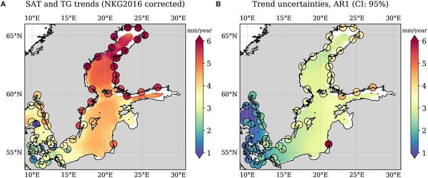
Passaro et al.                                                                                                       Absolute Baltic Sea Level Trends

SSH observation within an area in the open sea without complex             the latest GIA model for the BS. The closest absolute land uplift
topographic features is computed per mission and used as an                values are located for each TG and used for trend removal.
estimation of the uncertainty. This is placed as variance on the               The root mean square error (RMSE) and the Pearson
main diagonal of the uncertainty matrix Qbb . The uncertainty              correlation coefficient (r) are computed for all TG-grid pair time
information and W are combined to form the least-squares                   series and the results are displayed in Figure 3. Out of 67 TGs
weighting matrix Pbb , following the equation:                             and gridded altimetry pairs, 62 show a correlation higher than
                                                                           0.6 and 61 have a RMSE lower than 9 cm. The lowest performing
                                               1                           area is located north of the Danish straits. A possible reason lies
                              Pbb = W ∗ (         )             (3)
                                              Qbb                          in the performances of the tide corrections, which are much more
                                                                           important north of the straits, than in the BS.
In order to eliminate still existing outliers among the along-track            The results of the validation considering the sub-basin
data within the cap-size, the weighted least square estimation is          division used in this study are summarised in Table 2. For
performed iteratively. At each iteration, the difference between           this purpose, TG and altimetry gridded data are averaged in
the monthly average and all along-track SSH values is evaluated.           space across each sub-basin and in time every 3 months. The
The along-track estimates whose residual exceeds 3 times the               comparison shows that the correlation is never lower than 0.75
standard deviation of all residuals (3-sigma criterion) are flagged        and the RMSE is never higher than 0.10 m.
as outliers and the weighting matrix Pbb is consequently updated,
before a new least-squares adjustment is performed.                        2.3. Methods for SL Analysis
   Finally, an additional outlier rejection based on a Student             2.3.1. Trend Computation
distribution is performed: the standardised residuals of each              We estimate the seasonal cycle, the linear trend and the
remaining observations within the search radius are tested                 parameter uncertainties by fitting multi-year monthly averages
against quantiles of the Student distribution (t), setting the             (to approximate the seasonality) and a linear trend to the
99th percentile as boundary condition. If a standardised                   monthly gridded data. In terms of formulation, this means fitting
residual is smaller than the value of the t distribution, the              the time series d(t) with the model y(t), which for every monthly
corresponding observation is used in a last iteration of the least-        step t is defined as:
squares adjustment.
                                                                                                 y(t) = o + at + mi + ǫ                          (4)
2.2. Validation of the Altimetry Product
To validate the gridded SL product from altimetry, we perform              Where o is an offset term, a is the linear trend, mi is the multiyear
a comparison against SL data from TGs. The main source                     monthly mean for the month i corresponding to the time step
of data is the Copernicus Marine Environment Monitoring                    t and ǫ is the residual noise. The trend estimate is found solving
Service (CMEMS) service and some data are complemented                     the fitting by linear least squares. The standard error σ of the least
from the national datasets of the Danish Meteorological Institute          square solution would be nevertheless unrealistic, since it would
(DMI), the Finnish Meteorological Institute (FMI) and the                  not consider the autocorrelation of the time series. Therefore,
Swedish Meteorological and Hydrological Institute (SMHI). A                to account for the autocorrelation, σ is found by an iterative
full list of TG data sources used in this study is available in            maximum likelihood estimation (MLE), as described in [6]. This
Ringgaard et al. (2020).                                                   requires the definition of an appropriate covariance matrix of the
    To avoid gaps in the time series, we consider only grid points         observations, including a formulation of the residual noise. In
with at least 250 months of valid data. We also divide the BS in           particular, we investigate the fit of a variety of different stochastic
different sub-basins whose naming and geographical extensions              noise model combinations as done in e.g., Royston et al. (2018):
are provided in Figure 2.                                                  These are an autoregressive AR(1) noise model, a power law
    The TG and altimeter SL measurements are not equivalent                plus white, a generalized Gauss Markov (GGM) plus white,
and hence both data sets were further processed before they were           a Flicker noise plus white and an auto-regressive fractionally-
compared. In particular, to allow the comparison, the DAC was              integrated moving-average (ARFIMA) model. For the considered
added back to the altimetry data, since TG data is not corrected           domain we find that on average the AR(1) has the lowest mean
for it.                                                                    (or median) values of the Akaike Information Criterion (AIC,
    The SL reference frame of the altimeter SL height is tied to           Akaike, 1998) and the Bayesian Information Criterion (BIC,
the TOPEX ellipsoid, while TG SL height data are referred to the           Schwarz, 1978). Finally, the uncertainties provided in this study
Normaal Amsterdams Peil (NAP) reference frame. To allow for                are scaled as 1.96 ∗ σ to obtain a 95% confidence interval.
comparison of the TG-altimetry pairs, the mean of the gridded SL
was removed and set equal to the mean of the corresponding TG.             2.3.2. Principal Component Analysis
    In order to validate the gridded dataset, the grid points within       We perform a Principal Component Analysis (PCA)
20 km from every TG are considered. As the gridded dataset has             (Preisendorfer, 1988) to investigate the major modes of SL
a frequency of a month, the TG data are monthly averaged. TGs              variability in the BS. For this purpose, we consider a set
measure relative SL and altimeters measure absolute SL, hence              of multiple SL anomalies xk (t), where k and t describe the
the effect of land uplift is removed from the TG data using the            dimensionality of the data in space and time, respectively. To
GIA model NKG2016LU (Vestøl et al., 2019). NKG2016LU is                    identify the maximum modes of joint space and time variations,

Frontiers in Marine Science | www.frontiersin.org                      6                                         May 2021 | Volume 8 | Article 647607
Passaro et al.                                                                                                                      Absolute Baltic Sea Level Trends

 FIGURE 3 | Correlation coefficient and root mean square error between every TG considered and the altimetry grid points used for trend computation which are
 located within 20 km. The circles showing the statistics are co-located with the TGs.

TABLE 2 | Pearson Correlation Coefficient and RMSE between TGs and gridded               in this description, since it is the anomaly with respect to a
altimetry averaged in space over the sub-basins considered in this study and in          monthly-based average (for example, based on the average for
time every 3 months.
                                                                                         all Januaries in the period of record at a particular grid point).
Sub-basin                      r            RMSE (m)               Num of samples        In this way we capture the “full-year” monthly variability and no
                                                                                         seasonal variations. Because monthly SL variability is generally
Skagerrak+Kattegat           0.75              0.08                    1,698             most pronounced in winter, the derived full year EOF-pattern
S-W Baltic Sea               0.76              0.07                    3,367             are very similar to the ones derived only over the winter season
Gotland Basin                0.91              0.07                    1,336             (DJF). EOF patterns are given as point-wise correlations of their
Gulf of Riga                 0.92              0.08                     145              PCs with SLAs.
Gulf of Finland              0.91              0.08                    1,318
Sea of Bothnia               0.84              0.10                    1,612             2.3.3. Regression Analysis
Bay of Bothnia               0.88              0.09                     112              We use a simple statistical approach to understand the relation
                                                                                         of surface winds and SL trends: We compute point-wise
                                                                                         linear regressions of the deseasoned, monthly and basin-
                                                                                         averaged surface winds (zonal U component and meridional
we determine a set of linear combinations in form of Principal                           V component) and SLAs by solving for: SLA(t) = aU(t) +
Component (PC) um (t) and associated eigenvectors or Empirical                           bV(t) + η, where a and b are the first order partial regression
Orthogonal Function (EOF) ekm . The linear combinations,                                 coefficients to be estimated and η is the residual (e.g., Storch
or the modes are arranged such that the higher-order modes                               and Zwiers, 1999; Dangendorf et al., 2013). Based on these
m = 1, 2, 3, . . . explain the highest variance fractions of the data.                   point-wise linear regressions we estimate a linear trend (without
The PCs um (t) are equal to the projection of the data vector onto                       seasonal component) which is explained by the individual wind
the mth eigenvector ek m (e.g., Wilks, 2006):                                            components as well as the explained variance of SL variability by
                                                                                         the components (as for example in Dangendorf et al., 2013).
                             X
                             K
                  um (t) =          ekm xk (t), m = 1, . . . , M               (5)       3. RESULTS AND DISCUSSION
                             k=1
                                                                                         3.1. Absolute Sea Level Trends
In this manner the data is explained by a set of PCs, which                              Figure 4 shows the map of SL trends estimated using the ESA
represent time series (which are uncorrelated or independent                             Baltic SEAL dataset. Superimposed in circles along the coast are
from each other), as well as the EOFs (or eigenvectors) which                            the estimations of the TGs, which are corrected for GIA. In
represent the geographical coherence of the individual modes.                            accordance to previous studies based on the altimetry era (e.g.,
   We compute the EOF and their PC from monthly gridded                                  Madsen et al., 2019), it is found that the absolute SL has been
deseasoned SL. The latter is called sea level anomaly (SLA)                              rising throughout the region. The rate of SL rise increases from

Frontiers in Marine Science | www.frontiersin.org                                    7                                         May 2021 | Volume 8 | Article 647607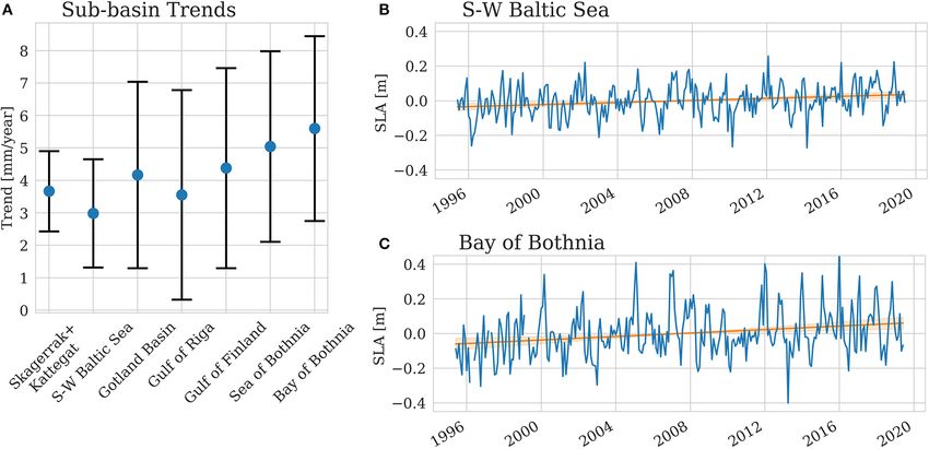
Passaro et al.                                                                                                                      Absolute Baltic Sea Level Trends

 FIGURE 4 | SL trends (A) and corresponding uncertainties (B) estimated by altimetry (shading) and TGs (circles) from May 1995 to May 2019. TGs are corrected for
 the GIA using the NKG2016 model. Uncertainties are reported as 95% confidence interval.

the South West of the Baltic Sea (S-W) to the Gotland Basin,                        the comparability between trends from altimetry and from TGs
and from the Gotland Basin to the Bay of Bothnia and the Gulf                       improves by 9% using the Baltic+ data in terms of root mean
of Finland.                                                                         square of the differences. All the altimetry dataset show a median
   By retrieving the SL information from the leads within sea-ice                   of the trends that is about 0.2 mm/yr lower than in the TG
in winter, we are able to extend the analysis to areas characterised                records. We acknowledge that the nonlinear elastic uplift from
by seasonal sea-ice coverage, i.e., Bay of Bothnia and Gulf of                      present day deglaciation, which is not taken in consideration by
Finland. Nevertheless, gaps are still present in such regions along                 the GIA model, may affect the bias, although GIA has been shown
the coast. Other remaining gaps involve locations in the Danish                     to be the dominating source of vertical deformation in the region
Archipelago, where the predominant presence of land within the                      (Ludwigsen et al., 2020).
search radius of each grid point hinders the possibility to find                        Figure 4B also shows the uncertainty of the computed trends.
enough data in particular during years in which few altimeters                      This is a purely statistical function of the number of samples in
were in orbit. Finally, our SL analysis does not provide results                    the time series and their SL variability, taking in to consideration
in some parts of the Turku Archipelago (south-western Finnish                       the serial correlation. The same method is used also to estimate
coast). The presence of numerous islets in this area means that                     the uncertainty of the trend estimated from TGs, which also do
the vast majority of SL retrieval are located at distances below                    not have an uncertainty value associated to each measurement.
1 km from the nearest land. This is well below the possibilities                    This is in line with most of the studies estimating trends
of any LRM altimeter, even using coastal retracking to avoid                        from altimetry measurements, for example (Benveniste et al.,
land contamination.                                                                 2020). The possibility to associate an uncertainty to the single
   These data gaps could be artificially mitigated by means of                      altimetry measurement has been explored by (Ablain et al.,
heavier interpolation and different weighting in the gridding                       2016) and analysed in the BS by Madsen et al. (2019), but
process, nevertheless the choice in this study is to avoid                          requires a large amount of assumptions concerning every single
generating information that is indeed not available. The                            correction added to the altimetric range. Nevertheless, our
comparison of the agreement between the SL trends from                              statistical uncertainties show a similar pattern and range of the
different altimetry dataset and TGs presented in Figure 5 is a                      ones shown in Madsen et al. (2019).
proof of the validity of our solution. In the histograms, the SL                        By grouping the grid points according to their location,
trend estimates from the TGs are compared with the closest                          Figure 6 displays the averaged SL trends of each sub-basin
estimates from altimetry using data from this study (Figure 5A)                     with their statistical uncertainty. In Figures 6B,C, the monthly
and data from CMEMS (Figure 5B, Taburet et al., 2019). The                          time series for the Bay of Bothnia and the S-W are shown as
time series are restricted to the interval May 1995-December 2018                   examples, since they present the largest discrepancies in the
to enable the comparison with CMEMS. In Figure 5C, the length                       linear trend estimations. The rise in SL is statistically significant
of the time series of this study is May 1995–December 2015, to                      in all sub-basins. The spatial variation of the best estimate
enable the comparison with the gridded product of the SLCCI                         of the linear trend is confirmed, although the uncertainties
(Figure 5D, Legeais et al., 2018). In both pairs of comparison,                     due to the larger variability of the SL time series in most

Frontiers in Marine Science | www.frontiersin.org                               8                                              May 2021 | Volume 8 | Article 647607
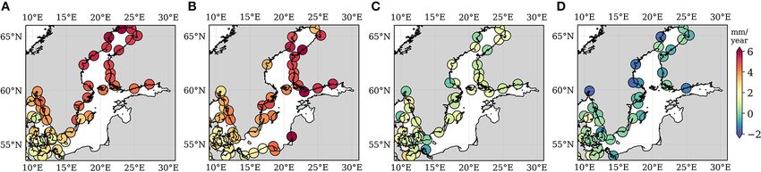
Passaro et al.                                                                                                                          Absolute Baltic Sea Level Trends

 FIGURE 5 | Histograms of the differences in estimated SL trends from gridded altimetry (SAT) and TGs, compared using the closest point. Each panel correspond to
 different SAT dataset: the altimetry dataset from May 1995 to December 2018 developed in this study (A, Baltic+), the altimetry dataset from May 1995 to December
 2018 CMEMS (B, Copernicus), the altimetry dataset from May 1995 to December 2015 developed in this study (C, Baltic+), the altimetry dataset from May 1995 to
 December 2015 of the SLCCI (D, SLCCI).

 FIGURE 6 | (A) SL trends from gridded altimetry averaged across different sub-basins of the BS from May 1995 to May 2019. Corresponding uncertainties are
 reported as black error bars. (B,C) Monthly SL time series of the S-W Baltic Sea and the Bay of Bothnia. The linear trend is shown as a red line, with the shading
 representing its uncertainty.

of the sub-basins cannot ensure statistical significance to this                       spatial variation in the trend is less pronounced in summer. Due
assertion yet.                                                                         to the relatively short duration of the time series, the seasonal
   Figure 7 shows the trends in SL considering only the                                trend uncertainties are comparatively large. Thus, we investigate
winter months (Figures 7A,C) and only the summer months                                whether a similar pattern can also be found in TG records, which
(Figures 7B,D). Positive trends are found in the winter SL, with                       spans much longer periods than the altimetry time series.
a difference of over 4 mm/year comparing the winter trends in                             Figures 8A–D report the best estimate of the linear trends in
their minimum and maximum values. A similar gradient in SL                             SL from the longest TG time series in the region, spanning from
trend estimates is seen for the full time series in Figure 4A. This                    1920 to 2020 at intervals of 25 years. Indeed, the same gradient

Frontiers in Marine Science | www.frontiersin.org                                  9                                               May 2021 | Volume 8 | Article 647607
Passaro et al. Absolute Baltic Sea Level Trends
FIGURE 7 | SL trends with uncertainties from gridded altimetry computed using only the winter months (December, January, and February, A,C) and the summer
months (June, July, and August, B,D).
of about 4 mm/yr in SL trend estimates from altimetry across the (as described in section 2.3.2). Figures 9A,D show the spatial
basin is observed in the most recent TG record (Figure 8A). It patterns of the first and second EOFs. We find that 87.4% of
is observed not only that the SL rise in the BS is evident in the the variance in the entire domain is explained by the first EOF,
last 50 years, but also that the spatial gradient in trends has been which is associated with a uniform SL pattern across the basin.
increasing in time. The second EOF, while representing 3.1% of the variance, is
In the next section, we analyse the possible role of wind connected to a SL variability with a strong gradient from S-
patterns and the NAO in shaping this spatial gradient. W toward Bay of Bothnia and Gulf of Finland, generating SL
anomalies of opposite sign.
3.2. Discussion To characterise these two modes, we correlate the
3.2.1. Relationships With Wind Pattern accompanying PC to the zonal (U) and meridional
To analyse the spatial and temporal pattern of SL variability and (V) components of the surface wind from the ERA5
how they differ locally across the basin, we perform an EOF reanalyses (Hersbach et al., 2020). The results displayed in
analysis on the deseasoned altimetry time series at each grid point Figures 9B,C,E,F, show that the PC1 is correlated with U in the
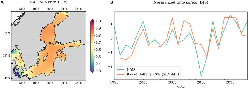
Frontiers in Marine Science | www.frontiersin.org 10 May 2021 | Volume 8 | Article 647607Passaro et al. Absolute Baltic Sea Level Trends FIGURE 8 | SL trends from TGs computed at 25-year intervals from 1920 to 2020. (A) Linear trends 2020–1995, (B) linear trends 1995–1970, (C) linear trends 1970–1945, (D) linear trends 1945–1920. FIGURE 9 | (A,D) Empirical orthogonal functions of SL variability expressed as correlation of their corresponding PC against the SL time series at each grid point. (B,C) Correlation between the first PC of SL variability and the zonal (U) and meridional (V) component of the surface winds. (E,F) Same for the second PC. South of the basin, with the correlation degrading toward North. component of the wind and for the sum of the two components The predominance of the zonal component in shaping the SL is presented, with its uncertainty. The average variance explained variance of the region is in accordance with previous studies, for is 31% by U and 2% by V, but the latter explains over 15% of example Johansson et al. (2014). PC2 is instead well described the variance in the Bay of Bothnia (not shown). Despite the by the variability of V, with correlation values over 0.5 in all our high variance explained, the U regression shows a very small, region of study. homogenous trend in the whole BS, while V is responsible for To further study how the wind variability may affect the a gradient of over 1 mm/yr from South to North. Although a estimates of SL trend during the altimetry era, we perform a conclusive statement with statistical relevance cannot be drawn, multiple regression analysis of the SL time series using the U given the uncertainties, both EOF and regression analysis point and V wind components (as described in section 2.3.3). We out to the same role of the meridional wind component to consider the large scale wind field by spatially averaging the shape a North-South imbalance in the SL anomalies. Recently, monthly wind speed over the entire domain. The results are spatial gradients of the SL trend within the BS have been shown in Figure 10, in which the explained trend for each attributed, based on circulation models, to an increase in the Frontiers in Marine Science | www.frontiersin.org 11 May 2021 | Volume 8 | Article 647607
Passaro et al. Absolute Baltic Sea Level Trends
FIGURE 10 | Trends resulting from the regression of the zonal (U, A) and meridional (V, B) component of the surface winds on the SL time series. (C) Shows the trend
obtained summing the two components of the regression. (D–F) Show the corresponding uncertainties of the respective trend estimations in (A–C).
days of westerly winds, which increase transport toward the east winter months is plotted against the NAO index. The correlation
(Gräwe et al., 2019). Our analysis suggests that the meridional between the two curves is 0.71. From the comparison it is seen
wind component also affects the differences in SL trend among that positive NAO phases are related to winters in which the SLA
the sub-basins. are higher in Bay of Bothnia than in S-W. As seen in the next
section, this is linked to the action of stronger southerlies and
3.2.2. Relationships With North-Atlantic Oscillation westerlies winds during positive NAO phases, which push the
The large scale variability of both SL and wind patterns in our water north and east of the basin through Ekman transport. The
area of study can be well-described using teleconnections. There intensity of the NAO phase, which is linked to the wind forcing
is a strong agreement that the NAO is the leading mode of (Dangendorf et al., 2013), is here shown to drive differences of
atmospheric circulation in the region (Andersson, 2002; Jevrejeva SLA at a sub-basin scale in the BS, with interannual variations
et al., 2005). Interconnections with other climate patterns and the that have an effect on the linear trend of the SL estimated on
corresponding indices have been shown to play a role in the area, time series spanning two decades of observations. In particular,
such as the East Atlantic (EAP) pattern, Scandinavian (SCAN) as seen in Figure 10, the effect of the positive NAO phases in
pattern (Chafik et al., 2017) and the BS and North Sea Oscillation our period of observation results in a wind-related SL trend
index (BANOS) (Karabil et al., 2018). increasing toward north.
We focus on the local effects of NAO variability, since
the relationship of NAO to the Baltic SL variability has been
previously reported to be spatially heterogeneous (Jevrejeva 3.2.3. Ekman Currents
et al., 2005 with TG observations, Stephenson et al., 2006 with Winds affect the surface circulation of water masses through
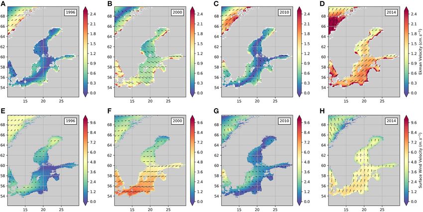
global models). Figure 11A shows that in the altimetry era the Ekman transport. We show in Figure 12 the average winter
correlation between the SL variability and the NAO index is wind speed direction (Figures 12E–H) and the resultant Ekman
dominant in winter, as expected, and uniform in the whole currents (Figures 12A–D) in selected winter seasons to observe
domain except for the S-W. the mechanism that may regulate the SL differences among
The possibility given by our dataset to observe local SL different sub-basins within the BS. The years are chosen based on
changes in winter in the sea-ice covered areas allow a basin- the highest and lowest differences between the winter SLA of Bay
wide comparison of the Bay of Bothnia against the S-W, which of Bothnia and the S-W as reported in Figure 11B. We analyse
present the largest discrepancies in the linear trend estimations. the Ekman transport at 15 m depth from the GlobCurrent ocean
In Figure 11B, the difference in SL (Bay of Bothnia–S-W) in the product (Rio et al., 2014). The Ekman currents are distributed on
Frontiers in Marine Science | www.frontiersin.org 12 May 2021 | Volume 8 | Article 647607Passaro et al. Absolute Baltic Sea Level Trends FIGURE 11 | (A) Correlation of the NAO index with SLA from gridded altimetry. (B) Normalized time series of NAO index (green) and SLA difference between Bay of Bothnia and S-W sub-basins (orange). Each point represents the time average of the quantities of the winter months December, January, and February. FIGURE 12 | Velocity of the Ekman currents (A–D) and surface wind velocity (E–H) during the winters of four selected years. The arrows represent the direction of the velocity vectors and are scaled according to their magnitude. a 1/4 of a degree grid and they are derived using wind stress from GlobCurrent product, we are mostly interested in the effect of the ECMWF, Argo floats and in-situ surface drifter data. Ekman currents in the southern part of the domain. The results When considering these results, we are dropping the are consistent with the Ekman transport pushing the surface hypothesis of a fully developed Ekman spiral, in which case waters to the right of the wind direction. the transport would be perpendicular to the wind direction. Winters with SLA higher in Bay of Bothnia than in S-W (e.g., Nevertheless, given the low depths of the S-W of the BS, the 15 2000, 2014) are either characterised by strong westerlies in S-W m-depth Ekman transport should be a good approximation at whose intensity decrease toward the North (e.g., 2000), or by a least in this sub-basin. Since the Bay of Bothnia is covered by marked southerly component of the wind (e.g., 2014). Years in sea-ice for most of the winters, which hinders formation of an which the differences are very low, or even flip (e.g., 1996, 2010) Ekman spiral, and since sea-ice is not taken into account in the are characterised by much lower wind speed. Frontiers in Marine Science | www.frontiersin.org 13 May 2021 | Volume 8 | Article 647607
Passaro et al.                                                                                                      Absolute Baltic Sea Level Trends

   In conclusion, the years in which the winter SLA in the Bay               in the exploitation of altimetry in the coastal zone are focused
of Bothnia are higher than in the S-W are characterised by a                 on the analysis of along-track data, this work for the first time
strong Ekman transport, which affects the sea-ice free part of the           employs a coastal-dedicated reprocessing to produce gridded sea
domain. This mechanism fails during the negative NAO phases,                 level data. Moreover, we have demonstrated that such techniques
directly affecting the SL difference between the two sub-basins.             are able to obtain reliable sea level time series also in areas
                                                                             and seasons interested by sea-ice coverage. The BS has proved
4. CONCLUDING REMARKS                                                        to be an excellent region to explore these issues concerning
                                                                             coastal altimetry. Using the best practice advances developed
This study analysed the SL trend in the BS during most of the                here, comparative analyses can be conducted in more tide-prone
altimetry era (1995–2019). A new reprocessing in the framework               regions to test the further applicability of our approach.
of the ESA Baltic SEAL project enables the retrieval of more data
in the coastal zone and among sea-ice. A trend analysis based on             DATA AVAILABILITY STATEMENT
this dataset improves the agreement with trends estimated using
GIA-corrected TGs (Figure 5). The information retrieved from                 The datasets presented in this study can be found in
the leads among sea-ice covered areas enhances the possibility               online repositories. The names of the repository/repositories
to study SL variability and its differences across the basin during          and accession number(s) can be found at: http://balticseal.eu/
winter, which is the season with the largest SL rise in our                  data-access/.
observation period (Figure 7).
    The absolute SL rise is statistically significant in the entire          AUTHOR CONTRIBUTIONS
domain, since the uncertainties are lower than the trend estimates
(Figure 4). Differences in trends among the sub-basins are not               MP designed the study, wrote the manuscript, and was the
statistically significant, but are seen in both the TGs and the              principal investigator of the research group. He was also the
altimetry dataset (Figure 6).                                                author of the retracking algorithm and of the sea state bias
    The absolute SL rise is a year-round phenomenon, although                correction developed for this study. FM was responsible for the
trends are higher in winter than in summer. The gradient in                  classification and the gridding. He was the main responsible
SL rise across the basin mainly occurs during winter (Figure 7).             for the altimetry database organisation, with CS and DD. FM
SL differences between the North and the South West of the BS                also contributed in the coordination of the activities of the
are shown to be well-correlated with the NAO index in winter                 research group. JO was responsible for the trend and sea level
(Figure 11). In particular, winter positive NAO phases trigger               variability estimation and interpretation. DD was responsible for
lower SL anomalies in the S-W, as strong south-westerly winds                the multi-mission calibration. AA and OA were responsible for
transport surface water away from the sub-basin (Figure 12).                 the mean sea surface used to obtain the sea level anomalies.
    The NAO drives not only the SL in the entire domain, but                 MH-D contributed in the interpretation of the sea level trends.
is shown to also affect internal sub-basin gradients. A part of              FS provided the basic resources making the study possible and
it can be explained by wind forcing, which accounts on average               coordinates the activities of the research group at TUM. RS
for about 40% of the SL variability. Other factors can contribute            helped in the coordination of the research group and reviewed
to the observed spatial gradient of the SL trend, which we plan              the manuscript. JH, KM, and IR contributed to the interpretation
to consider in a future study. Karabil et al. (2018) for example             of the results. LR, JS, and LT were responsible for the validation
observes that a possible driver can be the freshwater flux, but              of the along-track data. MP, MR, and JB conceptualized the
this would be particularly pronounced in summertime, therefore               research project. MR and JB reviewed the manuscript and all
would not explain the larger trend differences found in winter.              deliverables of the research project and supported the validation
The increasing use of GRACE data to compute mass SL changes                  activities of the ALES+ SAR retracking algorithm. All authors
at a regional scale (Kusche et al., 2016) and the availability of sea        read, commented, and reviewed the final manuscript.
surface temperature and salinity datasets can be combined with
measurements from the Argo floats (Guinehut et al., 2004; Boutin             ACKNOWLEDGMENTS
et al., 2013) (particularly in a low-depth basin like the BS). This
suggests that a regional SL budget based on observational data               This study is a contribution to the ESA Baltic+ Sea Level
shall be the subject of a future study and the next step to increase         project (ESA AO/1-9172/17/I-BG - BALTIC +, contract number
our knowledge of the Baltic SL variability and drivers.                      4000126590/19/I/BG). We use the python distribution eofs
    This study highlights the value of developing regionalised SL            (Dawson, 2016) for computation of the EOF. We used the Hector
products, using satellite altimetry measurements. It has improved            software (Bos et al., 2013) to estimate the trend uncertainties
the efficacy of retrieving meaningful SL observations from                   from MLE and study the impact of different noise models, as
areas featuring complex coastlines, and those affected by sea-ice            described in section 2.3.1. We thank Samantha Royston for the
contamination of the altimeter footprint. While current efforts              useful discussion concerning noise models in time series analysis.

Frontiers in Marine Science | www.frontiersin.org                       14                                      May 2021 | Volume 8 | Article 647607
Passaro et al. Absolute Baltic Sea Level Trends
REFERENCES Guinehut, S., Le Traon, P., Larnicol, G., and Philipps, S. (2004). Combining Argo
and remote-sensing data to estimate the ocean three-dimensional temperature
Ablain, M., Legeais, J., Prandi, P., Marcos, M., Fenoglio-Marc, L., Dieng, H., et al. fieldsÑa first approach based on simulated observations. J. Mar. Syst. 46, 85–98.
(2016). Satellite altimetry-based sea level at global and regional scales. Surveys doi: 10.1016/j.jmarsys.2003.11.022
Geophys. 38, 7–31. doi: 10.1007/s10712-016-9389-8 Hastie T., Tibshirani R., Friedman J. (2009). The Elements of Statistical Learning,
Akaike, H. (1998). Information Theory and an Extension of the Maximum Vol. 2. New York, NY: Springer-Verlag. doi: 10.1007/978-0-387-84858-7
Likelihood Principle. New York, NY: Springer New York, 199–213. Hayne, G. S. (1980). Radar altimeter mean return waveforms from near-normal-
doi: 10.1007/978-1-4612-1694-0_15 incidence ocean surface scattering. IEEE Trans. Antenn. Propag. 28, 687–692.
Andersson, H. C. (2002). Influence of long-term regional and large-scale doi: 10.1109/TAP.1980.1142398
atmospheric circulation on the Baltic sea level. Tellus A 54, 76–88. Hersbach, H., Bell, B., Berrisford, P., Hirahara, S., Horányi, A., Mu noz-Sabater, J.,
doi: 10.3402/tellusa.v54i1.12125 et al. (2020). The ERA5 global reanalysis. Q. J. R. Meteorol. Soc. 146, 1999–2049.
Beckley, B. D., Callahan, P. S., Hancock, D. III, Mitchum, G., and Ray, R. doi: 10.1002/qj.3803
(2017). On the Cal-Mode correction to TOPEX satellite altimetry and its effect Jevrejeva, S., Moore, J., Woodworth, P., and Grinsted, A. (2005). Influence
on the global mean sea level time series. J. Geophys. Res. 122, 8371–8384. of large-scale atmospheric circulation on European sea level: results
doi: 10.1002/2017JC013090 based on the wavelet transform method. Tellus A 57, 183–193.
Benveniste, J., Birol, F., Calafat, F., Cazenave, A., Dieng, H., Gouzenes, doi: 10.3402/tellusa.v57i2.14609
Y., et al. (2020). (The Climate Change Initiative Coastal Sea Level Johansson, M. M., Pellikka, H., Kahma, K. K., and Ruosteenoja, K. (2014). Global
Team) Coastal sea level anomalies and associated trends from Jason sea level rise scenarios adapted to the finnish coast. J. Mar. Syst. 129, 35–46.
satellite altimetry over 2002-2018. Sci. Data 7:357. doi: 10.1038/s41597-020- doi: 10.1016/j.jmarsys.2012.08.007
00694-w Karabil, S., Zorita, E., and Hünicke, B. (2018). Contribution of atmospheric
Benveniste, J., Cazenave, A., Vignudelli, S., Fenoglio-Marc, L., Shah, R., Almar, R., circulation to recent off-shore sea-level variations in the Baltic sea and the north
et al. (2019). Requirements for a coastal hazards observing system. Front. Mar. sea. Earth Syst. Dyn. 9, 69–90. doi: 10.5194/esd-9-69-2018
Sci. 6:348. doi: 10.3389/fmars.2019.00348 Kusche, J., Uebbing, B., Rietbroek, R., Shum, C., and Khan, Z. (2016).
Bos, M. S., Fernandes, R. M. S., Williams, S. D. P., and Bastos, L. (2013). Fast Sea level budget in the Bay of Bengal (2002-2014) from GRACE
error analysis of continuous GNSS observations with missing data. J. Geod. 87, and altimetry. J. Geophys. Res. 121, 1194–1217. doi: 10.1002/2015JC0
351–360. doi: 10.1007/s00190-012-0605-0 11471
Bosch, W., Dettmering, D., and Schwatke, C. (2014). Multi-mission cross- Landskron, D., and Böhm, J. (2018). VMF3/GPT3: refined discrete and
calibration of satellite altimeters: constructing a long-term data record for empirical troposphere mapping functions. J. Geodesy 92, 349–360.
global and regional sea level change studies. Remote Sens. 6, 2255–2281. doi: 10.1007/s00190-017-1066-2
doi: 10.3390/rs6032255 Legeais, J.-F., Ablain, M., Zawadzki, L., Zuo, H., Johannessen, J. A., Scharffenberg,
Boutin, J., Martin, N., Reverdin, G., Yin, X., and Gaillard, F. (2013). Sea surface M. G., et al. (2018). An improved and homogeneous altimeter sea level
freshening inferred from SMOS and ARGO salinity: impact of rain. Ocean Sci. record from the ESA climate change initiative. Earth Syst. Sci. Data 10:281.
9, 183–192. doi: 10.5194/os-9-183-2013 doi: 10.5194/essd-10-281-2018
Brown, G. (1977). The average impulse response of a rough surface Leppäranta, M., and Myrberg, K. (2009). Physical Oceanography of the Baltic Sea.
and its applications. IEEE Trans. Anten. Propag. 25, 67–74. Springer Science & Business Media. doi: 10.1007/978-3-540-79703-6
doi: 10.1109/TAP.1977.1141536 Ludwigsen, C. A., Khan, S. A., Andersen, O. B., and Marzeion, B. (2020). Vertical
Carrere, L., Lyard, F., Cancet, M., and Guillot, A. (2015). “FES 2014, a new tidal Land Motion from present-day deglaciation in the wider Arctic. Geophys. Res.
model on the global ocean with enhanced accuracy in shallow seas and in the Lett. 47:e2020GL088144. doi: 10.1029/2020GL088144
arctic region,” in EGU General Assembly Conference Abstracts, Vol. 17 (Wien), Madsen, K. S., Höyer, J. L., Suursaar, Ü., She, J., and Knudsen, P. (2019). Sea level
5481. trends and variability of the Baltic sea from 2d statistical reconstruction and
Celebi, M. (2014). Partitional Clustering Algorithms. EBL-Schweitzer. Springer altimetry. Front. Earth Sci. 7:243. doi: 10.3389/feart.2019.00243
International Publishing. doi: 10.1007/978-3-319-09259-1 Müller, F. L., Dettmering, D., Bosch, W., and Seitz, F. (2017). Monitoring the arctic
Chafik, L., Nilsen, J. E. Ø., and Dangendorf, S. (2017). Impact of north atlantic seas: How satellite altimetry can be used to detect open water in sea-ice regions.
teleconnection patterns on northern European sea level. J. Mar. Sci. Eng. 5:43. Remote Sens. 9:551. doi: 10.3390/rs9060551
doi: 10.3390/jmse5030043 Olivieri, M., and Spada, G. (2016). Spatial sea-level reconstruction in the Baltic Sea
Collecte Localisation Satellites (CLS). Dynamic Atmospheric Corrections Are and in the Pacific Ocean from tide gauges observations. Ann. Geophys. 59:0323.
Produced by CLS Space Oceanography Division Using the MOG2D Model From doi: 10.4401/ag-6966
Legos and Distributed by AVISO+, With Support from CNES. AVISO+. Passaro, M., Dinardo, S., Quartly, G. D., Snaith, H. M., Benveniste, J., Cipollini,
Dangendorf, S., Mudersbach, C., Wahl, T., and Jensen, J. (2013). Characteristics P., et al. (2016). Cross-calibrating ALES Envisat and Cryosat-2 Delay-Doppler:
of intra-, inter-annual and decadal sea-level variability and the role of a coastal altimetry study in the Indonesian Seas. Adv. Space Res. 58, 289–303.
meteorological forcing: the long record of Cuxhaven. Ocean Dyn. 63, 209–224. doi: 10.1016/j.asr.2016.04.011
doi: 10.1007/s10236-013-0598-0 Passaro, M., Mueller, F., and Dettmering, D. (2020a). Baltic+ SEAL:
Dawson, A. (2016). EOFS: a library for EOF analysis of meteorological, Algorithm Theoretical Baseline Document (ATBD). Technical report
oceanographic, and climate data. J. Open Res. Softw. 4:e14. doi: 10.5334/jors.122 delivered under the Baltic+ SEAL project, European Space Agency.
Dettmering, D., Wynne, A., Müller, F. L., Passaro, M., and Seitz, F. (2018). doi: 10.5270/esa.BalticSEAL.ATBDV1.1
Lead detection in polar oceansÑA comparison of different classification Passaro, M., Nadzir, Z., and Quartly, G. D. (2018b). Improving the precision
methods for Cryosat-2 SAR data. Remote Sens. 10:1190. doi: 10.3390/rs100 of sea level data from satellite altimetry with high-frequency and
81190 regional sea state bias corrections. Remote Sens. Environ. 218, 245–254.
Fernandes, M. J., and Lazaro, C. (2016). GPD+ wet tropospheric corrections doi: 10.1016/j.rse.2018.09.007
for cryosat-2 and GFO altimetry missions. Remote Sens. 8:851. Passaro, M., Restano, M., Sabatino, G., C., O., and J, B. (2020b). “The ALES+ SAR
doi: 10.3390/rs8100851 service for Cryosat-2 and Sentinel-3 at ESA GPOD,” in Presented at the Ocean
Fernandes, M. J., Lázaro, C., Ablain, M., and Pires, N. (2015). Improved wet path Surface Topography Science Team (OSTST) Meeting. Available online at: https://
delays for all esa and reference altimetric missions. Remote Sens. Environ. 169, meetings.aviso.altimetry.fr/index.html
50–74. doi: 10.1016/j.rse.2015.07.023 Passaro, M., Rose, S., Andersen, O., Boergens, E., Calafat, F., and J, B. (2018a).
Gräwe, U., Klingbeil, K., Kelln, J., and Dangendorf, S. (2019). Decomposing mean ALES+: Adapting a homogenous ocean retracker for satellite altimetry to
sea level rise in a semi-enclosed basin, the Baltic sea. J. Clim. 32, 3089–3108. sea ice leads, coastal and inland waters. Remote Sens. Environ. 211, 456–471.
doi: 10.1175/JCLI-D-18-0174.1 doi: 10.1016/j.rse.2018.02.074
Frontiers in Marine Science | www.frontiersin.org 15 May 2021 | Volume 8 | Article 647607You can also read