Spatial and temporal analysis of extreme storm-tide and skew-surge events around the coastline of New Zealand - NHESS
←
→
Page content transcription
If your browser does not render page correctly, please read the page content below
Nat. Hazards Earth Syst. Sci., 20, 783–796, 2020
https://doi.org/10.5194/nhess-20-783-2020
© Author(s) 2020. This work is distributed under
the Creative Commons Attribution 4.0 License.

Spatial and temporal analysis of extreme storm-tide and skew-surge
events around the coastline of New Zealand
Scott A. Stephens1 , Robert G. Bell1 , and Ivan D. Haigh2
1 National
         Institute of Water and Atmospheric Research, P.O. Box 11 115, Hamilton 3251, New Zealand
2 Oceanand Earth Science, National Oceanography Centre, University of Southampton, European Way,
Southampton, SO14 3ZH, UK

Correspondence: Scott A. Stephens (Scott.Stephens@niwa.co.nz)

Received: 23 October 2019 – Discussion started: 28 November 2019
Accepted: 10 February 2020 – Published: 24 March 2020

Abstract. Coastal flooding is a major global hazard, yet few      findings have important implications for flood management,
studies have examined the spatial and temporal character-         emergency response and the insurance sector, because im-
istics of extreme sea level and associated coastal flooding.      pacts and losses may be correlated in space and time.
Here we analyse sea-level records around the coast of New
Zealand (NZ) to quantify extreme storm-tide and skew-surge
frequency and magnitude. We identify the relative magnitude
of sea-level components contributing to 85 extreme sea level      1   Introduction
and 135 extreme skew-surge events recorded in NZ since
1900. We then examine the spatial and temporal clustering         Coastal flooding is a major global hazard with historical
of these extreme storm-tide and skew-surge events and iden-       events killing hundreds of thousands of people and causing
tify typical storm tracks and weather types associated with       billions of dollars in damage to property and infrastructure
the spatial clusters of extreme events. We find that most ex-     (e.g. Lagmay et al., 2015; Needham et al., 2015; Haigh et
treme storm tides were driven by moderate skew surges com-        al., 2016). Globally, it has been estimated that up to 310
bined with high perigean spring tides. The spring–neap tidal      million people are already exposed to a 1 in 100-year flood
cycle, coupled with a moderate surge climatology, prevents        from the sea (Jongman et al., 2012; Hinkel et al., 2014; Muis
successive extreme storm-tide events from happening within        et al., 2016). In New Zealand this includes 72 000 people –
4–10 d of each other, and generally there are at least 10 d       1.5 % of the population (Paulik et al., 2019, 2020). This will
between extreme storm-tide events. This is similar to find-       get worse, since without adaptation, it has been estimated
ings from the UK (Haigh et al., 2016), despite NZ having          that 0.2 %–4.6 % of global population will be flooded annu-
smaller tides. Extreme events more commonly impacted the          ally under 25–123 cm (RCP2.6–RCP8.5) of global mean sea-
east coast of the North Island of NZ during blocking weather      level rise (SLR; Hinkel et al., 2014). Improved understanding
types, and the South Island and west coast of the North Is-       of extreme sea level and coastal flooding events is therefore
land during trough weather types. The seasonal distribution       important.
of both extreme storm-tide and skew-surge events closely fol-        To understand and manage their risk exposure, central
lows the seasonal pattern of mean sea-level anomaly (MSLA)        government agencies, environmental and emergency man-
– MSLA was positive in 92 % of all extreme storm-tide             agers and the insurance and financial sectors, all require
events and in 88 % of all extreme skew-surge events. The          knowledge of the likely frequency and magnitude of extreme
strong influence of low-amplitude ( − 0.06 to 0.28 m) MSLA        storm-tide events and their clustering in time and space.
on the timing of extreme events shows that mean sea-level         Studies have quantified the frequency and magnitude of ex-
rise (SLR) of similarly small height will drive rapid increases   treme sea levels at regional (e.g. Bernier and Thompson,
in the frequency of presently rare extreme sea levels. These      2006; I. Haigh et al., 2010; I. D. Haigh et al., 2010, 2014) and
                                                                  global (e.g. Menéndez and Woodworth, 2010; Muis et al.,

Published by Copernicus Publications on behalf of the European Geosciences Union.
784 S. A. Stephens et al.: Spatial and temporal analysis
2016) scales, but, other than Haigh et al. (2016), recognition MSLA. Since skew surge is the height difference between
and analysis of spatial and temporal extreme sea-level char- a storm-tide peak and the nearest predicted high tide, then
acteristics and associated coastal flooding is lacking globally. skew surge contains a component of both storm surge plus
Haigh et al. (2016) provided an analysis of spatial and tempo- MSLA.
ral extreme sea-level (storm-tide) characteristics for the UK NZ tides are mostly meso-tidal (2–4 m tidal range) but
coastline. In this paper we undertake a similar analysis for the with some micro-tidal (< 2 m range) locations (e.g. Welling-
New Zealand (NZ) coastline, contributing to a growing un- ton). The tidal regime is mixed semi-diurnal, experiencing
derstanding of spatial and temporal extreme sea-level char- two high tides per day of which one high tide is larger than
acteristics worldwide for different tidal and storm contexts. the other. Tides are larger on the west coast where the semi-
In the past, relatively few NZ sea-level records have been diurnal signal is stronger and there is a strong fortnightly
included in global extreme sea-level studies (e.g. Wahl et spring–neap cycle. Tides are smaller on the east coast where
al., 2017) whose focus was on global intra-comparisons and an amphidrome in the diurnal S2 constituent leads to a more
trends. Therefore, here we provide a comprehensive assess- noticeable monthly perigean influence in the peak tides (Wal-
ment of extreme sea level and skew surge in NZ based on a ters et al., 2001). Tides flow west to east through the con-
more extensive tide gauge dataset (with on-average records stricted Cook Strait (which separates the North Island and the
of 30 years in length). We use sea-level gauge records to South Island, Fig. 1), and the constriction causes the largest
quantify the frequency–magnitude distribution of extreme tides to occur near Nelson (site 22, Fig. 1) and the smallest
sea level and skew surges. Skew surge is the height difference tides at Wellington (site 11, Fig. 1).
between a sea-level (storm-tide) peak and the nearest high NZ does not experience tropical cyclones (hurricanes) and
tide. We also examine the influence of the mean sea-level has a relatively deep and narrow continental shelf and so does
anomaly (MSLA) on the timing of extreme storm-tide events. not experience very large storm surges on a global scale – the
MSLA is derived from the low-frequency non-tidal residual semi-diurnal tides dominate sea-level variability and storm
sea level (Merrifield et al., 2013), which is dominated by surges are limited to mostly < 0.5 m, which is approximately
seasonal heating and cooling of the sea (Bell and Goring, 25 % of the average tidal range (Stephens et al., 2014). Rueda
1998; Boon, 2013) and inter-annual climate cycles such as et al. (2017) classify NZ’s coastal flood hazard climate as be-
El Niño–Southern Oscillation (Goring and Bell, 1999) and ing “lightly unbounded” (extreme storm-tide shape parame-
is often not considered in extreme storm-tide analyses be- ter weakly positive), “macro-level” (total water level ≥ 1 m),
cause in most places it is small compared to tide and skew “highly variable” (high interannual variability) and “tide-
surge – we show that it has an important influence on the dominant” (tidal range dominates the total water level height
timing of extreme storm-tide and skew-surge events in NZ. compared to storm surge and wave set-up).
We analyse the spatial and temporal clustering of extreme
storm-tide and skew-surge events and identify typical storm
tracks and weather types associated with spatial clusters of 3 Data and methods
extreme events.
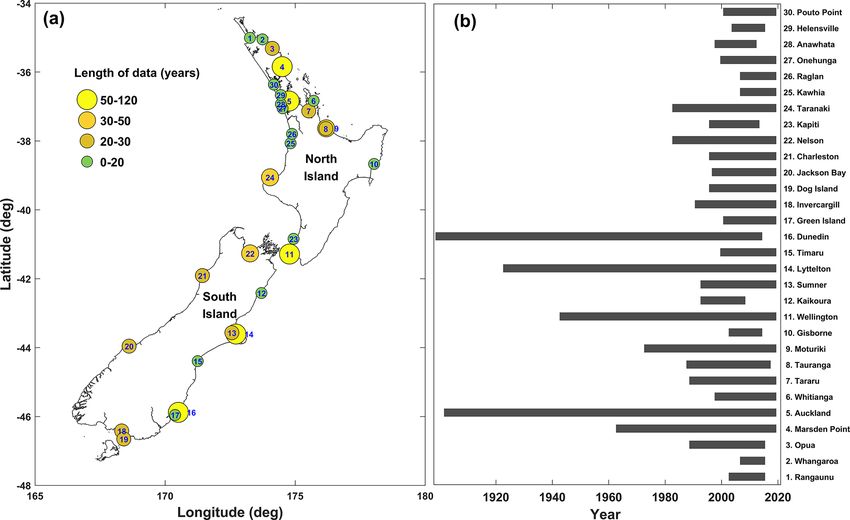
We analysed sea-level records from 30 locations in NZ
(Fig. 1). The duration of the records ranged from 6 to
2 New Zealand storm-tide characteristics 115 years with a mean and median of 31 and 20 years re-
spectively, with mostly concurrent records since the early
Tsunami and land subsidence aside, there are several mete- 1990s. The sea-level records were quality-analysed to re-
orological and astronomical influences on sea level that can move any spikes, timing errors, or datum shifts but leaving
combine in a number of ways to inundate low-lying coastal any data gaps. Tide gauge stations globally are typically lo-
margins: the height of mean sea level (MSL) relative to a lo- cated in protected embayments, which limits the direct im-
cal datum or landmark, astronomical tides (referred to hence- pact of wind waves relative to open coastlines, but storm
forth simply as tide), synoptic weather-induced storm surge, surges (and skew surges) generally are well sampled by tide
MSLA (caused by seasonal, interannual and inter-decadal gauges (e.g. Merrifield et al., 2013), provided no seiching oc-
climate variability), long-term change in MSL through SLR, curs, or, if it does occur, the sampling rate is fine enough to
and wave set-up and run-up. We use the term MSLA in resolve the seiche. The NZ sea-level records analysed here
recognition that the anomaly is calculated relative to MSL, are from a variety of locations including wave-exposed open
after MSL and any long-term MSL trend has been removed coast, inside port breakwaters, or mounted on wharves in-
(described later). It is common to treat the wave-induced side estuaries, so they have different levels of wave exposure.
set-up and run-up separately from the still (non-wave) wa- The sampling frequency varies between and within individ-
ter level because sea-level gauges are usually placed inside ual records, from 1 min up to 1 h sampling intervals. At some
harbours to minimize the effects of wave set-up and run- sites far infragravity waves of > 2 min and several decimetres
up. Here we define the term “storm tide” as the total water amplitude are observed in the 1 min data during local or re-
level above MSL from the sum of tide plus storm surge plus mote storm events (Thiebaut et al., 2013), and tsunami events
Nat. Hazards Earth Syst. Sci., 20, 783–796, 2020 www.nat-hazards-earth-syst-sci.net/20/783/2020/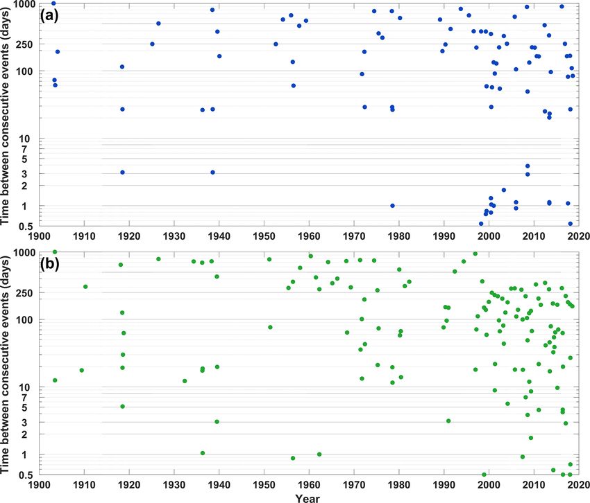
S. A. Stephens et al.: Spatial and temporal analysis                                                                                785

Figure 1. (a) Location of tide gauge sites around NZ, with site number and (b) duration of the sea-level records.

are occasionally recorded too. To enable consistent analysis             like seasonal heating and cooling (Bell and Goring, 1998;
between gauges and within long-duration records with varied              Boon, 2013), and we wished to later analyse seasonal ef-
sampling frequency, we subsampled all sea-level data to 1 h              fects on the timing of extreme storm-tide events. MSLA
intervals after first applying a 15 min running average to min-          was calculated using a 30 d running average of the non-tidal
imize the effect of far infragravity and tsunami waves. Thus,            residual (Haigh et al., 2014) – MSLA is a slowly varying
we analyse still-water levels with short-period wave effects             (≥ 1 month) component of both storm tide and skew surge,
minimized. Some open-coast sites can experience wave set-                which includes seasonal sea-level variability. Skew surge was
up when large waves are present.                                         calculated as the absolute difference between the maximum
   The sea-level heights are specified relative to local verti-          recorded storm tide during each tidal cycle and the predicted
cal datum (Hannah and Bell, 2012). Average relative mean                 maximum astronomical tidal level for that cycle, irrespec-
sea levels in New Zealand have exhibited an approximately                tive of differences in timing between these (Batstone et al.,
linear rise over the last century of 1.7 ± 0.1 mm yr−1 (Han-             2013; Williams et al., 2016) – every high tide has an asso-
nah and Bell, 2012). Therefore, before further analysis the              ciated skew surge. Skew surge is a relevant metric of surge
data were linearly detrended to a zero mean relative to lo-              in tidally dominant locations like NZ (e.g. Merrifield et al.,
cal vertical datum for each gauge, to remove the effects of              2013) because the extreme storm tide and resulting flooding
historical SLR from the sea-level distribution and create a              exposure (excluding wave overtopping) usually occurs for a
quasi-stationary time series required for extreme value anal-            few hours around the high tide.
ysis (Coles, 2001). We used a linear trend rather than remov-               Like Haigh et al. (2016), we investigate two types of
ing annual mean sea level because we wished to retain inter-             events: (1) extreme storm-tide events (relevant to coastal
annual sea-level variability as a long-period component of               flooding) that reached or exceeded the 1 in 5-year return level
MSLA in the storm-tide distribution.                                     (the storm tide equalled or exceeded once, on average, every
   The detrended sea-level records were separated into their             5 years) in the detrended series (i.e. independent of SLR) and
main component parts. Tidal elevations were predicted us-                (2) extreme skew surges that reached or exceeded the 1 in
ing harmonic analysis with 67 constituents following Fore-               5-year return level. Some of the skew-surge events coincide
man et al. (2009), and the tides were subtracted from the                with the extreme storm-tide events, when the storm surge oc-
detrended sea level to obtain the non-tidal residual. The so-            curred around the time of high water of a spring tide; others
lar annual and semi-annual tidal constituents were omitted               do not coincide, because the surge occurred near a small high
from the tidal harmonic predictions because most of the sea-             tide or on a neap tide. In this paper an “event” is defined as
sonal signal is actually driven by non-astronomical effects              a meteorological storm that caused an extreme storm tide or

www.nat-hazards-earth-syst-sci.net/20/783/2020/                                    Nat. Hazards Earth Syst. Sci., 20, 783–796, 2020
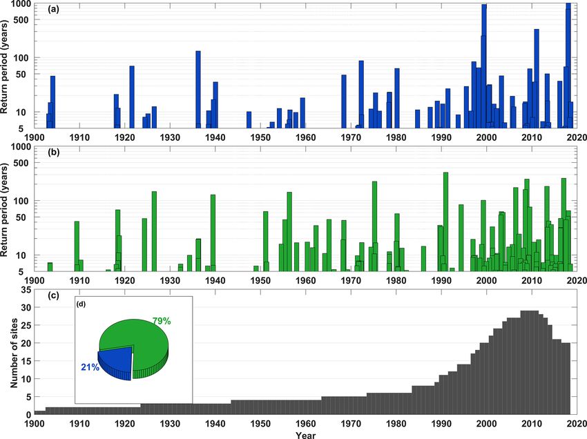
786                                                                        S. A. Stephens et al.: Spatial and temporal analysis

skew surge at least one tide gauge but often at several tide       to identify extreme storm tides and skew surges with ≥ 1 in
gauges – so a single “event” can have multiple observed ex-        5-year return levels for further analysis. We used the SSJPM
tremes.                                                            to determine the return period of extreme storm tides (e.g.
   A generalized Pareto distribution (GPD) fitted to peaks-        Fig. 2a, Supplement Tables S2, S4 and S7) when the GPD
over-threshold (POT) data (Coles, 2001) was used to deter-         and SSJPM methods both indicated a ≥ 10-year return period
mine the 1 in 5-year return level thresholds for identifying       for a particular storm tide, since we prefer the SSJPM method
extreme storm-tide and skew-surge events, because the GPD          but there can be a mismatch between the GPD and SSJPM at
model is fitted directly to the independent storm-tide and         the 5-year return level used for storm-tide maxima selection
skew-surge maxima (e.g. Fig. S1 in the Supplement) asso-           (Fig. S1). Using a SSJPM-based storm-tide threshold would
ciated with storms that we analyse later. POT consisted of         select a slightly different set of storm tides for analysis but
sea-level maxima with the maxima being separated by a min-         would not affect the key results or conclusions.
imum of 3 d, since separate meteorological systems gener-             To characterize storms in the wider NZ region, we used
ally pass over NZ within 4–7 d of each other. A test using         the Kidson (2000) classification of synoptic weather regimes
a 2 d threshold for both storm tide and skew surge showed          associated with clusters of extreme storm tides and/or skew
that the identification of extreme events was insensitive to       surges that impacted at least three tide gauge sites during the
the time threshold. The POT height threshold was selected          event. Kidson (2000) defined three weather “regimes”, char-
to give an average of approximately five high-water maxima         acterized by (i) frequent low-pressure troughs crossing the
per year over the duration of the measurement record, which        country, (ii) high-pressure systems to the north with strong
is equivalent to about the 99.8th percentile of the hourly         zonal flow to the south of the NZ, and (iii) blocking pat-
data (the number of maxima exceeding the height thresh-            terns with high-pressure systems more prominent in the south
old varies year to year). However, for predicting long return-     (Fig. S2). Rueda et al. (2019) used a method of weather typ-
period levels such as for 100 years, the GPD model is likely       ing to develop statistical predictors for storm surge and wave
to be biased low when analysing short sea-level records (e.g.      height in NZ based on statistical relationship with MSL pres-
Fig. S1) due to the likelihood of observing few very large         sure fields. The Kidson (2000) weather regimes are easily as-
maxima over a short record (e.g. I. D. Haigh et al., 2010).        sociated with the extreme storm-tide and skew-surge spatial
Therefore, we also applied the skew-surge joint-probability        clusters identified.
method (SSJPM) (Batstone et al., 2013) to determine ex-
treme storm-tide frequency and magnitude. Joint-probability
methods provide more robust low-frequency magnitude esti-          4     Results
mates for short-duration records because they overcome the
main theoretical limitations of extreme value theory appli-        4.1    Comparison of events
cation to sea levels – splitting the sea level into its deter-
ministic (predictable) tidal and stochastic (e.g. unpredictable,   We compared the dates and return periods for both extreme
storm-driven) non-tidal components, and analysing the two          storm-tide and extreme skew-surge events and ascertained
components separately before recombining (e.g. Tawn and            how many skew-surge events also resulted in extreme storm
Vassie, 1989; I. D. Haigh et al., 2010). Storm-tide return pe-     tides. Extreme storm tides were generated by 85 distinct
riods can be estimated from relatively short records because       storm events (Fig. 2a, Table S2). These 85 storm events con-
all skew surges are considered, not just those that lead to        tributed to 155 independent storm-tide maxima that reached
extreme levels. A limitation of the SSJPM and other joint-         or exceeded the 1 in 5-year return level at any of the 30 sea-
probability methods is that it assumes tide and skew surge         level-gauge sites (Fig. 1) – in other words the storm events
are independent, which has been shown to be true in the UK         sometimes caused extreme storm tides to occur at more than
(Williams et al., 2016) but has not been fully investigated        one sea-level gauge site. In total, 191 skew surges reached
in NZ, although comparisons with direct maxima methods             or exceeded the 1 in 5-year return period across the 30 sites,
for > 50-year-long records (Fig. S1) give similar results for      generated by 135 distinct storm events (Fig. 2b, Table S3).
return periods ≥ 10 years and also match observed maxima           This difference in event numbers is consistent with NZ’s
well, and thus support the validity of the independence as-        coastal context of meso- to micro-tidal ranges and moderate
sumption for long-return-period events. Santamaria-Aguilar         storm surges, which are usually several decimetres (not me-
and Vafeidis (2018) found skew surge to be independent of          tres) high, meaning tides are a key determinant (or precursor)
high-tide height in mixed semi-diurnal tidal regimes located       for coastal flooding rather than solely storm surges.
in regions with a narrow continental shelf, like NZ. How-             Like Haigh et al. (2016), there are unavoidable issues with
ever, this may not be the case inside harbours where storm         the database that arise because hourly tide gauge records do
surge magnitude can depend on the tidal stage (e.g. Bernier        not cover all the full 118-year period analysed since the start
and Thompson 2007; Horsburgh and Wilson, 2007; Goring              of the Auckland and Dunedin records in 1900. It is obvious,
et al., 2011). In summary, the GPD/POT model was used to           examining Fig. 2c, that we are likely missing many events
determine extreme skew-surge frequency and magnitude and           before the early 1990s, when records were spatially sparse.

Nat. Hazards Earth Syst. Sci., 20, 783–796, 2020                             www.nat-hazards-earth-syst-sci.net/20/783/2020/
S. A. Stephens et al.: Spatial and temporal analysis                                                                                    787

Figure 2. (a) Return period of the highest storm tides in each of the 85 extreme storm-tide events (resulting in 155 extreme storm-tide
observations), offset for mean sea level; (b) return period of the highest skew surges in each of the 135 skew-surge events (resulting in 191
extreme skew-surge observations); (c) the number of sites per annum for which sea-level data are available across the 30 sites; and (d) pie
chart showing the number of skew-surge events that led to extreme storm-tide events (blue) and the number that did not (green).

The decline in data availability post-2010 occurs due to dis-            with astronomical spring high tides. Occasionally a smaller
continuation of some sea-level gauges around that time, but              high tide combined with a large skew surge to produce an ex-
there are also some recent records that we were unable to                treme storm tide – more so for sites with a micro-tidal range
obtain for analysis. The highest return period from two no-              (e.g. Wellington; see Fig. 3). The ratio of maximum observed
table historical storms is probably lower than it should be,             skew surge to maximum observed storm tide ranged from
e.g. the great 1936 ex-tropical cyclone (Brenstrum, 2000)                0.23 to 0.51 with a median of 0.34 (Fig. S3). The tide is usu-
and ex-tropical cyclone Giselle in 1968 (Revell and Gorman,              ally the dominant component of sea-level height, even during
2003). Although we have data at some sites for these events,             extreme events, and extreme storm tides occur close to high
tide gauges were not necessarily operational at the time along           tide and are unlikely during a small neap high tide. Extreme
the stretches of the coastline where the storm tides or skew             storm-tide elevation is linearly related to mean high water
surges were likely to have been most extreme; this is the case           spring (MHWS) elevation (Fig. 4). Equations 1 and 2 are
for the 1936 (except in Auckland) and 1968 events. Notwith-              the least-squares linear fits between the MHWS-7 (the height
standing these issues, our analysis of the events that we have           equalled or exceeded by the highest 7 % of all high tides)
on record does provide important insights, as described be-              and the 5-year and 100-year return storm tide, respectively.
low.                                                                     Outliers to the linear fits occur in some upper-estuarine loca-
   It is not possible for tide alone to result in a ≥ 1 in 5-            tions where the skew-surge / storm-tide ratios are relatively
year return period extreme storm tide, so all observed storm             large (Fig. S3).
tides were associated with storms that produced skew surge.
However, only 29 of the 135 (21 %) extreme skew-surge
events led to extreme storm tides (Fig. 2d), while the ma-               5-year return period extreme storm tide (m)
jority (79 %) did not. Hence, as Haigh et al. (2016) found for           = 1.20 × MHWS-7 + 0.23                                          (1)
the UK coast, most extreme storm tides arose from moderate               100-year return period extreme storm tide (m)
(i.e. < 1 in 5-year return levels) skew-surge events combined
                                                                         = 1.32 × MHWS-7 + 0.28                                          (2)

www.nat-hazards-earth-syst-sci.net/20/783/2020/                                    Nat. Hazards Earth Syst. Sci., 20, 783–796, 2020
788 S. A. Stephens et al.: Spatial and temporal analysis
Figure 3. The contributions of tide, skew surge and MSLA to the ≥ 1 in 5-year return period extreme storm-tide maxima at two of NZ’s
longest sea-level recorders with a meso-tidal (a Auckland) and micro-tidal (b Wellington) range. HAT denotes the highest astronomical tide,
MHWS-7 is the height equalled or exceeded by the highest 7 % of all high tides, MinHW denotes lowest high tide height; SS5year is the
height of the 1 in 5-year return period skew surge.
During the highest extreme storm tides, all sea-level com- footprints were most commonly associated with block-
ponents tended to be large and positive (Fig. S4), with the ing weather types (Fig. 5), low-pressure systems that
tide being the largest component, but skew surge and MSLA tracked from north of NZ (Fig. 6) and intensified next to
being relatively larger in the highest storm tides (Fig. S5). a blocking high-pressure system lying east of NZ. Cat-
The MSLA was positive in 92 % of all extreme storm tides egory 1 footprints had storm centres that lay over the
and in 88 % of all extreme skew surges. North Island or north of NZ at the time of maximum
storm tide or skew surge, with a mean position located
4.2 Spatial analysis just off the northeast coast of the North Island (Fig. 6).
We then considered the spatial characteristics of events 2. Category 2 footprints impacted everywhere but mainly
around the coast. As expected, and as Haigh et al. (2016) the South Island (Fig. 1a) and the west coast of the
noted for the UK, there is a significant (95 % confidence North Island (Fig. 5). Category 2 footprints were gen-
level) correlation (0.50 for the storm-tide events and 0.47 erally associated with trough weather regimes, which
for the skew-surge events) between the highest return period were the most common event drivers. Troughs were
of the events and the number of tide gauge sites impacted associated with storm centres that tracked eastwards
(Fig. S6). across NZ, usually across or south of the South Island
To investigate the different spatial extents of coastline af- and always south of the northernmost tip of NZ (Fig. 6).
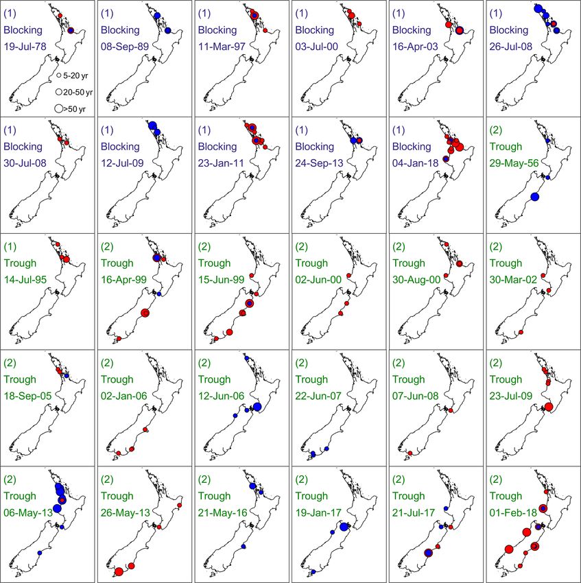
fected, we identified 30 storm events that impacted three or Category 2 footprints had storm centres at the time of
more gauge sites concurrently (Fig. 5). We observed two sep- maximum storm tide that lay in an arc across the South
arate categories of spatial footprints, which can be related to Island from northwest to southeast, with a mean posi-
the Kidson (2000) weather regimes (Fig. S2) as follows: tion located southeast of the South Island (Fig. 6).
1. Category 1 footprints predominantly impacted the The largest events with return periods ≥ 1 in 50 years were
northeast coast of the North Island and occasionally the more common on the east coast of the North Island during
west coast of the North Island (see Fig. 1a). Category 1 blocking weather types, whereas trough weather types were
Nat. Hazards Earth Syst. Sci., 20, 783–796, 2020 www.nat-hazards-earth-syst-sci.net/20/783/2020/S. A. Stephens et al.: Spatial and temporal analysis 789
Figure 4. Linear relationship between high tide and storm tide in NZ. MHWS-7 is the height equalled or exceeded by the highest 7 % of all
high tides. RP denotes return period, also known as average recurrence interval.
more common in the South Island and along the west coast ing of extreme storm tide is perhaps surprising given the
of the North Island (Fig. 5). dominance of tide on the storm-tide elevation (Figs. 3 and 4).
But because two spring tidal cycles per month provide suffi-
4.3 Temporal analysis cient monthly “exposure potential” for storm-tide events, the
seasonal pattern is then strongly influenced by the mean an-
Next, we examined the temporal variation in events. Ex- nual MSLA cycle. Once the effect of the mean annual MSLA
treme storm-tide events with ≥ 1 in 5-year return level occur cycle is removed, the seasonal distributions of both extreme
throughout the year but are least frequent in late winter and storm-tide and skew-surge events are more uniform through-
early spring (September–December) (Fig. 7). Extreme storm- out the year (Figs. S8 and S9), although there is still a ten-
tide events with ≥ 1 in 25-year return level exhibit a peak in dency for a lower number of extreme storm-tide and skew-
January that tapers off through to May followed by another surge events near the end of the year in October–December.
peak in June that tapers off through to September. No storm- In terms of inter-annual climate effects on extreme storm
tide events with ≥ 1 in 25-year return level were observed in tides, we found no relationship between extreme storm-tide
September–December. Like extreme storm tide, skew surges height or return period and large-scale climate modes, such
with ≥ 1 in 5-year return level are also least likely in the lat- as the El Niño–Southern Oscillation (ENSO) and Southern
ter half of the year and were most frequent March–July. Annular Mode (SAM; e.g. Fig. S10, Table S10 Trenberth,
The largest tidal constituents around NZ are the M2, S2 1976). This aligns with the findings of Lorrey et al. (2014)
and N2 semi-diurnal constituents. The seasonal pattern in the that ex-tropical cyclone tracks and locations relative to Auck-
height of the highest tides, which peak around March and land at their point of closest passage are not directly linked
September (Fig. 7d), is affected by the solar equinox. How- to the phase of ENSO or SAM, but they are linked more
ever, the seasonal pattern in the number of extreme storm- closely to atmospheric circulation conditions that develop
tide and skew-surge events does not follow the highest tides in the southwestern Pacific, to the north of and over New
but appears to follow the seasonal pattern of MSLA – MSLA Zealand. In other words, extreme storm-tide events are in-
being a component of both extreme storm-tide and skew- fluenced by random weather events rather than large-scale
surge elevations. The mean annual MSLA cycle is domi- climate variability modes.
nated by thermo-steric sea-level adjustments and secondary- Following Haigh et al. (2016), we examined temporal clus-
forcing variables of barometric pressure and alongshore wind tering by considering the number of days between consecu-
stress (Bell and Goring, 1998), and it peaks between March tive events. There are no instances of storm-tide events hap-
and June in NZ – at 22 of 30 sites it peaks in May due pening within 4–10 d of each other, whereas there are occa-
to the thermosteric lag. The range of the 95 % confidence sions when pairs of skew-surge events occurred within that
intervals of the annual sea-level cycle was about −0.15 to time interval (Fig. 8). Only once did two extreme storm-tide
+0.15 m around NZ, and the median amplitude across all events occur within < 4 d of each other, when two separate
sites was 0.04 m (Fig. S7). Yet MSLA can be larger in any low-pressure systems intensified against a blocking high-
single month and tended to be larger during observed ex- pressure system and impacted NZ on 27 and 30 July 2008.
treme events – MSLA during events ranged from −0.06 to
0.28 m (Tables S2 and S3). The MSLA influence on the tim-
www.nat-hazards-earth-syst-sci.net/20/783/2020/ Nat. Hazards Earth Syst. Sci., 20, 783–796, 2020790 S. A. Stephens et al.: Spatial and temporal analysis
Figure 5. The spatial footprints of all the storm-tide or skew-surge events that impacted at least three tide gauge sites. Red circle denotes
extreme storm tide; blue circle denotes extreme skew surge. Circle diameter matched to return periods of 5–20, 20–50 and ≥ 50 years (small
to large respectively). The spatial cluster category (1 or 2), Kidson weather type and date during each event are shown.
5 Discussion of Water and Atmospheric Research; https://niwa.co.nz/
our-science/coasts/tools-and-resources/tide-resources, last
5.1 Tidal influence access: 10 March 2020). The red-alert tide concept works
in New Zealand because the semi-diurnal tides dominate
In NZ, we find that most of the extreme storm tides are sea-level variability and storm surges are limited to mostly
driven by moderate skew surges combined with high spring < 0.5 m, which is approximately 25 % of the average tidal
or perigean spring tides, which is similar to the UK despite range (Stephens et al., 2014). Coastal or hazard managers
the fact that the UK has larger tides and a slightly smaller are advised to keep a close watch on the weather for lower
surge / tide ratio (Figs. S3c and S10c of Haigh et al., 2016) barometric pressure and adverse winds during the red-alert
and is also similar for annual maxima around much of tide days, as even a minor storm or swell event could lead
the world (Merrifield et al., 2013). We found that extreme to inundation of low-lying areas, especially if accompanied
storm-tide elevations are strongly correlated with MHWS by waves (Bell, 2010). In practice, weather forecasts alert
elevation. This affirms current practice in NZ of forecasting managers to high surges and storm tides with < 10 d notice,
“red-alert” tide dates when high-tide peaks are predicted but the red-alert tide calendars enable resource planning (e.g.
to be unusually high (Bell, 2010; Stephens et al., 2014) staff leave days) months in advance of potential high-storm-
(see NZ Storm-Tide Red-Alert Days; National Institute tide days and are a valued coastal climate service in NZ. For
Nat. Hazards Earth Syst. Sci., 20, 783–796, 2020 www.nat-hazards-earth-syst-sci.net/20/783/2020/S. A. Stephens et al.: Spatial and temporal analysis 791
Figure 6. Storm tracks and weather types contributing to all the storm-tide or skew-surge events that impacted at least three tide gauge sites.
Storm tracks and the location of the storm centre at storm-tide event peak are marked for both blocking (green and blue) and trough (red and
brown) Kidson (2000) weather types. Open circles denote storm track origin.
example, the highest storm tide in Auckland (NZ) on record
since 1900 occurred on 23 January 2011, closing major city
highways, and causing millions of dollars of flood-related
damage. At 0.52 m the skew surge was relatively large
for NZ and coincided with a predicted “red alert” (high
perigean spring) tide, and a background MSLA of nearly
0.05 m, noting that ongoing SLR increasingly adds to the
impact or frequency of flooding (Stephens et al., 2018). SLR
of about 0.12 m between 1936 and 2011 means that after
detrending for sea-level rise the 2011 storm tide is actually
the second-largest storm tide with the 26 March 1936 storm
tide being largest (Fig. 3a).
The observed linear relationships between extreme storm
tide and MHWS elevation have proven useful for esti-
mation of extreme storm tide at locations without long-
term sea-level gauges – extreme storm tide can be pre-
dicted using short-term sea-level recorder deployments to
establish tidal elevations, or a tidal model (e.g. see New
Zealand Tide Forecaster; https://niwa.co.nz/our-science/
coasts/tools-and-resources/tide-resources). However, rela-
tively large extreme storm tide in some upper-estuarine lo-
cations plotted as outliers to the linear relationships (Figs. 4,
Figure 7. Seasonal distribution of sea-level components associated S3). Research has shown that non-linear interactions between
with extreme storm-tide and skew-surge events: (a) extreme storm tide, wind and morphology influence surge generation inside
tide, (b) extreme skew surge, (c) MSLA and (d) high tide ≥ 93rd enclosed estuaries (e.g. Plüß et al., 2001; Rego and Li, 2010;
percentile (includes all high tides, not just those associated with ex-
Orton et al., 2012), a subject for further research in NZ since
treme storm-tide events). N denotes number of occasions.
there are few long-term sea-level records to help quantify
www.nat-hazards-earth-syst-sci.net/20/783/2020/ Nat. Hazards Earth Syst. Sci., 20, 783–796, 2020792 S. A. Stephens et al.: Spatial and temporal analysis
Figure 8. Time between successive events: (a) storm tide and (b) skew surge.
extreme storm-tide frequency and magnitude in NZ upper- lier emergence of flooding due to greater sensitivity to SLR
estuarine locations. (Hunter, 2012).
5.3 Surge influence
5.2 MSLA influence
NZ is similar to the UK in that temporal clustering of storm-
The median amplitude of the mean annual sea-level cycle tide events is controlled by the spring tide cycle (Haigh et
from all sea-level records is only 0.04 m, yet the annual al., 2016), with storm-tide events generally not occurring
MSLA cycle is a strong influence on the monthly timing within 10 d of each other historically. However, it only re-
of extreme storm-tide and skew-surge events. MSLA was quires storm surge to elevate high tides to an extreme storm-
positive in 92 % of all sea level and in 88 % of all extreme tide level. Therefore, extreme storm tides and skew surges
skew-surge events and is clearly an influential component of do not strike NZ-wide but exhibit spatial clustering associ-
the highest storm tides (Figs. S3–S4, S7–S8). The sensitiv- ated with storm tracks that have general patterns related to
ity of extreme storm tide to relatively small MSLA shows weather types.
that small increases in mean sea level, from long-term SLR, During the spring and summer of 2017 and 2018 several
will cause a large increase in the frequency of extreme storm large storms including ex-tropical cyclones Fehi, Gita and
tide, a result consistent with other studies (e.g. Hunter, 2012; Hola struck NZ, most of them coinciding with high perigean
Sweet and Park, 2014; Stephens et al., 2018). Tidally domi- spring tides, causing flooding to homes and damaging in-
nated sites like NZ, where the tide is the key determinant of frastructure. Other notable historical coastal flooding events
extreme storm tide, will be more sensitive to SLR in terms of in NZ occurred in January 2011, during cyclone Giselle in
the increasing frequency of extreme storm-tide events than 1968 (de Lange and Gibb, 2000), May 1938 in the Hauraki
surge-dominated sites (Vitousek et al., 2017; Rueda et al., Plains (Stephens, 2018) and during the great cyclone of 1936
2017; Stephens et al., 2018). This is because tidally dom- (Brenstrum, 2000), but the spatial effects of these historical
inated sites have a relatively flat upper tail on the extreme storms are not well recorded since many sea-level gauges
storm-tide frequency–magnitude distribution. Many parts of were not operating at those times (Fig. 1). The calculated ex-
the world are even more tidally dominant than NZ (Merri- treme storm-tide and skew-surge frequency and magnitudes
field et al., 2013; Rueda et al., 2017) and will experience ear- (Tables S7 and S8) are based on available digital records but
Nat. Hazards Earth Syst. Sci., 20, 783–796, 2020 www.nat-hazards-earth-syst-sci.net/20/783/2020/S. A. Stephens et al.: Spatial and temporal analysis 793
could be biased low in places where historical storms are not We analysed extreme storm tide and skew surge for 30
included. A notable example is in Tauranga Harbour, where sea-level records of varying length throughout NZ. Numer-
the highest skew surge ever recorded in NZ by a sea-level ical models, properly calibrated, provide a means of extend-
gauge occurred during cyclone Giselle in 1968 and reached ing the extreme storm-tide analyses to develop probabilis-
0.88 m above the predicted high tide (de Lange and Gibb, tic assessments of total water level along the entire coast-
2000). However, that tide gauge is no longer operating and line. These can include combinations of tidal (e.g. Walters et
hourly data were not available for inclusion in this analy- al., 2001), storm-surge and wave models (e.g. Gorman et al.,
sis. We applied a joint-probability method to determine the 2003; Rueda et al., 2019), which can include both hindcasts
frequency–magnitude distribution of extreme storm tide (Ta- and climate-change future casts (Cagigal et al., 2019). How-
ble S7), which partially overcomes the limitation of short- ever, numerical storm-surge models for climate change typ-
duration sea-level records. ically do not include MSLA, which is an important compo-
Before the analysis presented here, the largest recorded nent of extreme storm tide (for tidally dominant coasts) and
skew surge was 0.88 m measured in Tauranga Harbour in hence flooding exposure (e.g. Stephens et al., 2014; Sweet
1968. We observed 15 larger skew surges at enclosed estu- and Park, 2014), and which we have shown to be an im-
arine sites (Fig. 1a): 1 at Helensville (site 29), 1 at Raglan portant influence on the timing of extreme events. Efforts to
(site 26), 2 at Kawhia (site 25) and 11 at Invercargill (site forecast MSLA are being made (Widlansky et al., 2017), but
18). The maximum skew surge from our analysis was 1.15 m work is required to include MSLA into models for the devel-
at Raglan on 6 May 2013, and a skew surge of 1.26 m was opment of probabilistic assessment of extreme water levels
inferred from anecdotal evidence in the northern Hauraki to assess coastal hazard risks, taking into account SLR.
Plains on 4 May 1938 (Table S2, Stephens, 2018). However,
a much larger non-tidal residual sea level (NTR) was mea-
sured at the open-coast Jackson Bay site around low tide, dur- 6 Conclusions
ing ex-tropical cyclone Fehi on 1 February 2018 (Fig. S12).
In this paper we analysed sea-level records to quantify ex-
NTR is the difference between the measured storm tide and
treme storm-tide and skew-surge frequency and magnitude
the predicted tide and is calculated over the full tidal cycle
around the coast of NZ for the first time. We identified the
at the sampling frequency of the sea-level record, hourly in
relative magnitude of sea-level components contributing to
this case. The NTR at Jackson Bay on 1 February 2018 ap-
85 extreme storm-tide and 135 extreme skew-surge events
peared to be a meteorologically forced wave that peaked at
(≥ 5-year return period), which have been recorded in NZ
2.29 m near low tide (Fig. S12) and would have created a
since 1900. We examined spatial and temporal clustering of
much higher storm tide if it had peaked at high tide – the
extreme storm-tide and skew-surge events and identified typ-
skew surge was 0.69 m. Although this was the highest storm
ical storm-tracks and weather types in the SW Pacific asso-
tide on record at Jackson Bay, it was a near miss to a much
ciated with spatial clusters of extreme sea levels.
higher storm tide. We found that the “potential” storm tide,
We found that around NZ most extreme storm tides
constructed from the sum of the maximum observed tide and
are driven by moderate skew surges combined with high
skew surge, was 7 %–20 % higher than the estimated 100-
perigean spring tides. Extreme storm-tide elevations are
year return period extreme storm-tide level (Table S9). Hence
highly correlated with and linearly related to mean spring
the potential exists for higher and more damaging storm tides
high-tide elevation, enabling prediction of extreme storm-
than historically observed in the patchy NZ records, even
tide elevations in ungauged areas from tidal information,
without considering the effects of future SLR. Alongside the
which is readily available from short-term measurements or
provided frequency–magnitude estimates, it would be sensi-
tidal models.
ble to consider these “potential” extreme storm-tide eleva-
The spring–neap tidal cycle, coupled with a small to mod-
tions when planning or managing low-lying coastal land use.
erate skew-surge climatology, prevents successive extreme
We analysed still-water levels with wave effects removed
storm-tide events from happening within 4–10 d of each
from the record (apart from wave set-up that may be im-
other. Of 85 extreme storm-tide events, only once did two ex-
plicit in measurements for some events at open-coast gauges,
treme storm tides occur less than 4 d apart due to two closely
e.g. site 8). Waves are often present during storms, and wave
spaced storms straddling a peak spring tide period. Generally,
set-up and run-up can raise the water level at the coast sub-
there are at least 10 d between extreme storm-tide events.
stantially, especially on steeper beach gradients or steep-face
structures such as rock revetments or seawalls (e.g. Stockdon
et al., 2006; Stephens et al., 2011). Hazard analyses should
account for wave effects, including far infragravity surges,
in wave-exposed locations, on top of the extreme storm tide
presented here. An analysis of the spatial and temporal clus-
tering of extreme wave events could also be undertaken, fol-
lowing the approach of Santos et al. (2017).
www.nat-hazards-earth-syst-sci.net/20/783/2020/ Nat. Hazards Earth Syst. Sci., 20, 783–796, 2020794 S. A. Stephens et al.: Spatial and temporal analysis
Extreme events caused by “blocking” weather types co- Financial support. This research has been supported by the New
incided with storm centres located in the north of NZ and Zealand Ministry of Business, Innovation and Employment (Strate-
predominantly impacted the northeast coast and occasionally gic Science Investment Fund projects CAVA1904 and CARH2002
the west coast of the North Island. Extreme events caused – National Institute of Water and Atmospheric Research).
by “trough” weather types coincided with storm centres that
track further south, across or south of NZ and impacted
mainly the South Island and the west coast of the North Is- Review statement. This paper was edited by Thomas Wahl and re-
viewed by Franck Mazas and one anonymous referee.
land.
Lower numbers of extreme storm-tide and skew-surge
events were observed in late spring to early summer (which
is also outside the ex-tropical cyclone season). This reflects a References
tendency for more extreme surges earlier in the year but was
also noticeably influenced by the mean annual sea-level cy- Batstone, C., Lawless, M., Tawn, J., Horsburgh, K., Blackman, D.,
cle that peaks in the austral autumn in most places. There is McMillan, A., Worth, D., Laeger, S., and Hunt, T.: A UK best-
no apparent relationship between extreme storm-tide events practice approach for extreme sea-level analysis along complex
topographic coastlines, Ocean Eng., 71, 28–39, 2013.
and large-scale climate-variability modes such as ENSO. The
Bell, R. G.: Tidal exceedances, storm tides and the effect of sea-
considerable influence of the relatively low-amplitude mean level rise, Proceedings of the 17th Congress of the Asia and Pa-
sea-level anomaly shows that a relatively small SLR will cific division of the IAHR, Auckland, New Zealand, 10, 2010.
drive rapid increases in the frequency of presently rare ex- Bell, R. G. and Goring, D. G.: Seasonal variability of sea level and
treme storm tides. sea-surface temperature on the north-east coast of New Zealand,
Estuar. Coast. Shelf S., 47, 307–318, 1998.
Bernier, N. B. and Thompson, K. R.: Predicting the frequency of
Data availability. Some of the sea-level records used for the work storm surges and extreme sea levels in the northwest Atlantic, J.
are available from the Global Sea Level Observing System website Geophys. Res.-Oceans, 111, 10009–10009, 2006.
run by the University of Hawaii Sea Level Center. Other records are Bernier, N. B. and Thompson, K. R.: Tide-surge interaction off the
privately owned and are available from NZ port companies by direct east coast of Canada and northeastern United States, J. Geophys.
request. Extreme storm-tide and skew-surge data (for reproduction Res.-Oceans, 112, 6008–6008, 2007.
of plots within the manuscript) are included in the supplementary Boon, J. D.: Secrets of the tide: tide and tidal current analysis
tables. and predictions, storm surges and sea level trends, Elsevier,
https://doi.org/10.1016/C2013-0-18114-7, 2013.
Brenstrum, E.: The cyclone of 1936: the most destructive storm of
Supplement. The supplement related to this article is available on- the Twentieth Century?, Weather and Climate, 20, 23–27, 2000.
line at: https://doi.org/10.5194/nhess-20-783-2020-supplement. Cagigal, L., Rueda, A., Castanedo, S., Cid, A., Perez, J., Stephens,
S. A., Coco, G., and Méndez, F. J.: Historical and future
storm surge around New Zealand: From the 19th century to
Author contributions. SAS designed the concept with input from the end of the 21st century, Int. J. Climatol., 40, 1512–1525,
RGB and IH. IH provided Matlab code. SAS undertook the analyses https://doi.org/10.1002/joc.6283, 2020.
and wrote the paper, with input from RGB and IH. RGB examined Coles, S.: An introduction to statistical modeling of extreme values,
the relationship between sea level and large-scale climate modes. Springer, London, New York, 2001.
de Lange, W. P. and Gibb, J. G.: Seasonal, interannual, and decadal
variability of storm surges at Tauranga, New Zealand, New Zeal.
J. Mar. Fresh., 34, 419–434, 2000.
Competing interests. The authors declare that they have no conflict
Foreman, M. G. G., Cherniawsky, J. Y., and Ballantyne, V. A.: Ver-
of interest.
satile Harmonic Tidal Analysis: Improvements and Applications,
J. Atmos. Ocean. Tech., 26, 806–817, 2009.
Goring, D. G. and Bell, R. G.: El Nino and decadal effects on sea-
Special issue statement. This article is part of the special issue “Ad- level variability in northern New Zealand: a wavelet analysis,
vances in extreme value analysis and application to natural haz- New Zeal. J. Mar. Fresh., 33, 587–598, 1999.
ards”. It is not associated with a conference. Goring, D. G., Stephens, S. A., Bell, R. G., and Pearson, C. P.: Esti-
mation of Extreme Sea Levels in a Tide-Dominated Environment
Using Short Data Records, J. Waterw. Port C., 137, 150–159,
Acknowledgements. Benjamin Robinson processed sea-level data. 2011.
Sea-level data were obtained from NIWA and from various port Gorman, R. M., Bryan, K. R., and Laing, A. K.: Wave hindcast for
companies and regional councils in New Zealand. Ron Oven- the New Zealand region: nearshore validation and coastal wave
den pre-reviewed the manuscript. Thanks to Franck Mazas and climate, New Zeal. J. Mar. Fresh., 37, 567–588, 2003.
an anonymous reviewer whose review helped to improve the Haigh, I., Nicholls, R., and Wells, N.: Assessing changes in extreme
manuscript. sea levels: Application to the English Channel, 1900–2006, Cont.
Shelf Res., 30, 1042–1055, 2010.
Nat. Hazards Earth Syst. Sci., 20, 783–796, 2020 www.nat-hazards-earth-syst-sci.net/20/783/2020/S. A. Stephens et al.: Spatial and temporal analysis 795 Haigh, I. D., Nicholls, R., and Wells, N.: A comparison of the main York City region, J. Geophys. Res.-Oceans, 117, C09030, methods for estimating probabilities of extreme still water levels, https://doi.org/10.1029/2012jc008220, 2012. Coast. Eng., 57, 838–849, 2010. Paulik, R., Stephens, S. A., Wadhwa, S., Bell, R., Popovich, B., Haigh, I. D., Wijeratne, E. M. S., MacPherson, L. R., Pattiaratchi, and Robinson, B.: Coastal Flooding Exposure Under Future Sea- C. B., Mason, M. S., Crompton, R. P., and George, S.: Estimating level Rise for New Zealand. NIWA Client Report 2019119WN, present day extreme water level exceedance probabilities around prepared for The Deep South Science Challenge, March 2019, the coastline of Australia: tides, extra-tropical storm surges and 76 pp., 2019. mean sea level, Clim. Dynam., 42, 121–138, 2014. Paulik, R., Stephens, S. A., Bell, R. G., Wadhwa, S., and Popovich, Haigh, I. D., Wadey, M. P., Wahl, T., Ozsoy, O., Nicholls, R. B.: National-Scale Built-Environment Exposure to 100-Year Ex- J., Brown, J. M., Horsburgh, K., and Gouldby, B.: Spatial and treme Sea Levels and Sea-Level Rise, Sustainability, 12, 1513, temporal analysis of extreme sea level and storm surge events https://doi.org/10.3390/su12041513, 2020. around the coastline of the UK, Scientific Data, 3, 160107, Plüß, A., Rudolph, E., and Schrodter, D.: Characteristics of storm https://doi.org/10.1038/sdata.2016.107, 2016. surges in German estuaries, Clim. Res., 18, 71–76, 2001. Hannah, J. and Bell, R. G.: Regional sea level trends in Rego, J. L. and Li, C.: Storm surge propagation in Galveston Bay New Zealand, J. Geophys. Res.-Oceans, 117, C01004, during Hurricane Ike, J. Marine Syst., 82, 265–279, 2010. https://doi.org/10.1029/2011JC007591, 2012. Revell, M. J. and Gorman, R. M.: The “Wahine storm”: evaluation Hinkel, J., Lincke, D., Vafeidis, A. T., Perrette, M., Nicholls, R. J., of a numerical forecast of a severe wind and wave event for the Tol, R. S. J., Marzeion, B., Fettweis, X., Ionescu, C., and Lever- New Zealand coast, New Zeal. J. Mar. Fresh., 37, 251–266, 2003. mann, A.: Coastal flood damage and adaptation costs under 21st Rueda, A., Vitousek, S., Camus, P., Tomás, A., Espejo, A., Losada, century sea-level rise, P. Natl. Acad. Sci. USA, 111, 3292–3297, I. J., Barnard, P. L., Erikson, L. H., Ruggiero, P., Reguero, B. G., 2014. and Mendez, F. J.: A global classification of coastal flood hazard Horsburgh, K. J. and Wilson, C.: Tide-surge interaction and its role climates associated with large-scale oceanographic forcing, Sci. in the distribution of surge residuals in the North Sea, J. Geophys. Rep.-UK, 7, 5038, https://doi.org/10.1038/s41598-017-05090-w, Res.-Oceans, 112, 8003–8003, 2007. 2017. Hunter, J.: A simple technique for estimating an allowance for un- Rueda, A., Cagigal, L., Antolínez, J. A. A., Albuquerque, J. C., Cas- certain sea-level rise, Climatic Change, 113, 239–252, 2012. tanedo, S., Coco, G., and Méndez, F. J.: Marine climate variabil- Jongman, B., Ward, P. J., and Aerts, J. C. J. H.: Global exposure to ity based on weather patterns for a complicated island setting: river and coastal flooding: Long term trends and changes, Global The New Zealand case, Int. J. Climatol., 39, 1777–1786, 2019. Environ. Chang., 22, 823–835, 2012. Santamaria-Aguilar, S. and Vafeidis, A. T.: Are Extreme Skew Kidson, J. W.: An analysis of New Zealand synoptic types and their Surges Independent of High Water Levels in a Mixed Semidi- use in defining weather regimes, Int. J. Climatol., 20, 299–316, urnal Tidal Regime?, J. Geophys. Res.-Oceans, 123, 8877–8886, 2000. 2018. Lagmay, A. M. F., Agaton, R. P., Bahala, M. A. C., Briones, J. B. L. Santos, V. M., Haigh, I. D., and Wahl, T.: Spatial and Temporal T., Cabacaba, K. M. C., Caro, C. V. C., Dasallas, L. L., Gonzalo, Clustering Analysis of Extreme Wave Events around the UK L. A. L., Ladiero, C. N., Lapidez, J. P., Mungcal, M. T. F., Puno, Coastline, Journal of Marine Science and Engineering, 5, 28, J. V. R., Ramos, M. M. A. C., Santiago, J., Suarez, J. K., and https://doi.org/10.3390/jmse5030028, 2017. Tablazon, J. P.: Devastating storm surges of Typhoon Haiyan, Int. Stephens, S. A.: Storm-tide analysis of Tararu sea-level record, J. Disast. Risk Re., 11, 1–12, 2015. NIWA Client Report 2018289HN for Waikato Regional Coun- Lorrey, A. M., Griffiths, G., Fauchereau, N., Diamond, H. J., Chap- cil, October 2018, 34 pp., 2018. pell, P. R., and Renwick, J.: An ex- tropical cyclone climatology Stephens, S. A., Coco, G., and Bryan, K. R.: Numerical simulations for Auckland, New Zealand, Int. J. Climatol., 34, 1157–1168, of wave setup over barred beach profiles: implications for pre- 2014. dictability, J. Waterw. Port C.-ASCE, 137, 175–181, 2011. Menéndez, M. and Woodworth, P. L.: Changes in ex- Stephens, S. A., Bell, R. G., Ramsay, D., and Goodhue, N.: High- treme high water levels based on a quasi-global tide- Water Alerts from Coinciding High Astronomical Tide and High gauge data set, J. Geophys. Res.-Oceans, 115, C10011, Mean Sea Level Anomaly in the Pacific Islands Region, J. At- https://doi.org/10.1029/2009JC005997, 2010. mos. Ocean. Tech., 31, 2829–2843, 2014. Merrifield, M. A., Genz, A. S., Kontoes, C. P., and Marra, J. J.: Stephens, S. A., Bell, R. G., and Lawrence, J.: Developing signals Annual maximum water levels from tide gauges: Contributing to trigger adaptation to sea-level rise, Environ. Res. Lett., 13, factors and geographic patterns, J. Geophys. Res.-Oceans, 118, 104004, https://doi.org/10.1088/1748-9326/aadf96, 2018. 2535–2546, 2013. Stockdon, H. F., Holman, R. A., Howd, P. A., and Sallenger, A. H.: Muis, S., Verlaan, M., Winsemius, H. C., Aerts, J. C. Empirical parameterization of setup, swash, and runup, Coast. J. H., and Ward, P. J.: A global reanalysis of storm Eng., 53, 573–588, 2006. surges and extreme sea levels, Nat. Commun., 7, 11969, Sweet, W. V. and Park, J.: From the extreme to the mean: Accelera- https://doi.org/10.1038/ncomms11969, 2016. tion and tipping points of coastal inundation from sea level rise, Needham, H. F., Keim, B. D., and Sathiaraj, D.: A review of trop- Earths Future, 2, 579–600, 2014. ical cyclone-generated storm surges: Global data sources, obser- Tawn, J. A. and Vassie, J. M.: Extreme sea-levels: the joint proba- vations, and impacts, Rev. Geophys., 53, 545–591, 2015. bilities method revisited and revised, Proceedings of the Institute Orton, P., Georgas, N., Blumberg, A., and Pullen, J.: Detailed of Civil Engineering Part 2, 87, 429–442, 1989. modeling of recent severe storm tides in estuaries of the New www.nat-hazards-earth-syst-sci.net/20/783/2020/ Nat. Hazards Earth Syst. Sci., 20, 783–796, 2020
796                                                                           S. A. Stephens et al.: Spatial and temporal analysis

Thiebaut, S., McComb, P., and Vennell, R.: Prediction of Coastal       Walters, R. A., Goring, D. G., and Bell, R. G.: Ocean tides around
   Far Infragravity Waves from Sea-Swell Spectra, J. Waterw. Port        New Zealand, New Zeal. J. Mar. Fresh., 35, 567–579, 2001.
   Coast., 139, 34–44, 2013.                                           Widlansky, M. J., Marra, J. J., Chowdhury, M. R., Stephens, S. A.,
Trenberth, K. E.: Fluctuations and trends in indices of the south-       Miles, E. R., Fauchereau, N., Spillman, C. M., Smith, G., Beard,
   ern hemispheric circulation, Q. J. Roy. Meteor. Soc., 102, 65–75,     G., and Wells, J.: Multimodel Ensemble Sea Level Forecasts for
   1976.                                                                 Tropical Pacific Islands, J. Appl. Meteorol. Clim., 56, 849–862,
Vitousek, S., Barnard, P. L., Fletcher, C. H., Frazer, N., Erikson,      2017.
   L., and Storlazzi, C. D.: Doubling of coastal flooding frequency    Williams, J., Horsburgh, K. J., Williams, J. A., and Proctor, R. N. F.:
   within decades due to sea-level rise, Sci. Rep.-UK, 7, 1399,          Tide and skew surge independence: New insights for flood risk,
   https://doi.org/10.1038/s41598-017-01362-7, 2017.                     Geophys. Res. Lett., 43, 6410–6417, 2016.
Wahl, T., Haigh, I. D., Nicholls, R. J., Arns, A., Dangendorf, S.,
   Hinkel, J., and Slangen, A. B. A.: Understanding extreme sea
   levels for broad-scale coastal impact and adaptation analysis,
   Nat. Commun., 8, 16075, https://doi.org/10.1038/ncomms16075,
   2017.

Nat. Hazards Earth Syst. Sci., 20, 783–796, 2020                                 www.nat-hazards-earth-syst-sci.net/20/783/2020/
You can also read