Towards a monitoring system of temperature extremes in Europe - NHESS
←
→
Page content transcription
If your browser does not render page correctly, please read the page content below
Nat. Hazards Earth Syst. Sci., 18, 91–104, 2018
https://doi.org/10.5194/nhess-18-91-2018
© Author(s) 2018. This work is distributed under
the Creative Commons Attribution 3.0 License.

Towards a monitoring system of temperature extremes in Europe
Christophe Lavaysse1 , Carmelo Cammalleri1 , Alessandro Dosio1 , Gerard van der Schrier2 , Andrea Toreti1 , and
Jürgen Vogt1
1 European   Commission, Joint Research Centre (JRC), Ispra, Italy
2 Royal   Netherlands Meteorological Institute (KNMI), De Bilt, the Netherlands

Correspondence: Christophe Lavaysse (christophe.lavaysse@ec.europa.eu)

Received: 23 May 2017 – Discussion started: 29 May 2017
Revised: 17 October 2017 – Accepted: 17 October 2017 – Published: 5 January 2018

Abstract. Extreme-temperature anomalies such as heat and           Russia during the summer 2010, considered as the strongest
cold waves may have strong impacts on human activities and         in the last 30 years (Barriopedro et al., 2011; Russo et al.,
health. The heat waves in western Europe in 2003 and in Rus-       2015), caused more than 55 000 deaths and EUR 500 mil-
sia in 2010, or the cold wave in southeastern Europe in 2012,      lion of damage. In February 2012 a cold wave over cen-
generated a considerable amount of economic loss and re-           tral and eastern Europe generated more than EUR 700 mil-
sulted in the death of several thousands of people. Provid-        lion of damage, and 825 deaths were reported (de’Donato et
ing an operational system to monitor extreme-temperature           al., 2013). Monitoring and cataloguing these events are cru-
anomalies in Europe is thus of prime importance to help de-        cial in order to place an event in its historical perspective
cision makers and emergency services to be responsive to an        and in order to assess the potential impacts on human health
unfolding extreme event.                                           and activities by combining the information with data from
   In this study, the development and the validation of a mon-     other catalogues (such as EM-DAT, http://www.emdat.be,
itoring system of extreme-temperature anomalies are pre-           which includes information on the impacts). A catalogue
sented. The first part of the study describes the methodol-        would also be appropriate to analyse the spatial and tempo-
ogy based on the persistence of events exceeding a percentile      ral evolution of the hazard related to temperature anomalies,
threshold. The method is applied to three different observa-       and, finally in the future, to calibrate and validate an oper-
tional datasets, in order to assess the robustness and highlight   ational forecasting system in terms of these extreme events.
uncertainties in the observations. The climatology of extreme      This product will be implemented in the operational moni-
events from the last 21 years is then analysed to highlight the    toring system of the European Drought Observatory (EDO,
spatial and temporal variability of the hazard, and discrepan-     http://edo.jrc.ec.europa.eu).
cies amongst the observational datasets are discussed. In the         From the human health point of view, a heat (cold) wave
last part of the study, the products derived from this study are   can be considered as a period with sustained temperature
presented and discussed with respect to previous studies. The      anomalies resulting in one of a number of health outcomes,
results highlight the accuracy of the developed index and the      including mortality, morbidity and emergency service call-
statistical robustness of the distribution used to calculate the   out (Kovats et al., 2006). Wave intensity and duration, but
return periods.                                                    also time of the year, are important determinants of the im-
                                                                   pact on health (Montero et al., 2012; Rocklov et al., 2012).
                                                                   While most studies focus on daytime conditions only, there
                                                                   is emerging evidence that nocturnal conditions can also play
1   Introduction                                                   an important role in generating heat-related health effects, a
                                                                   result of the cumulative build-up of the heat load with little
Extreme-temperature anomalies have strong impacts on hu-           respite during the night (Rooney et al., 1998).
man health and activities. The heat waves that occurred over          In the literature, some indicators have been developed to
western Europe in August 2003 caused about 70 000 deaths           describe the complex conditions of heat exchange between
across 12 countries (Robine et al., 2008). The heat wave in

Published by Copernicus Publications on behalf of the European Geosciences Union.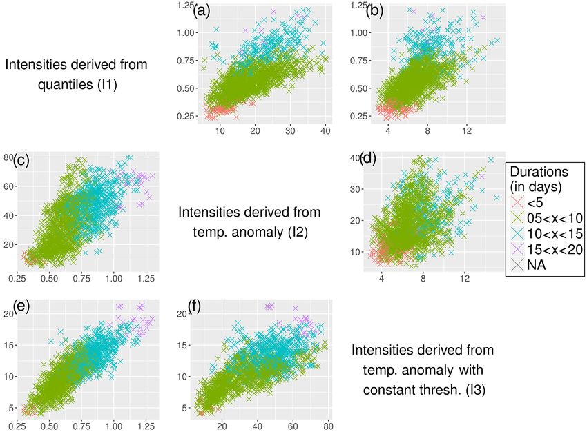
92                                   C. Lavaysse et al.: Towards a monitoring system of temperature extremes in Europe

the human body and its thermal environment. For warm con-        station data with reanalysis data. This LisFlood product will
ditions, indices usually consist of combinations of dry-bulb     be eventually used in the operational system for the moni-
temperature and different measures for humidity or wind          toring of extreme-temperature waves. To validate the results,
speed – such as the humidex (Smoyer-Tomic et al., 2003),         a comparison with two other sets of data is performed: the
the net effective temperature (Li and Chan, 2000), the wet-      ERA-Interim reanalysis (ERAI, Dee et al., 2011) and the
bulb globe temperature (Budd, 2009), the heat index (Stead-      EOBS/ECAD dataset Version 14 (Haylock et al., 2008; van
man, 1979) or the apparent temperature (Steadman, 1984).         den Besselaar et al., 2011), both regridded to the same one
More generally, efforts have been made to harmonize the          square degree resolution. Note that, according to ECMWF,
large number of indices developed. For example, the Univer-      ERAI datasets are released with a delay of 2 months for qual-
sal Thermal Climate Index (UTCI, www.utci.org) has been          ity assurance; as a consequence, this dataset cannot be used
proposed to assess heat and cold waves. The main incon-          for operational monitoring purposes. The same problem oc-
venience of most of these indices is technical – i.e. the hu-    curs for the EOBS datasets.
midity when the daily maximum or daily minimum tem-                 The definition of Tmax and Tmin in the three datasets can
perature (hereafter Tmax and Tmin ) occur is not necessarily     differ from the definition of WMO (van den Basselaar et al.,
known. In addition, the simulated values of wind speed and       2012). In LisFlood, the Tmin assigned to the day d is defined
humidity provided by numerical weather models are gener-         as the minimum temperature value that occurred from 18:00
ally less accurate than the 2 m temperature in the reanalysis    local time (LT) of the day before (d − 1) to 06:00 LT of the
and observational datasets. The WMO Expert Team on Cli-          day d. For EOBS, Tmin is defined as the 24 h daily minimum.
mate Change Detection and Indices (ETCCDI) proposed the          Similarly, Tmax of the day d is the maximum temperature
Warm Spell Duration Index (WSDI) as standard measure-            recorded from 06:00 to 18:00 LT of the day d for LisFlood
ment of heat and cold waves, which is calculated using a         data and the 24 h daily maximum for EOBS. In ERAI, Tmin
percentile-based threshold. Russo et al. (2015) proposed a       (Tmax ) of day d is the lowest (highest) value of tempera-
version of this method that provides the amplitude (or inten-    tures recorded at 00:00, 06:00, 12:00 or 18:00 LT of day d.
sity) of a heat wave based on the maximum temperature and        The starting years of the period covered by the datasets are
the interquartile range of yearly maximum temperatures of        also different (1950 for EOBS, 1979 for ERAI and 1990 for
the past period. This method is powerful to compare the heat     LisFlood). In order to be consistent and in view of the fu-
waves at climatological scale over the world and their trends    ture use for the re-forecast period of the ECMWF ENS fore-
with a local standardization. Nevertheless, this method is not   cast model, the period from 1995 to 2015 (21 years) is used
suitable for monitoring heat waves because it focuses on the     for all the datasets. Note that most of the results obtained
most extreme events (the thresholds are defined according        in this study have been compared to a longer period (start-
to the yearly maxima), and it does not take into account the     ing from 1990) providing very similar results. According to
strong human impact of Tmin (WMO, 2015).                         WMO (2009), the recommended durations of climate sam-
   In this study we propose an operational system to monitor     ples depend on the purpose of the study: climate evolution,
heat and cold waves based on an adapted index inspired by        detection of extremes, climatological reference, climatologi-
the previous studies. In Sect. 2, data and methods are pre-      cal evolution of extremes, etc. However, there is no clear con-
sented and the uncertainties related to the observations are     sensus about a specific duration. As the purpose of this mon-
assessed. Then, the climatology in terms of occurrence, in-      itoring system is the detection of relatively intense events
tensity and duration of the waves are presented in Sect. 3.      according to a reference period, we consider that 20 years
This represents the baseline of the monitoring system that       is sufficient to provide a robust climatology. This baseline
will become operational and embedded in the EDO system.          duration is used in plenty of studies/datasets (Kharin et al.,
Finally, concluding remarks are provided in Sect. 4.             2013; Vautard et al., 2013; Monhart et al., 2016). It is also
                                                                 worth noting that ECMWF runs an extended ensemble model
                                                                 with hindcast (or re-forecast) to create a climatological base-
2     Data and tools                                             line to correct the model bias, build a climatology and detect
                                                                 the strongest anomalies (Vitart, 2004). These hindcasts are
2.1    Datasets                                                  also performed using 21 years, highlighting the usefulness of
                                                                 this length of climatological reference. Moreover, the use of
In this study we use daily Tmax and Tmin from three differ-      a longer period of sampling to estimate the climatology and
ent datasets. The first one is based on the 2 m temperature      to calculate the return period could underestimate the actual
datasets provided by the European National Weather Ser-          return periods of the events due to the non-stationarity of the
vices, which, in turn, is used as an input for the LisFlood      occurrences and intensities of heat and cold waves in the con-
hydrological model (De Roo et al., 2000). The observations       text of climate change (Gonzales-Hidalgo et al., 2016). Ac-
are gridded onto a regular lat/long grid of one square degree.   cording to the WMO guideline (WMO, 2009) and the men-
The use of gridded observation data makes it possible (i) to     tioned previous studies, but also (i) due to the availability of
focus on large-scale heat/cold waves and (ii) to compare the     the datasets and (ii) to be consistent with the forecasts that

Nat. Hazards Earth Syst. Sci., 18, 91–104, 2018                            www.nat-hazards-earth-syst-sci.net/18/91/2018/
C. Lavaysse et al.: Towards a monitoring system of temperature extremes in Europe                                                     93

will be implemented in the same system in the future, we
decided to use the 21-year climatology to detect and charac-
terize the intensities of heat and cold waves.

2.2   Metric of extreme-temperature anomalies

Following the WMO definition, there are many different
ways to measure a heat wave (Perkins et al., 2013). The ob-
jective of this study is not to create a new index, but to pro-
vide an operational system based on an adapted method pro-
posed in the literature. This system is inspired by the studies
of Russo et al. (2014) and WMO (2015). First, daily Tmin            Figure 1. Schema of the detection method and the calculation of
and Tmax are transformed into quantiles based on the clima-         the intensities of heat waves, based on temperature anomalies of a
                                                                    calendar day threshold: Q90 (Tmax ) and Q90 (Tmin ) (I2 calculation),
tological (21 years) calendar percentiles of each variable. To
                                                                    or based on the constant climatological threshold defined by the
highlight the events with the most potential human impact,          median of the daily quantiles: Med (Q90 (Tmax )) and Med (Q90
the year is split into two periods: the extended summer pe-         (Tmin )) (I3 calculation).
riod, when heat waves usually have stronger impacts (the
six hottest months over Europe, from April to September),
and the extended winter period to focus on the cold waves           recommendation of WMO (2015) for health impacts, we de-
(from October to March). Note that also during the sum-             fine a heat (cold) wave as an event of at least 3 consecutive
mer (winter) period, cold (heat) waves may occur but they           hot (cold) days (i.e. when simultaneously Tmin and Tmax ex-
are not considered here. The independent calculation of the         ceed the quantile thresholds). A pool is also introduced when
daily quantiles of observed Tmin and Tmax is done by apply-         two events are separated by 1 day. Note that periods in be-
ing a leave-one-out method to avoid inhomogeneities (Zhang          tween two waves are not taken into account in the wave dura-
et al., 2005). The year studied is removed from the climatol-       tion and in the wave intensity. Figure 1 illustrates the method
ogy. The data without this year is used to derive the observed      used to detect heat waves in this study.
cumulative distribution function (CDF). To remove artefacts            The European mean distribution of these cases is presented
due to the relative small sampling (21 years), a window of          in Tables 1 and 2 using the LisFlood dataset, but the results
11 days centred on the day studied is exploited. The daily          are very similar with the two other datasets (not shown). In
temperatures are transformed into quantiles by this procedure       the first column of both Tables 1 and 2 the number of hot
to create two daily temperature quantiles from 1995 to 2015,        (cold) days (above or under the quantile thresholds) are in-
derived from the CDF of Tmin and Tmax independently.                dicated. Theoretically these values should be constant and
   The main difference from previous studies is the use of          equal to 10 % of the total length of the samplings. Neverthe-
both Tmax and Tmin , rather than Tmax only or the daily mean        less, due to undefined values and values equal to the thresh-
temperature. Thus, a hot day is defined when simultaneously         olds, there are some differences. These tables demonstrate
the daily quantiles of Tmax and Tmin are above quantile 0.9         also the impact of using the intersection of Tmin and Tmax
during the extended summer (from April to September). The           above (below) the thresholds. With respect to heat waves (Ta-
same definition is applied for cold days when the two quan-         ble 1), for example, in about 150 out of 376 days (i.e. 40 %)
tiles are lower than quantile 0.1 from October to March. The        the Tmin above the thresholds occurred simultaneously (i.e.
occurrences are strongly influenced by these thresholds. As         the same day) with Tmax above the threshold (Table 1, first
this study aims at quantifying the intensity of waves regard-       column). Also, there is a significantly higher persistence of
ing the climatology and at assessing with robust scores the         Tmax than Tmin . For instance, using Tmax only, 70 % of the
forecast of these events, it is not possible to focus only on the   hot days (269 out of the 382) are detected as being part of a
most extreme cases. So these thresholds (quantiles 0.9 and          heat wave, whereas using Tmin only, the ratio is about 60 %
0.1) are chosen as a compromise between the need to have            (i.e. 226 out of 376). Using both Tmax and Tmin , on average
a minimum number of events and the definition of extremes.          81.3 days (54 % of the hot days) are detected as being part of
They are also used in a large number of other studies (WMO,         a heat wave (Table 1, second column). Finally, the mean oc-
2015, Hirschi et al., 2011). Note that in order to discuss the      currences of heat waves are indicated in the last column. The
sensitivity of using the intersection of Tmin and Tmax rather       use of the two temperatures tends to reduce drastically the
than one temperature value per day, the same methodology            number of events (from 44 or 51 to 16.9 on average during
has also been applied using separately Tmin and Tmax to de-         the period) but also their durations (5.11 or 5.3 days to 4.8).
termine hot and cold days.                                          The continental regions appear less affected by this reduc-
   Heat and cold waves are associated with a persistence of         tion than coastal regions (not shown). Analogously, Table 2
hot or cold days. Based on the literature (Gasparrini and           shows the same data for cold waves.
Armstrong, 2011; Kuglitsch et al., 2010), as well as on the

www.nat-hazards-earth-syst-sci.net/18/91/2018/                                  Nat. Hazards Earth Syst. Sci., 18, 91–104, 2018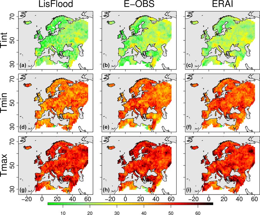
94 C. Lavaysse et al.: Towards a monitoring system of temperature extremes in Europe
Table 1. Spatial mean (and standard deviation in parentheses) of to- quantifying intensities with respect to the seasonal cycle and
tal number of days detected as hot days (larger than quantile 0.9, reflects an anomaly but not necessarily extreme values of ab-
first column), over the entire period (21 years) of analysis, spatial solute temperatures. This calculation is motivated, for exam-
mean of total days detected during heat waves (HW, with persis- ple, by agricultural applications, where the crop yields can be
tence longer than 3 days, second column) during the same period sensitive to strong anomalies during the transitional seasons
and spatial mean of total number of HW during the 21 years (third
(Porter and Semenov, 2005). The last method is also based
column) using only Tmin (first row), only Tmax (second row) and
the intersection of the two variables (Tint , third row).
on temperature anomalies but uses a constant threshold:
h i
N
T − T
Tni,w − Tnmed Q
Hot days Days in HW Number of HW
X i,wx x med (QTx ) ( Tn )
I3(n) = β +
(3)
2 × σTx 2 × σTn
i=1
Tmin 376 (17.9) 226 (31.8) 44.2 (5.1)
Tmax 382 (10.7) 269 (31.0) 51 (4.9)
β = 1 for heat waves
Tint 150 (36.3) 81.3 (33.9) 16.9 (6.1) β = −1 for cold waves.
Here Txmed(QT ) and Tnmed(QT ) represent the constant temper-
Table 2. Same as Table 1 for the cold days and cold waves (CW). x n
ature of the median of all calendar daily quantiles of 0.9
(heat waves) and 0.1 (cold waves) of Tmax and Tmin . The
Cold days Days in CW Number of CW
σTx and σTn represent the climatological yearly variance of
Tmin 380 (20.8) 272 (30.5) 50 (5.3) Tmax and Tmin . This method is intended to increase the in-
Tmax 380 (14.8) 282 (27.4) 50.3 (4.3) tensities of heat or cold waves that occur close to the maxi-
Tint 196 (48.2) 128 (42.7) 25.2 (7.6) mum or minimum of the seasonal cycle. Based on this calcu-
lation, the strongest intensities are generally associated with
the warmest or coldest absolute temperatures. The division
Once a wave is detected, two main characteristics are de- by the variance of the seasonal cycle is justified in order to
rived: the duration (in days) and the intensity. To take into reduce the intensity of the waves that occur over a region with
account different characteristics and to assess the sensitiv- strong seasonal cycle, where the variability of temperature is
ity of the methods, the latter is calculated by three different well known to be significant. The latter method is conceptu-
methods. The first one is based on the sum of the quantiles ally close to the one proposed by Russo et al. (2015) and, due
above (or under) the threshold during the detected wave: to its sensitivity to the absolute temperatures, might be more
h i suitable to assess the potential impacts on human health. Fig-
XN Qtxi,w − Thres + Qtni,w − Thres ure 1 illustrates the heat wave detection and the calculation
I1(n) = β (1) of the two last methodologies. The different intensities pro-
i=1
2 vided by these three methods, which use the same detection
β = 1 for heat waves method, are discussed in the results section.
β = −1 for cold waves.
Here I1 is the intensity of the wave having a duration equal 3 Results
to N days (except the pool days), Qtn and Qtx are the daily
3.1 Comparison of the datasets
quantile of Tmin and Tmax at grid point w and Thres, the quan-
tile thresholds (i.e. 0.9 and 0.1 for heat and cold days respec- In order to compare the observations and quantify the uncer-
tively). The purpose of dividing this intensity by 2 is to cre- tainties of the results, different datasets, provided by obser-
ate an intensity comparable to the intensities calculated with vations and reanalysis, are used. First, the temporal correla-
Tmin and Tmax only. The second method is similar to the first tions between different pairs of the daily quantiles are shown
but the quantile differences are replaced by the temperature in Fig. 2. We notice that the correlation of the quantiles
anomalies with respect to the climatological daily thresholds. of Tmin and Tmax from ERAI, EOBS and LisFlood datasets
This method is defined as follows: are quite in agreement (the spatial mean correlation is about
N
0.89). Note that due to the fact that the quantiles are used,
X Txi,w − QTx + Tni,w − QTn ]
I2(n) = β (2) the seasonal cycle is removed, showing the quality of this
i=1
2 agreement. The scores are generally better for Tmax than
Tmin . This can be explained by the larger spatial homogene-
β = 1 for heat waves
β = −1 for cold waves. ity of Tmax than Tmin and the differences in the Tmin defini-
tion amongst National Weather Services. Indeed, over cer-
Here QTx and QTn represent the calendar daily thresholds of tain countries, Tmin is measured during night time between
Tmin and Tmax , i.e. the temperatures for the quantiles 0.9 (0.1) 18:00 and 06:00 LT the following day, elsewhere from 00:00
for the heat (cold respectively) waves. This method allows to 24:00 LT or from 06:00 LT on day d to 06:00 LT on day
Nat. Hazards Earth Syst. Sci., 18, 91–104, 2018 www.nat-hazards-earth-syst-sci.net/18/91/2018/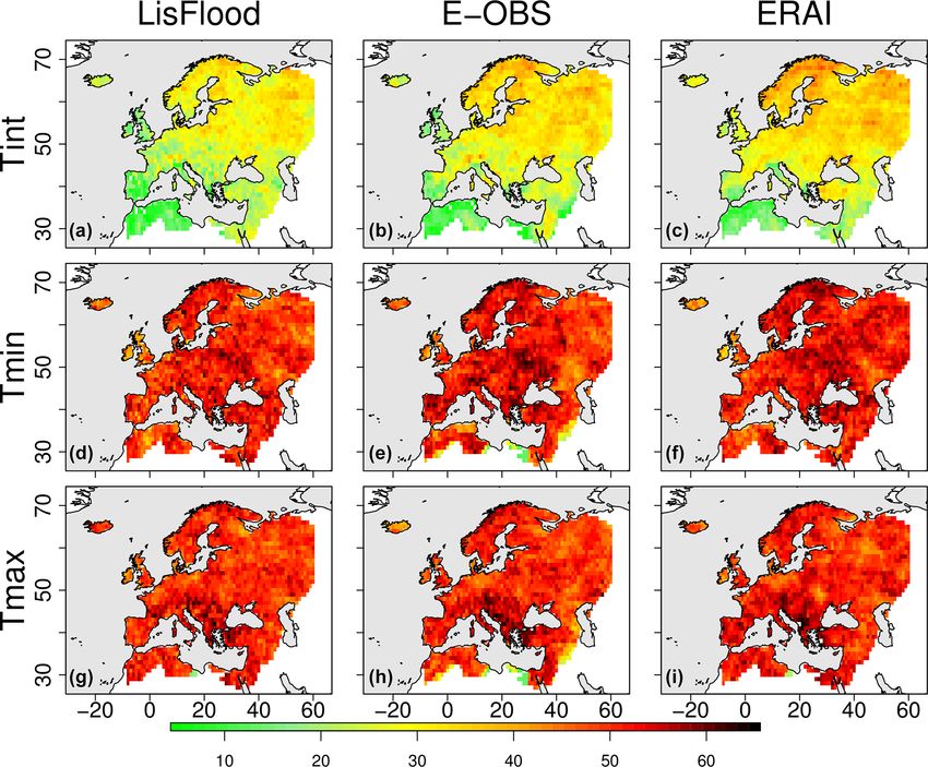
C. Lavaysse et al.: Towards a monitoring system of temperature extremes in Europe                                                       95

Figure 2. Temporal correlation of the temperature quantiles of Tmin (a), and Tmax (b) provided by ERAI, EOBS and LisFlood datasets from
1995 to 2015. The datasets compared are indicated on the top of each column.

Figure 3. Mean absolute error of temperature (in K) between the three datasets, calculated from 1995 to 2015 for Tmin (a) and Tmax (b). The
datasets compared are indicated on the top of each column.

d + 1, which can result in a delay of 1 day. In the EOBS data           relatively low (< 1.5◦ ) except at the borders of the domain,
description, and in van den Besselaar et al. (2011), this point         confirming the good agreement especially between EOBS
and the uncertainties associated are deeply analysed. Due to            and ERAI. Note that the LisFlood dataset is slightly less
the coarser resolution and the use of only four recorded val-           correlated to the others over Scandinavia, Germany and the
ues per day to calculate Tmin and Tmax , ERAI is associated             northeasternmost part of the domain – probably due to the
with a hot bias of Tmin and a cold bias of Tmax in relation to          definition of Tmin and Tmax for each country, delay in the GTS
both LisFlood and EOBS datasets (not shown). The yearly                 communications and the density of the stations (the E-OBS
mean absolute error of Tmin and Tmax (MAE, Fig. 3, very                 network over Germany and Scandinavia is quite dense).
close to the root mean square difference) remains, however,

www.nat-hazards-earth-syst-sci.net/18/91/2018/                                     Nat. Hazards Earth Syst. Sci., 18, 91–104, 2018
96                                     C. Lavaysse et al.: Towards a monitoring system of temperature extremes in Europe

Figure 4. Number of occurrences of heat waves in Europe from 1995 to 2015 using the intersection of both Tmin and Tmax (Tint, a–c), only
Tmin (d–f), and only Tmax (g–i) with LisFlood (a, d, g), E-OBS (b, e, h) and ERAI (c, f, i) datasets.

3.2     Climatology                                                   Doblas-Reyes et al., 2002). Several recent studies (Tomczyk
                                                                      and Bednorz, 2016; Sousa et al., 2017) have emphasized the
3.2.1    Variability in the occurrence of the waves                   important role of persistent and intense blocking and associ-
                                                                      ated anticyclones in producing heat or cold waves. The ori-
The total occurrences of heat and cold waves during the               gins of the extreme blocking situations are still not well un-
21 years are calculated using the definitions presented in            derstood and could be related to the development of a large-
Sect. 2. This is performed independently for the three                scale Rossby train (Trenberth and Fasullo, 2012). Schubert
datasets to provide information on the robustness of the re-          et al. (2014), who identified western Russia as the leading
sults. As shown in Tables 1 and 2, cold waves are more fre-           mode of surface temperature and precipitation covariability,
quent than heat waves for the three datasets, especially in the       have highlighted the potential feedback of the soil moisture
eastern part of Europe (Figs. 4 and 5, first row). The inde-          in enhancing the intensities of the heat waves over this region
pendent use of Tmin and Tmax to detect, respectively, heat and        (Fisher et al., 2007; Mueller and Seneviratne, 2013; Miralles
cold waves reveals more homogeneous spatial patterns and a            et al., 2014; Whan et al., 2015).
similar rate of occurrence across the three datasets, but about          The main difference between the datasets is the higher oc-
50 to 60 % more than for the intersection of Tmin and Tmax            currence of both heat and cold waves for ERAI than for the
(Figs. 4 and 5, second and third row). The detection of the           other datasets. This could be an effect of the coarser reso-
heat waves using Tmin only generates fewer events. These re-          lution in time and space of the reanalysis data compared to
sults highlight two main characteristics: (1) the lower per-          the ground observations, which tends to smooth the temporal
sistence of Tmin with strong anomalies could partially ex-            evolution of the temperature anomalies and so of the quan-
plain the difference between the occurrence of heat and cold          tiles. Due to that lower temporal variability, the chance to get
waves; (2) the increase of the occurrence in the continental          long-term anomalies is increased when using ERAI as com-
regions is mainly explained by an increase of the simultane-          pared to the other datasets.
ous anomalies in Tmin and Tmax rather than an increase of                The distribution of the wave durations is needed to com-
the two occurrences. These two characteristics may be ex-             plete the picture of the total number of occurrences of all
plained by the synoptical situations during cold waves and            individual waves. Figure 6 displays the spatial variability
the fact that there are more frequent meteorological block-           of the last quartile of the wave durations recorded for each
ing conditions in winter than in summer (Tibaldi et al., 1994;

Nat. Hazards Earth Syst. Sci., 18, 91–104, 2018                                  www.nat-hazards-earth-syst-sci.net/18/91/2018/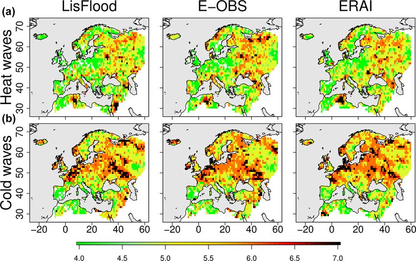
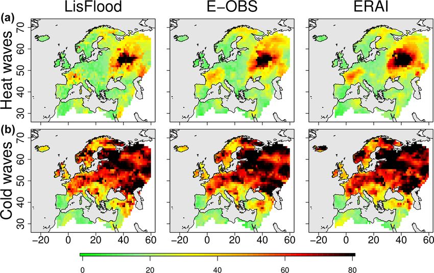
C. Lavaysse et al.: Towards a monitoring system of temperature extremes in Europe                                                      97

Figure 5. Number of occurrences of cold waves in Europe from 1995 to 2015 using the intersection of both Tmin and Tmax (Tint, a–c), only
Tmin (d–f), and only Tmax (g–i) with LisFlood (a, d, g), E-OBS (b, e, h) and ERAI (c, f, i) datasets.

Figure 6. Last quartile of the wave durations (in days) for the heat (a) and cold (b) waves using LisFlood, E-OBS and ERAI datasets.

grid point. It appears that the difference between the du-             waves are the most frequent are not the same as where they
rations of heat and cold waves between the three different             are the most persistent. Finally, it is remarkable to see many
datasets is much lower than the difference of occurrence dis-          of the longest durations of the cold waves along the coasts of
cussed previously (Figs. 4 and 5). It is also interesting to           the North Sea and the Baltic Sea. Indeed, the climate along
note that, especially for cold waves, the regions where the            the coasts is generally more variable than in the continental

www.nat-hazards-earth-syst-sci.net/18/91/2018/                                     Nat. Hazards Earth Syst. Sci., 18, 91–104, 2018
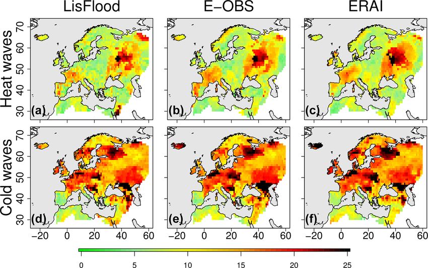
98 C. Lavaysse et al.: Towards a monitoring system of temperature extremes in Europe
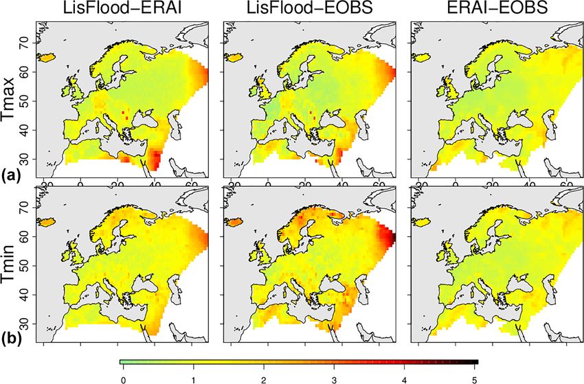
Figure 7. Matrix of scatter plots of the three intensity calculations related to quantiles, temperature anomalies and temperatures anomalies
with constant thresholds (I1, I2 and I3 respectively) during heat (a, b, d) and cold (c, e, f) waves using LisFlood. The colours indicate the
duration (in days) of each wave.
regions, and so the waves are expected to be shorter. Ac- 3.2.2 Intensity of the heat and cold waves
cording to the same calculations using only Tmin or Tmax
(not shown), the spatial heterogeneity of the cold wave du- The climatology of the intensities is important in order to
rations is much larger when Tmax is used than when Tmin provide a baseline and to calibrate the wave monitored but
is used and we observe a strong increase of the wave du- the values of these intensities are very sensitive to the meth-
rations with Tmax over northern Germany, Denmark, north- ods applied. The three methods, I1, I2 and I3 (using the quan-
ern Poland, the Baltic Sea and southern Scandinavia. This tiles, the temperature anomalies and the constant threshold
highlights the persistence of negative anomalies of Tmax over of temperature, see Sect. 2.2), are compared during heat and
these regions, which could increase the chance to get longer cold waves in Fig. 7. The distributions of each scatter plot in-
durations with the intersection method and could explain the dicate the relationships by pairs in between the three methods
results in Fig. 6. In other words, the Baltic Sea stabilizes for all the events, and the colours indicate the correspond-
the temperature variability and therefore generates a signal ing durations of the events. Note that Fig. 7 refers to Lis-
with lower high-frequency modulations. When an anomaly Flood, but the same results are obtained for the other datasets.
occurs, it has a greater chance of lasting longer and so po- These panels show the strong dependence of the intensities
tentially induce longer heat/cold waves. This is due to our derived from the quantiles and the durations (colour distribu-
detection method of heat and cold waves that is based on tion more vertically distributed in Fig. 7b and horizontally in
the quantiles and not on absolute temperatures. The latter are Fig. 7c and e). This is especially true for the cold waves (cor-
generally less variable and less extreme values are detected relations in between duration and I1 larger than 0.95). These
along the coasts. In addition, the wavelet analysis (Torence high correlations highlight the redundancy in the information
and Compo, 1998) of temperature in winter and summer was with the wave durations. Moreover, I1 is also climatologi-
also calculated to analyse the frequency variabilities of the cally bounded by the values recorded during the past period.
signal. This showed that the regions with low modulations For these reasons the use of the quantiles appears not suit-
(eastern Europe in summer or northern Russia and the north able to assess the heat and cold wave intensities. The meth-
of Poland in winter) are also the regions with high frequency ods derived from the temperature anomaly (I2) and the con-
of occurrence or with longer durations (not shown). stant threshold (I3) are therefore chosen. Indeed, the correla-
tions between the wave durations and I2 and with I3 are much
lower and not significant (on average 0.72 and 0.59), show-
ing the potential additional information provided by I2 and
Nat. Hazards Earth Syst. Sci., 18, 91–104, 2018 www.nat-hazards-earth-syst-sci.net/18/91/2018/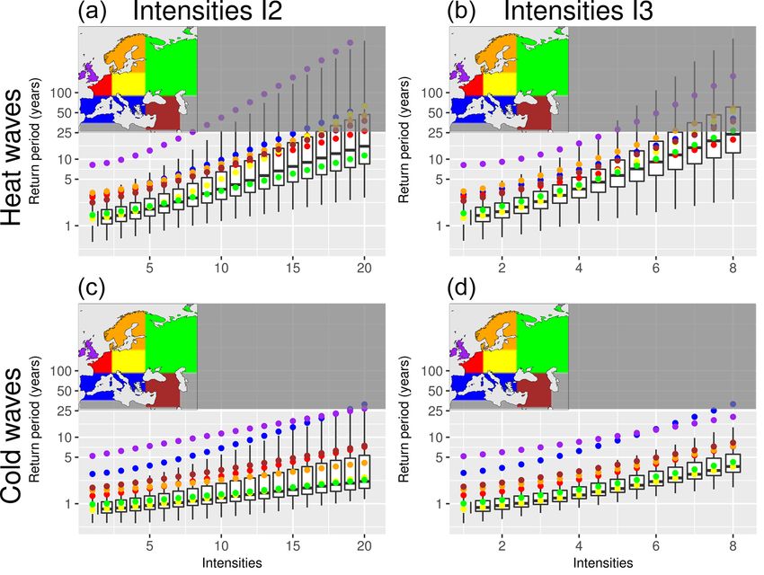
C. Lavaysse et al.: Towards a monitoring system of temperature extremes in Europe                                                      99

Figure 8. Histograms of heat (a) and cold (b) wave intensities defined as temperature anomalies (I2) for the three datasets. Note that the
frequency axes are on a log scale.

I3. Moreover, these values are not bounded by the historical           that the relatively short period of study (21 years) could gen-
values and so they will be able to better distinguish the most         erate some artefacts over regions that recorded extraordinary
severe cases. According to the scatter plots in Fig. 7d (for the       events (e.g. Russia).
heat waves) and Fig. 7f (for the cold waves), these methods               To assess meteorological uncertainties, Fig. 10 displays
appear quite independent at the European scale. Neverthe-              the same distributions but for intensities calculated using
less, the analysis of the correlations at the grip point level re-     constant thresholds (I3). Although the scales are different,
veals a large spatial variability (not shown). For instance, the       the spatial distribution of I2 and I3 for the strongest heat
correlations of I2 and I3 go up to 0.95 over France and west-          waves is quite similar. The patterns are strongly influenced
ern Russia, explained by heat (cold) waves that occurred dur-          by the two heat waves in 2003 and 2010. In contrast, the
ing the warmest (coldest) months, and go down to 0.5 over              distribution of the strongest cold waves changes drastically.
central and northern Europe.                                           While the intensities over Russia are reduced, we note a rel-
   Except for the strongest events, there is an overall good           ative increase of the intensities over western Europe, espe-
agreement of the datasets in terms of the probability distri-          cially in north Germany, the Netherlands, and in central Eu-
bution functions of the intensities of heat and cold waves.            rope. As discussed previously, this could be explained by
Figure 8 displays the distribution of intensities defined by           events that occurred during the transitional months (intense
the method of the temperature anomalies (I2) and shows no              I2 but not I3) or close to the maximum (or minimum) sea-
significant differences for intensities lower than 60. This fig-       sonal temperature (intense I3). The spatial distribution is also
ure also confirms our finding of the higher occurrence of              influenced by the normalization according to the amplitude
cold waves than heat waves especially with intensities larger          of the seasonal cycle, which is larger in continental regions
than 25. In the tails of the distribution (especially for the heat     (not shown). Even if the results display significant differ-
waves larger than 90), the differences are associated with a           ences according to the methods and the regions, it is impor-
very low number of cases. The spatial variability of these             tant to note that the three datasets are still in good agreement.
I2-based intensities in the last 21 years was assessed by the
strongest cold and heat waves recorded over each grid point            3.3   Return periods
(Fig. 9). The two strongest heat waves that occurred in Eu-
rope can be clearly identified, namely the one that occurred           As the purpose of this study is to provide a methodology that
in Russia in 2010 and the one in France in 2003. For these             is usable for a monitoring system that must be robust and
two events, the intensities are slightly stronger and longer           understandable for users and decision makers, the informa-
using ERAI (not shown). For the cold waves, the intensities            tion should also be provided in terms of return periods. This
are stronger than the heat waves. The most intense events oc-          product will quantify, at the monthly timescale, the inten-
curred over the continental regions (central Europe and the            sity of the cold or heat waves that have occurred. To build
south of Russia). The three datasets are in good agreement             this indicator, all the days defined as cold or heat waves are
for the intensities and the spatial variabilities. It is interesting   summed for different accumulation periods (from monthly to
to highlight that these intensities are not well correlated to the     seasonally, see Table 3). Monthly values characterize either
occurrence – i.e. a region with more cases does not necessar-          one specific event as defined previously or several consecu-
ily record the most extreme events (Figs. 4 and 5). We note            tive cases. As indicated by WMO (2015), intense or repetitive

www.nat-hazards-earth-syst-sci.net/18/91/2018/                                     Nat. Hazards Earth Syst. Sci., 18, 91–104, 2018
100                                      C. Lavaysse et al.: Towards a monitoring system of temperature extremes in Europe

Figure 9. Spatial distribution of the strongest heat (a) and cold (b) waves intensities, defined as temperature anomalies (I2), using LisFlood,
E-OBS and ERAI datasets.

Figure 10. Same as Fig. 9 using the intensity based on the constant threshold (I3) for heat (a–c) and cold (d–f) waves, and based on
LisFlood (a, d), E-OBS (b, e) and ERAI (c, f).

extreme waves may have strong impacts on human health and                 According to the Pearson goodness-of-fit statistic, and the
so should be assessed. Once these monthly values are calcu-               deviance statistic on the entire distribution, the gamma dis-
lated for each grid point, the return period is estimated. Prob-          tribution is the most suitable (not shown). By using this theo-
lems when dealing with extremes are linked to erroneous                   retical distribution, the return periods can be extrapolated be-
values and the sampling. To partially address these issues,               yond the 21-year period. Once the parameters of the gamma
we have compared different datasets, and different theoreti-              distribution are estimated for monthly, bimonthly and sea-
cal distributions have been fitted and tested. This is done at            sonal timescales (see Table 3), return periods are calculated
both grid-point and regional level. Other distributions have              for both the cold and heat waves. According to significance
been applied in the literature – such as the gamma (Meehl                 tests employed to guarantee the robustness of the distribu-
et al., 2000) or the Weibull distribution (Cueto et al., 2010).           tion, uncertainties exist for return periods larger than the du-

Nat. Hazards Earth Syst. Sci., 18, 91–104, 2018                                      www.nat-hazards-earth-syst-sci.net/18/91/2018/
C. Lavaysse et al.: Towards a monitoring system of temperature extremes in Europe                                                          101

Table 3. Accumulation periods used to calculate the return period of wave intensities. The type of waves (cold or heat) is indicated in the
second row and the accumulation period of the sum of intensities is indicated in the last row (1 for 1-month accumulation period, 2 for
2-month accumulation period and S for Season, i.e. 6-month accumulation period).

               Months        Jan     Feb       Mar     Apr     May      Jun      Jul    Aug        Sep     Oct     Nov      Dec
               Type         Cold    Cold      Cold     Heat    Heat    Heat    Heat     Heat      Heat    Cold    Cold     Cold
               Duration      1, 2    1, 2    1, 2, S      1     1, 2    1, 2    1, 2     1, 2   1, 2, S      1     1, 2     1, 2

Figure 11. Return periods of monthly intensities of heat (a, b) and cold (c, d) waves for two intensities (I2, a, c, and I3, b, d). Boxes assess
the spatial variability for the grid points. Coloured dots indicate the return period calculated over the regions defined in the small panels.

ration of the observed sampling. For these reasons, return pe-            of the boxes), and lower return periods associated with the
riods longer than 25 years are reported with grey shadows                 larger wave intensities (not shown).
and, in addition, the x axis in Fig. 11 is limited in order to               The spatial variabilities are then analysed in more detail
have at least 50 % of grid points not exceeding a 25-year re-             with a regional classification. This classification is a sim-
turn period. Under these conditions, all the events that have             plification of the one shown in the EEA report (2016) that
return periods larger than the duration of the sampling will              takes into account the climatology of the regions (Continen-
not be distinguished and all of them will be considered as the            tal, Mediterranean, Oceanic, Scandinavian, small panels in
“most dangerous”. The return period results were produced                 Fig. 11). Over these regions, the return periods are assessed
using the LisFlood dataset, which has been validated in the               and compared (coloured dots in Fig. 11). Even if the results
previous section, but similar results were obtained with the              for the two intensities (left and right panels) cannot be com-
two other datasets.                                                       pared directly, it is interesting to compare the ranking of the
   The boxplots (Fig. 11) show the relationships between in-              regions according to the return periods. For heat waves, the
tensities and return periods over each grid point in Europe.              British Isles stand out by using the two intensities. The few
According to the size of the interquartiles, a large spatial vari-        intense heat waves recorded generate return periods in the
ability emerges over the domain. For instance, heat waves                 outliers of the box distribution in Europe. In contrast, the
with intensities of 20 (8) using I2 (I3) have interquartiles of           Russian region records the lowest return periods for similar
return period that span from 7 to 50 years (15 to 90 years re-            intensities using I2, showing the large hazard of these heat
spectively). The use of other datasets provides similar results.          waves in this region. Nevertheless, the use of the I3 calcula-
Nevertheless, ERAI has less spatial variability (lower spread             tion (more sensitive to waves that occurred during the heart
                                                                          of the season) shows a different distribution, with more cases

www.nat-hazards-earth-syst-sci.net/18/91/2018/                                         Nat. Hazards Earth Syst. Sci., 18, 91–104, 2018
102 C. Lavaysse et al.: Towards a monitoring system of temperature extremes in Europe
4 Discussion
The purpose of this study was to develop a system to monitor
potential high-impact climate extreme events. Defining the
intensity of an extreme event is important since it provides
the hazard component to be related to human or economic
impacts. Many studies have already dealt with this issue, but
no consensus has been reached so far for heat and cold waves.
Large local differences usually prevent the use of a single
definition for impact-oriented global studies. One option is to
apply a constant threshold such as 35 or 40◦ for heat waves
and −10 or −20◦ for cold waves across an entire continent,
as these definitions are understandable and easy to communi-
cate. Nevertheless, such a choice can be questionable. For ex-
ample, the heat wave in France in 2003 was associated with
absolute temperatures close to 40◦ ; which are relatively close
to the climatology for southern Spain. The impacts, therefore
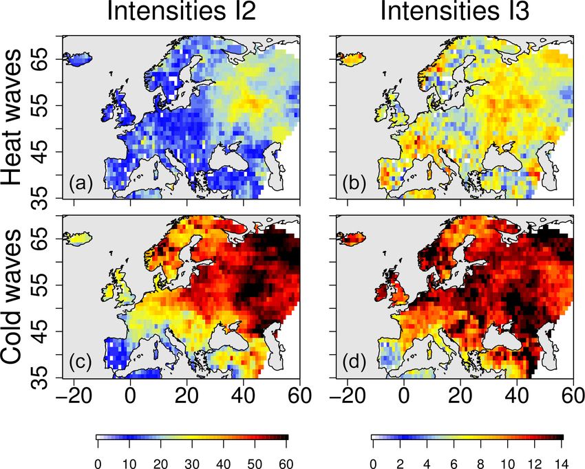
Figure 12. Intensity of the heat (a, b) and cold (c, d) waves defined are not just temperature dependent, but they vary according
with the temperature anomalies (I2, a, c), or with constant thresh- to the geographical location (and thus the local climate), the
olds (I3, b, d) with a 10-year return period using LisFlood dataset. societal exposure and vulnerability. For all these reasons, it is
difficult to identify the most robust indicator. The ones cho-
sen in this study are based on the rarity of the events. The
over central Europe for return periods lower than 5 years (in implicit assumption made is that rarity is associated with a
yellow) and the northwest European region (red) for the most lack of specific adaptation and thus with higher risk.
intense heat waves. For the cold waves, the British Isles and
the Mediterranean regions are the least affected in the two in-
tensity calculations, whereas the continental parts of Europe 5 Summary and conclusions
(Russia and central Europe) are associated with more regular
intense cold waves. In this study, we assessed the feasibility of monitoring heat
In Fig. 12, both I2 and I3 intensities of the heat and cold and cold waves by using a method based on the persis-
waves with a return period of 10 years are plotted. As these tence of the exceedance of quantiles of daily minimum and
values depend on the observed waves in the analysed period, maximum temperatures at grid point level. In the first step,
a hot spot over western Russia appears (Fig. 12a, c). In that three methods to detect and quantify the intensities of heat
region in the last 21 years, waves were more frequent (Figs. 4 and cold waves were assessed. The use of Tmin , Tmax and
and 5) and more intense (Fig. 9). The results with I3 show of both values was investigated. This demonstrated how the
different behaviours (Fig. 12b, d). This is due to the different combined use of the two daily temperatures reduces the fre-
location of the most intense waves (Fig. 10). The potential quency of the extremes. To make the analysis more robust,
impacts of these heat and cold waves will be calculated as three datasets were compared, two derived from station data
a function of the absolute intensities and the return periods. (LisFlood and EOBS) and one from reanalysis data (ERAI).
However, we can expect that identical wave intensities over The two observational datasets showed only minor differ-
two different regions, and therefore with two different return ences in heat and cold waves occurrences and intensities.
periods, may have different impacts. For example, the abso- This is probably due to the good agreement in representing
lute value of the heat wave intensity recorded in August 2003 both Tmin and Tmax . Using ERAI some differences appeared,
over France using I3 does not give extreme values with re- mainly due to the coarser resolution of the original grid and
spect to the intensities recorded in continental regions. Nev- the use of only four values per day to define Tmin and Tmax .
ertheless, the equivalent return value over France is larger In this case, the persistence and the spatial correlation in-
than 50 years (not shown), in agreement with Barriopedro et creased, generating less spatial distinction and more intense
al. (2011) and Trigo et al. (2005), which suggests the poten- waves with respect to the other two datasets. However, the
tial strong associated risk. main results are in overall agreement for all three datasets
Given the 21-year period used in this study, the return pe- and show a larger hazard for heat and cold waves in the con-
riod can identify the most extreme situations. The same in- tinental part of Europe. Return periods were also estimated,
formation will also be available for the 2-month and seasonal and this information will be used operationally in the EDO
timescales (not shown). system to provide robust and comprehensible products for
decision makers and users.
Nat. Hazards Earth Syst. Sci., 18, 91–104, 2018 www.nat-hazards-earth-syst-sci.net/18/91/2018/C. Lavaysse et al.: Towards a monitoring system of temperature extremes in Europe 103
In perspective, these datasets and results should be com- Gasparrini, A. and Armstrong, B.: The impact of
pared to the ones derived from forecast products in order to heat waves on mortality, Epidemiology, 22, 68-73,
be able to provide a comprehensive and seamless tool for https://doi.org/10.1097/EDE.0b013e3181fdcd99, 2011.
monitoring and forecasting heat and cold waves in Europe. Gonzalez-Hidalgo, J. C., Peña-Angulo, D., Brunetti, M., and
Cortesi, N.: Recent trend in temperature evolution in Spanish
mainland (1951–2010): from warming to hiatus, Int. J. Clima-
tol., 36, 2405–2416, 2016.
Data availability. All the data on detection and intensities of the
Haylock, M. R., Hofstra, N., Klein Tank, A. M. G., Klok,
heat and cold waves in Europe are available on demand or on the
E. J., Jones, P. D., and New, M.: A European daily high-
European Drought Observatory web page (http://edo.jrc.ec.europa.
resolution gridded data set of surface temperature and precipi-
eu/).
tation for 1950–2006, J. Geophys. Res.-Atmos., 113, D20119,
https://doi.org/10.1029/2008JD010201, 2008.
Hirschi, M., Seneviratne, S. I., Alexandrov, V., Boberg, F.,
Competing interests. The authors declare that they have no conflict Boroneant, C., Christensen, O. B., Formayer, H., Orlowsky, B.,
of interest. and Stepanek, P.: Observational evidence for soil-moisture im-
pact on hot extremes in southeastern Europe, Nat. Geosci., 4,
17–21, 2011.
Acknowledgements. The authors would like to thank the two Kharin, V. V., Zwiers, F. W., Zhang, X., and Wehner, M.: Changes in
anonymous reviewers for their helpful comments. temperature and precipitation extremes in the CMIP5 ensemble,
Clim. Change, 119, 345–357, 2013.
Edited by: Vassiliki Kotroni Kovats, R. S. and Kristie, L. E.: Heatwaves and public health in
Reviewed by: two anonymous referees Europe, Eur. J. Public Health, 16, 592–599, 2006.
Kuglitsch, F. G., Toreti, A., Xoplaki, E., Della-Marta, P. M., Zere-
fos, C. S., Türkeş, M., and Luterbacher, J.: Heat wave changes in
the eastern Mediterranean since 1960, Geophys. Res. Lett., 37,
L04802, https://doi.org/10.1029/2009GL041841, 2010.
Li, P. W. and Chan, S. T.: Application of a weather stress index for
References alerting the public to stressful weather in Hong Kong, Meteorol.
Appl., 7, 369–375, 2000.
Barriopedro, D., Fischer, E. M., Luterbacher, J., Trigo, R. M., and Meehl, G. A., Karl, T., Easterling, D. R., Changnon, S., Pielke Jr.,
García-Herrera, R.: The hot summer of 2010: redrawing the tem- R., Changnon, D., Evans, J., Groisman, P., Knutson,T., Kunkel,
perature record map of Europe, Science, 332, 220–224, 2011. K., and Mearns, L. O.: An introduction to trends in extreme
Budd, G. M.: The wet-bulb globe temperature: its history and limi- weather and climate events: observations, socioeconomic im-
tations, J. Sci. Medicine in Sport, 11, 20–32, 2009. pacts, terrestrial ecological impacts, and model projections, B.
Cueto, R. G., Martinez, A. T., and Ostos, E. J.: Heat waves and heat Am. Meteorol. Soc., 81, 413–416, https://doi.org/10.1175/1520-
days in an arid city in the northwest of Mexico: current trends 0477(2000)0812.3.CO;2, 2000.
and in climate change scenarios, Int. J. Biometeorol., 54, 335– Miralles, D. G., Teuling, A. J., van Heerwarden, C. C., and Vilà-
345, 2010. Guerau de Arellano, J.: Mega-heatwave temperatures due to
de’Donato, F. K., Leone, M., Noce, D., Davoli, M., and Mich- combined soil desiccation and atmospheric heat accumulation,
elozzi P.: The Impact of the February 2012 Cold Spell on Nat. Geosci., 7, 345–348, 2014.
Health in Italy Using Surveillance Data, PLoS ONE, 8, e61720, Mueller, B. and Seneviratne, S.: How soils send mes-
https://doi.org/10.1371/journal.pone.0061720, 2013. sages on heat waves, IGBP’s Global Change maga-
Dee, D. P., Uppala, S. M., Simmons, A. J., Berrisford, P., Poli, P., zine, No. 81, available at: http://www.igbp.net/news/
Kobayashi, S., and Bechtold, P.: The ERA-Interim reanalysis: features/features/howsoilssendmessagesonheatwaves.5.
Configuration and performance of the data assimilation system, 30566fc6142425d6c911a33.html, October 2013.
Q. J. Roy., Meteor. Soc., 137, 553–597, 2011. Monhart, S., Spirig, C., Bhend, J., Liniger, M. A., Bogner, K., and
De Roo, A. P. J., Wesseling, C. G., and Van Deursen, W. P. A.: Phys- Schär, C.: Verification of ECMWF monthly forecasts for the use
ically based river basin modelling within a GIS: the LISFLOOD in hydrological predictions, EGU General Assembly Conference
model, Hydrol. Process., 14, 1981–1992, 2000. Abstracts, 18, 14122, 2016.
Doblas-Reyes, F. J., Casado, M. J., and Pastor, M. A.: Sensi- Montero, J. C., Mirón, I. J., Criado-Álvarez, J. J., Linares, C., and
tivity of the Northern Hemisphere blocking frequency to the Díaz, J.: Influence of local factors in the relationship between
detection index, J. Geophys. Res.-Atmospheres, 107, 4009, mortality and heat waves: Castile-La Mancha (1975–2003), Sci.
https://doi.org/10.1029/2000JD000290, 2002. Total Environ., 414, 73–80, 2012.
EEA report: Climate Change, impacts and vulnerability in Europe Perkins, S. E. and L. V. Alexander: On the measurement of heat
in 2016, an indicator-based report, EEA report (1/2017), ISSN waves, J. Climate, 26, 4500–4517, 2013.
1977-8449, 2016. Porter, J. R. and Semenov M. A.: Crop responses to climatic varia-
Fischer, E. M., Seneviratne, S. I., Vidale, P. L., Lüthi, tion, Philos. T. Roy. Soc. B, 360, 2021–2035, 2005.
D., and Schär, C.: Soil-Atmosphere interactions during the Robine, J. M., Cheung, S. L. K., Le Roy, S., Van Oyen, H., Grif-
2003 European summer heat wave, J. Climate, 5081–5099, fiths, C., Michel, J. P., and Herrmann, F. R.: Death toll exceeded
https://doi.org/10.1175/JCLI4288.1, 2007.
www.nat-hazards-earth-syst-sci.net/18/91/2018/ Nat. Hazards Earth Syst. Sci., 18, 91–104, 2018104 C. Lavaysse et al.: Towards a monitoring system of temperature extremes in Europe 70,000 in Europe during the summer of 2003, C. R. Biol., 331, Trenberth, K. E. and Fasullo, J. T.: Climate extremes and 171–178, 2008. climate change: The Russian heat wave and other climate Rocklov, J., Barnett, A. G., and Woodward, A.: On the estimation extremes of 2010, J. Geophys. Res.-Atmos., 117, D17103, of heat-intensity and heat-duration effects in time series models https://doi.org/10.1029/2012JD018020, 2012. of temperature-related mortality in Stockholm, Sweden, Environ. Trigo, R. M., García-Herrera, R., Díaz, J., Trigo, I. F., and Health, 11, 23, https://doi.org/10.1186/1476-069X-11-23, 2012. Valente, M. A.: How exceptional was the early August Rooney, C., McMichael, A. J., Kovats, R. S., and Coleman, M. P. : 2003 heatwave in France?, Geophys. Res. Lett., 32, L10701, Excess mortality in England and Wales, and in Greater London, https://doi.org/10.1029/2005GL022410, 2005. during the 1995 heatwave, J. Epidemiol. Commun. H., 52, 482– Van den Besselaar, E. J. M., Haylock, M. R., Van der 486, 1998. Schrier, G., and Klein Tank, A. M. G.: A European Russo, S., Dosio, A., Graversen, R. G., Sillmann, J., Carrao, H., daily high-resolution observational gridded data set of sea Dunbar, M. B., and Vogt, J. V.: Magnitude of extreme heat waves level pressure, J. Geophys. Res.-Atmos., 116, D11110, in present climate and their projection in a warming world, J. https://doi.org/10.1029/2010JD015468, 2011. Geophys. Res.-Atmos., 119, 12500–12512, 2014. Van den Besselaar, E. J. M., Klein Tank, A. M. G., Van der Russo, S., Sillmann, J., and Fischer, E. M.: Top ten European heat- Schrier, G., and Jones, P. D.: Synoptic messages to extend waves since 1950 and their occurrence in the coming decades, climate data records, J. Geophys. Res.-Atmos., 117, D07101, Environ. Res. Lett., 10, 124003, https://doi.org/10.1088/1748- https://doi.org/10.1029/2011JD016687, 2012. 9326/10/12/124003, 2015. Vautard, R., Gobiet, A., Jacob, D., Belda, M., Colette, A., Déqué, Schubert, S. D., Wang, H., Koster, R. D., Suarez, M. J., and Gro- M., and Halenka, T.: The simulation of European heat waves isman, P. Y.: Northern Eurasian heat waves and droughts, J. Cli- from an ensemble of regional climate models within the EURO- mate, 27, 3169–3207, 2014. CORDEX project, Clim. Dynam., 41, 2555–2575, 2013. Smoyer-Tomic, K. E., Kuhn, R., and Hudson, A.: Heat wave haz- Vitart, F.: Monthly forecasting at ECMWF, Mon. Weather Rev., ards: an overview of heat wave impacts in Canada, Nat. Hazards, 132, 2761–2779, 2004. 28, 465–486, 2003. Whan, K., Zscheischler, J., Orth, R., Shongwe, M., Rahimi, M., Sousa, P. M., Trigo, R. M., Barriopedro, D., Soares, P. Asare, E. O., Seneviratne, S. I.: Impact of soil moisture on ex- M., and Santos, J. A.: European temperature responses to treme maximum temperatures in Europe, Weather Climate Ex- blocking and ridge regional patterns, Clim. Dynam., 1–21, tremes, 9, 57–67, 2015. https://doi.org/10.1007/s00382-017-3620-2, online first, 2017. WMO: Data, Climate, Guidelines on analysis of extremes in a Steadman, R. G.: The assessment of sultriness, Part I: A changing climate in support of informed decisions for adaptation, temperature-humidity index based on human physiology and available at: https://library.wmo.int/opac/index.php?lvl=notice_ clothing science, J. Appl. Meteorol., 18, 861–873, 1979. display&id=138#.WkzgMq0cBGo, 2009. Steadman, R. G.: A universal scale of apparent temperature, J. Clim. WMO: Heatwaves and health: guidance on warn- Appl. Meteorol., 23, 1674–1687, 1984. ing system development, WMO-No. 1142, World Tibaldi, S., Tosi, E., Navarra, A., and Pedulli, L.: Northern and Meteorological Organisation, available at: http: Southern Hemisphere seasonal variability of blocking frequency //www.who.int/entity/globalchange/publications/ and predictability, Mon. Weather Rev., 122, 1971–2003, 1994. Web-release-WHO-WMO-guidance-heatwave-and-health. Tomczyk, A. M. and Bednorz, E.: Heat waves in Central Europe pdf?ua=_1 (last access: 3 January 2017), 2015. and their circulation conditions, Int. J. Climatol., 36, 770–782, Zhang, X., Hegerl, G., Zwiers, F. W., and Kenyon, J.: Avoiding 2016. inhomogeneity in percentile-based indices of temperature ex- Torrence, C. and Compo, G. P.: A practical guide to wavelet analy- tremes, J. Climate, 18, 1641–1651, 2005. sis, B. Am. Meteorol. Soc., 79, 61–78, 1998. Nat. Hazards Earth Syst. Sci., 18, 91–104, 2018 www.nat-hazards-earth-syst-sci.net/18/91/2018/
You can also read